WorldModels:Tutorial:13-ModernWorldModels
lastmod 2026-11-18created 2026-11-172 edits
The Modern World Model Landscape is chapter 13 of the World Model tutorial. Using the reconstruction-based World Models built through chapter 12 (VAE, MDN-RNN, RSSM, Dreamer) as a reference point, it places the post-2019 families on a single map: MuZero, TD-MPC, Transformer World Models, diffusion World Models, JEPA, and large-scale video World Models. For each family it covers what changed, why, and at what cost, derives the key equations (the n-step target, pUCT, MPPI weights, the straight-through estimator, the \(\sqrt{d}\) in attention, the diffusion closed form and ELBO, EMA), and then implements a small diffusion World Model that predicts the future of a pendulum.
- Original: 13. The Modern World Model Landscape
- Exercise code:
code/ch13_numbers.py(checks the numerical examples in the text; numpy only, finishes in under a second),code/ch13_diffusion_toy.py(about 2 minutes on 4 laptop CPU threads; about 10 seconds with--quick) - Previous: 12. Dreamer / Next: 14. Appendix
Required background: chapters 2 and 3 (probability, KL), chapter 5 (Bellman equation), chapter 7 (CEM), chapter 8 (VAE, ELBO), and chapter 12 (Dreamer). This chapter does not implement one model end to end; instead it picks one or two key equations from each family and derives them.
A note on notation
Because the notation is borrowed directly from several papers, the same symbol refers to different things in different sections.
| Symbol | Usage |
| \(\tau\) | The temperature of MPPI and SimNorm in the TD-MPC section; the EMA mixing rate in the JEPA section (also different from the trajectory in chapter 5 and the torque in chapter 6). |
| \(z_t\) | The value target (n-step return) in the MuZero section; a latent state again after that. |
| \(c_1, c_2\) | The pUCT exploration constants in the MuZero section; the loss-term weights (\(c_1, c_2, c_3\)) in the TD-MPC section. |
| \(\lambda\) | In the TD-MPC section, the weight \(\lambda^{i-t}\) that down-weights losses at distant steps. It is not the same as the \(\lambda\) of the λ-return in chapter 12. |
| \(\alpha\), \(\beta\) | The attention weight \(\alpha_j\) in the Transformer section; \(\alpha_t = 1 - \beta_t\) in the diffusion section. In the diffusion section \(\beta_t\) is the amount of noise, unrelated to the \(\beta\) of β-VAE in chapter 8 or of VQ-VAE. |
| \(k\) | The number of imagined steps in the MuZero section; the index of the chosen code and the key vector in the Transformer section; the noise level at the end of the diffusion section. |
The reference point and five questions
Reference point: reconstruction-based World Models
The Dreamer World Model from chapter 12 has four parts.
- Encoder: looks at the image \(o_t\) and infers the latent state \(z_t\).
- RSSM: predicts the next latent state from the hidden state \(h_t\) and the action \(a_t\).
- Decoder: reconstructs the image from the latent state. The reconstruction loss forces the latent state to carry the image's information.
- Reward, value, and policy: predict reward from the latent state and learn behavior in imagination with an actor-critic.
The reconstruction loss demands that everything be predicted, making no distinction between important information such as the pole's angle and information irrelevant to action, such as background stains or lighting. Does balancing a pendulum really require redrawing all 64×64 pixels? The various families of modern World Models are the different answers to that question.
Five questions
| Question | Possible answers | Examples |
| 1. What is predicted? | All pixels / a learned representation / only reward and value | Dreamer, diffusion = pixels; JEPA, TD-MPC = representation; MuZero = reward and value |
| 2. What shape is the latent? | Continuous Gaussian / discrete categorical / multiple tokens || PlaNet = Gaussian, DreamerV2 = categorical, IRIS = 16 tokens per image | |
| 3. What connects time steps? | RNN (GRU, LSTM) / Transformer / diffusion model || Dreamer = GRU, IRIS and STORM = Transformer, DIAMOND = diffusion | |
| 4. How is it used? | Planning (MPC, MCTS) / policy learning in imagination / a simulator for people and agents | PlaNet, TD-MPC = planning; Dreamer = learning in imagination; Genie 3 = simulator |
| 5. How big is it? | From 2 hours of gameplay to millions of hours of video | Atari 100k (about 2 hours) to Cosmos (about 20 million hours) |
The map in the original (Figure 13-1) puts "what the model is trained to predict" on the horizontal axis (pixels → learned representation → reward and value only) and data and model scale on the vertical axis. Positions are approximate, and a single model can have several characteristics at once.
| Prediction target | Small scale | Medium scale | Large scale |
| Pixels (reconstruction, generation) | Ha, PlaNet, Dreamer (VAE, RSSM; chapters 8 to 12), IRIS, STORM (tokens + Transformer) | DIAMOND, GameNGen (diffusion World Models), Dreamer 4 (offline Minecraft) | Genie 1 to 4, Sora, Cosmos, GAIA (large-scale video and interactive World Models) |
| Learned representation | TD-MPC2 (decoder-free latent) | V-JEPA 2 (representation prediction, over 1 million hours) | |
| Reward and value only | MuZero, EfficientZero (value equivalence + MCTS) |
Every World Model shares the same job: predicting "what the future will look like given an action". What separates the families is what they predict about the future (pixels, representations, value), with which tool (RNN, Transformer, diffusion), and for what purpose (planning, learning in imagination, simulation).
Value-equivalent models: MuZero
The idea and three functions
MuZero (Schrittwieser et al., Nature 2020) does not redraw images; it learns to predict only three things from the latent state.
- Reward \(r\): the reward received for taking this action.
- Value \(v\): the sum of discounted future rewards from this state (the value function from chapter 5).
- Policy \(p\): the probability of choosing each action in this state.
The idea that "only the quantities used for planning need to match the real environment" is called value equivalence. The term is not from the MuZero paper; it was coined by the follow-up work of Grimm et al. (2020), "The Value Equivalence Principle for Model-Based Reinforcement Learning". Whether the latent state resembles the true state does not matter. This is why MuZero could handle Go, chess, shogi, and Atari with the same algorithm without being given the rules (a simulator) in advance (its predecessor AlphaZero used the game rules directly during search).
The model consists of three neural networks (paper notation).
\(\begin{align} \text{Representation}: &\quad s^0 = h_\theta(o_1, \dots, o_t) \\ \text{Dynamics}: &\quad r^k,\ s^k = g_\theta(s^{k-1}, a^k) \\ \text{Prediction}: &\quad p^k,\ v^k = f_\theta(s^k) \end{align}\)
\(s^k\) is a hidden state inside the model, not the true environment state, and the superscript \(k\) means \(k\) steps imagined forward from the current time \(t\). Only the starting point \(s^0\) is built from observations; after that the model advances by feeding in actions alone. \(g_\theta\) corresponds to the transition part of the RSSM, and there is no decoder. Here \(h_\theta\) is simply the name used in the paper and is unrelated to the RNN hidden state \(h_t\).
Training objective: a loss unrolled over K steps
Pick a time \(t\) from the replay buffer and feed the actions actually taken, \(a_{t+1}, \dots, a_{t+K}\), into the dynamics function one after another to unroll \(K\) steps (MuZero uses \(K = 5\)). The paper writes the action taken after observation \(o_t\) as \(a_{t+1}\) and the resulting reward as \(u_{t+1}\), so its indices are one higher than the notation in chapter 5.
\(\ell_t(\theta) = \sum_{k=0}^{K} \Big[\, \ell^{r}\big(u_{t+k},\ r^k_t\big) + \ell^{v}\big(z_{t+k},\ v^k_t\big) + \ell^{p}\big(\pi_{t+k},\ p^k_t\big) \Big] + c\,\lVert \theta \rVert^2\)
- \(u_{t+k}\): the reward actually received (there is no reward prediction at \(k = 0\), so that term is left out).
- \(z_{t+k}\): the value target, an n-step return.
- \(\pi_{t+k}\): the action distribution produced by MCTS at that time. The policy \(p\) learns to imitate the search result, and \(\ell^p\) is cross-entropy.
- \(c\lVert\theta\rVert^2\): a weight regularization term.
The n-step value target
The return to the end of the episode has high variance, while a one-step TD target lets the bias of an inaccurate value estimate leak straight in. MuZero takes the middle road: it uses real rewards for n steps and fills in the rest with a value estimate. The derivation below uses the chapter 5 notation (\(r_t\) is the reward for taking \(a_t\) in \(s_t\)).
\(\begin{align} G_t &= \sum_{i=0}^{\infty} \gamma^i r_{t+i} = r_t + \gamma\, G_{t+1} \\ &= r_t + \gamma r_{t+1} + \gamma^2 G_{t+2} \\ &= \sum_{i=0}^{n-1} \gamma^i r_{t+i} + \gamma^n G_{t+n} \end{align}\)
Nothing has been approximated so far. Replacing the unknown tail \(G_{t+n}\) with an estimate of its expectation, \(v(s_{t+n})\), gives the n-step target.
\(z_t\mathrel{:=} \sum_{i=0}^{n-1} \gamma^i r_{t+i} + \gamma^n\, v(s_{t+n})\)
MuZero used \(n = 10\) on Atari, with \(v\) taken from the value computed by MCTS at that time. Numerical example: with \(\gamma = 0.9\), \(n = 3\), rewards \((1, 0, 2)\), and \(v(s_{t+3}) = 5\), we get \(z_t = 1 + 0 + 0.81 \times 2 + 0.729 \times 5 = 6.265\).
The same pattern, "a few steps of real reward plus a value estimate at the end", also appears in the TD-MPC planning objective and in Dreamer's λ-return from chapter 12 (an average of n-step targets for several \(n\), mixed in proportion \(\lambda\)).
MCTS and pUCT
MuZero runs Monte Carlo Tree Search (MCTS) with its learned model. Where CEM from chapter 7 samples whole action sequences and picks the good ones, MCTS digs one step deeper into promising branches at a time. A single search repeats the following three stages tens to hundreds of times.
- Selection: start at the root (\(s^0\)) and descend by following, at each node, the action with the highest pUCT score.
- Expansion and evaluation: on reaching a node not yet expanded, use \(g_\theta\) to produce the next hidden state and reward, and \(f_\theta\) to get the policy \(p\) and value \(v\).
- Backup: for each node along the path, increment the visit count \(N\) by 1 and update the mean value \(Q\) using the rewards and value received.
The selection score is as follows (the pUCT formula from the MuZero paper).
\(a^\ast = \operatorname*{arg\,max}_a \left[\, Q(s,a) + P(s,a)\,\frac{\sqrt{\sum_b N(s,b)}}{1 + N(s,a)} \left( c_1 + \log \frac{\sum_b N(s,b) + c_2 + 1}{c_2} \right) \right]\)
- \(Q(s,a)\): the average value observed so far for this action (exploitation).
- \(P(s,a)\): the prior probability given by the policy network.
- \(\sqrt{\sum_b N} / (1 + N(s,a))\): grows the less this action has been tried (exploration). As total visits rise, the numerator grows at a square-root rate; as visits to this action rise, the denominator grows.
- \(c_1 = 1.25\), \(c_2 = 19652\): set the strength of exploration. The \(\log\) term only grows slightly when visit counts are very large, so the exploration coefficient is effectively \(c_1\).
Numerical example: action A has \(Q = 0.5,\ P = 0.3,\ N = 6\), action B has \(Q = 0.3,\ P = 0.7,\ N = 4\), and \(\sum_b N = 10\). The exploration coefficient is \(1.25 + \log(19663/19652) = 1.25056\).
\(\begin{align} \text{A}: &\quad 0.5 + 0.3 \times \frac{\sqrt{10}}{7} \times 1.25056 = 0.5 + 0.16948 = 0.66948 \\ \text{B}: &\quad 0.3 + 0.7 \times \frac{\sqrt{10}}{5} \times 1.25056 = 0.3 + 0.55365 = 0.85365 \end{align}\)
A has the higher mean value, but B has been visited less and has a larger prior, so its exploration bonus is bigger and B is chosen. If B turns out to have a genuinely low \(Q\) after more visits, the search returns to A.
When the search ends, the proportion of visits to each action at the root, \(\pi(a) = N(s^0, a) / \sum_b N(s^0, b)\), is used as the action distribution. Because this distribution reflects one more move of thought than the policy network \(p\), training \(p\) to follow \(\pi\) improves the policy. This loop, improving the policy through search and distilling the improved policy back into the network, is the backbone of AlphaZero and MuZero.
Reward magnitudes in Atari differ by hundreds of times from game to game. MuZero squashed values and rewards with \(h(x) = \operatorname{sign}(x)\big(\sqrt{\lvert x\rvert + 1} - 1\big) + \epsilon x\) and then predicted them as categorical distributions. The symlog and two-hot encoding of DreamerV3 in chapter 12 are an answer to the same problem.
EfficientZero
EfficientZero (Ye et al., NeurIPS 2021) added three things to MuZero and became the first method to exceed human-level mean performance on the Atari 100k benchmark (100,000 agent steps per game, roughly 2 hours of human play): a mean of 194.3% in the NeurIPS version and arXiv v2, and 190.4% in arXiv v1.
- Self-supervised consistency loss: without a decoder, the only signals that teach the hidden state are reward, value, and policy, so learning is slow early on when rewards are sparse. A loss was added that makes "the next hidden state predicted by the dynamics" similar to "the hidden state obtained by feeding the next observation into the encoder" (with gradients stopped on the target side). This is the same idea as the latent consistency loss of TD-MPC and the representation prediction of JEPA.
- Value prefix: rather than predicting reward one step at a time, it predicts the sum of rewards over several steps at once with an LSTM, reducing ambiguity about exactly when a reward arrives.
- Off-policy correction for stale data: the older a trajectory in the replay buffer, the smaller the \(n\) of its n-step target, with the value recomputed using the latest model.
| Pros | Cons |
| Since it does not draw images, no capacity is spent on details irrelevant to planning. Combined with MCTS, it reaches state-of-the-art performance on both Go and Atari. | With sparse rewards there is too little signal to teach the hidden state. There is no way to see what the model is imagining. MCTS is natural for discrete actions; continuous actions (such as pendulum torque) need extra techniques such as sampling. |
Decoder-free latent planning: TD-MPC and TD-MPC2
Components and training objective
TD-MPC (Hansen, Wang, Su, ICML 2022) and TD-MPC2 (Hansen, Su, Wang, ICLR 2024) are World Models for continuous control that run the MPC of chapter 7 in latent space and, like MuZero, have no decoder.
\(\begin{align} \text{Encoder}: &\quad z_t = e_\theta(s_t) \\ \text{Latent dynamics}: &\quad z_{t+1} = d_\theta(z_t, a_t) \\ \text{Reward}: &\quad \hat r_t = R_\theta(z_t, a_t) \\ \text{Action value}: &\quad \hat q_t = Q_\theta(z_t, a_t) \\ \text{Policy (prior)}: &\quad \hat a_t = \pi_\theta(z_t) \end{align}\)
\(Q_\theta(z, a)\) is the action-value function from chapter 5. The paper writes the encoder as \(h_\theta\), but this tutorial uses \(e_\theta\) instead. A segment of length \(H\) is drawn from the replay buffer, only the first state is encoded, and the losses are summed while unrolling with the latent dynamics.
\(\mathcal{L}(\theta) = \sum_{i=t}^{t+H} \lambda^{\,i-t} \Big[\, c_1 \big\lVert R_\theta(z_i, a_i) - r_i \big\rVert^2 + c_2 \big\lVert Q_\theta(z_i, a_i) - y_i \big\rVert^2 + c_3 \big\lVert d_\theta(z_i, a_i) - \operatorname{sg}\!\big(e_{\bar\theta}(s_{i+1})\big) \big\rVert^2 \Big]\)
- Reward term: predicts the reward from the latent state.
- TD term: fits the target \(y_i = r_i + \gamma\, Q_{\bar\theta}\big(z_{i+1}, \pi_\theta(z_{i+1})\big)\). This takes the Bellman expectation equation \(Q(s, a) = \mathbb{E}\big[r + \gamma\, Q(s', a') \big]\), replaces the expectation with one actually experienced transition, and sets the next action to the one chosen by the policy. \(\bar\theta\) are the parameters of a target network that slowly follows \(\theta\) (EMA).
- Latent consistency term: makes the next latent predicted by the dynamics equal to what the target encoder produces from the actual next state. \(\operatorname{sg}\) is stop-gradient.
- \(\lambda^{i-t}\) (\(\lambda \lt 1\)): errors accumulate the further a rollout goes, so errors in the distant future count for less.
The collapse problem
Without a decoder, no loss forces the latent state to carry the image's information. If the encoder outputs the same constant vector \(\mathbf{c}\) for every state and the dynamics also always outputs \(\mathbf{c}\), the consistency loss reaches its minimum, \(\lVert \mathbf{c} - \mathbf{c} \rVert^2 = 0\). This is representation collapse. With a collapsed latent, however, \(R_\theta(\mathbf{c}, a)\) cannot tell states apart, so the reward and TD losses grow. In TD-MPC, the reward and TD terms force the latent state to hold "the information needed to distinguish rewards and values". In effect, the job the decoder used to do is replaced by keeping only the information needed for control.
Planning: imagine briefly and fill in the end with Q
At every step, an action sequence \(a_{t:t+H}\) is optimized in latent space (\(H\) is around 5).
\(J(a_{t:t+H}) = \sum_{i=0}^{H-1} \gamma^{i}\, R_\theta(z_{t+i}, a_{t+i}) + \gamma^{H}\, Q_\theta\big(z_{t+H}, a_{t+H}\big)\)
This is the equation from the original TD-MPC paper. The \(a_{t+H}\) in the final term is the last action of the sampled sequence, but the official TD-MPC and TD-MPC2 implementations put \(\pi_\theta(z_{t+H})\) there instead. It has the same form as the n-step target. Without a value function at the end, the imagination horizon must be long (25 steps in chapter 7); with one, a short imagined rollout still accounts for the distant future. The "TD" in the name means this value function is learned by TD learning.
The action sequence search uses MPPI (Model Predictive Path Integral), which is similar to CEM. CEM averages the top \(K\) elites with equal weights, while MPPI averages all candidates with weights \(w_i \propto \exp(J_i / \tau)\).
Deriving the MPPI weights
Treat it as the problem of choosing a distribution \(q(A)\) over action sequences \(A\). With \(p(A)\) the distribution used so far, the goal "make the expected score large without straying too far from \(p\)" is written as follows. \(\tau \gt 0\) is a temperature that sets how far it may stray.
\(\max_{q}\ \mathbb{E}_{A \sim q}\big[ J(A) \big] - \tau\, D_{\mathrm{KL}}\big(q \parallel p\big)\)
Assume the action sequence is one of finitely many, \(A_1, \dots, A_M\), and write \(q_i, p_i, J_i\). Attach a Lagrange multiplier \(\kappa\) to the constraint that the probabilities sum to 1.
\(\begin{align} \mathcal{L}(q, \kappa) &= \sum_{i} q_i J_i - \tau \sum_i q_i \log \frac{q_i}{p_i} + \kappa \Big( \sum_i q_i - 1 \Big) \\ \frac{\partial \mathcal{L}}{\partial q_i} &= J_i - \tau \Big( \log \frac{q_i}{p_i} + 1 \Big) + \kappa = 0 \\ \log \frac{q_i}{p_i} &= \frac{J_i + \kappa - \tau}{\tau} \\ q_i &= p_i \, \exp\!\Big(\frac{J_i}{\tau}\Big)\, \exp\!\Big(\frac{\kappa - \tau}{\tau}\Big) \end{align}\)
By the product rule, the derivative of \(q_i \log(q_i/p_i)\) is \(\log(q_i/p_i) + 1\). The last factor is a constant independent of \(i\), so it becomes the normalizing constant.
\(q_i^\ast = \frac{p_i\, \exp(J_i / \tau)}{\sum_j p_j\, \exp(J_j / \tau)}\)
The optimum is the original distribution \(p\) multiplied by the exponential of the score and renormalized. In practice action sequences are continuous, so it is approximated by drawing \(M\) candidates from \(p\). Since the candidates were already drawn from \(p\), \(p_i\) is accounted for by how often each is drawn, and the only remaining weight is \(\exp(J_i/\tau)\).
\(w_i = \frac{\exp(J_i / \tau)}{\sum_{j=1}^{M} \exp(J_j / \tau)}, \qquad \mu_{\text{new}} = \sum_{i=1}^{M} w_i\, A_i\)
The new mean is also the solution of weighted Gaussian maximum likelihood estimation.
\(\begin{align} \ell(\mu) &= \sum_i w_i \Big[ -\frac{(A_i - \mu)^2}{2\sigma^2} - \frac{1}{2}\log(2\pi\sigma^2) \Big] \\ \frac{d\ell}{d\mu} &= \frac{1}{\sigma^2} \sum_i w_i (A_i - \mu) = 0 \\ \mu &= \frac{\sum_i w_i A_i}{\sum_i w_i} = \sum_i w_i A_i \end{align}\)
CEM is the special case that gives \(w = 1/K\) to the elites and \(w = 0\) to the rest. By the same method, the variance becomes \(\sigma^2 = \sum_i w_i (A_i - \mu)^2\).
Numerical example: with \(J = (10, 8, 2)\) and \(\tau = 1\), dividing numerator and denominator by \(e^{10}\) gives \((1,\ 0.1353,\ 0.000335)\), a sum of \(1.13567\), and weights \((0.8805,\ 0.1192,\ 0.0003)\). Subtracting the maximum score before computing leaves the weights unchanged while avoiding overflow (the same trick as the log-sum-exp for the MDN in chapter 9).
# MPPI 가중치: w_i = exp(R_i / τ) / Σ_j exp(R_j / τ). 큰 값의 exp 가 넘치지 않도록 최댓값을 빼고 계산한다.
returns = np.array([10.0, 8.0, 2.0])
for tau in [1.0, 5.0, 0.1, 100.0]:
    w = np.exp((returns - returns.max()) / tau)
    w = w / w.sum()
    print(f"[MPPI] τ = {tau:6.1f}: 가중치 = {w}")
# CEM(상위 2개, 같은 가중치)과 비교
print("[CEM ] 상위 2개   : 가중치 =", np.array([0.5, 0.5, 0.0]))
[MPPI] τ =    1.0: 가중치 = [0.8805 0.1192 0.0003]
[MPPI] τ =    5.0: 가중치 = [0.5341 0.358  0.1078]
[MPPI] τ =    0.1: 가중치 = [1. 0. 0.]
[MPPI] τ =  100.0: 가중치 = [0.3444 0.3376 0.318 ]
[CEM ] 상위 2개   : 가중치 = [0.5 0.5 0. ]
As \(\tau\) approaches 0 only the single best candidate survives (argmax); when it is very large, all candidates are averaged equally. A single temperature moves continuously between the two extremes. TD-MPC actually combines both: it selects the top \(K\) elites and then averages within them using \(\exp(\tau' J)\) weights.
TD-MPC2
TD-MPC2 solved 104 tasks across DMControl, Meta-World, ManiSkill2, and MyoSuite with a single hyperparameter setting, and scaled a multi-task agent that learns 80 tasks in one model up to 317M parameters. The main changes are:
- SimNorm: splits the latent vector into several groups of length \(L\) and applies softmax to each group. Each group lies on the probability simplex, so latent values cannot grow without bound. \(\operatorname{SimNorm}(x)_j = e^{x_j / \tau} \big/ \sum_{l=1}^{L} e^{x_l/\tau}\).
- Discrete regression: instead of regressing reward and value to a single number, it predicts them, like DreamerV3, as a categorical distribution over bins trained with cross-entropy.
- Q ensemble: keeps several Q functions and uses the minimum of a subset of them for the target to reduce value overestimation.
- Training is stabilized with LayerNorm, Mish (a smooth variant of ReLU used as the activation function), and similar techniques.
| Pros | Cons |
| Light and fast because there is no decoder. Short planning plus a value function covers a long horizon. Strong on continuous control tasks, and usable across many tasks with almost no change in settings. | There is no way to inspect the latent state visually. Because it depends on reward signals, it is not suited to reward-free pretraining (learning from video alone). It plans at every step, so choosing an action takes time. |
Tokens and Transformer World Models
If an image can be turned into a few small integers (tokens), then a Transformer that predicts the next token in the sequence "image tokens, action token, image tokens, action token, ..." is itself a World Model. The tools needed are a VQ-VAE that turns images into tokens and a Transformer that predicts token sequences.
VQ-VAE
VQ-VAE (Vector Quantized VAE, van den Oord et al., 2017) consists of an encoder and decoder like the VAE of chapter 8, but its latent variable is not a continuous Gaussian; it is one entry from a finite list of vectors called a codebook.
- The encoder outputs a vector \(z_e \in \mathbb{R}^D\) for each position in the image. For a 64×64 image, for example, 4×4 = 16 positions yield 16 vectors.
- The nearest vector in the codebook \(\{e_1, \dots, e_K\}\) is chosen: \(k = \operatorname*{arg\,min}_j \lVert z_e - e_j \rVert^2\).
- \(z_q = e_k\) is fed to the decoder to reconstruct the image. The integer \(k\) is the token for that position.
Numerical example: with codebook \(e_1 = (0,0)\), \(e_2 = (1,1)\), \(e_3 = (2,0)\) and encoder output \(z_e = (1.2,\ 0.7)\), the squared distances are \(1.93,\ 0.13,\ 1.13\), so \(e_2\) is chosen and the token is 2.
The straight-through estimator
\(\operatorname*{arg\,min}\) is not differentiable. Moving \(z_e\) slightly leaves \(z_q\) unchanged as long as the chosen code stays the same, so \(\partial z_q / \partial z_e = 0\) and no gradient flows from the decoder loss to the encoder. This is the same problem as the categorical latent of DreamerV2 in chapter 12, and the answer is the same straight-through estimator. Instead of \(z_q\), the decoder receives the following \(\tilde z\).
\(\tilde z = z_e + \operatorname{sg}\big(z_q - z_e\big)\)
- Value (forward): \(\operatorname{sg}\) does not affect the value, so \(\tilde z = z_e + (z_q - z_e) = z_q\).
- Gradient (backward): \(\partial \tilde z / \partial z_e = I + 0 = I\), so \(\partial \mathcal{L} / \partial z_e = \partial \mathcal{L} / \partial \tilde z\). The gradient arriving at the decoder input is copied straight to \(z_e\).
- In code it is a single line:
z_tilde = z_e + (z_q - z_e).detach().
The codebook vectors are learned through the remaining two terms of the loss.
\(\mathcal{L} = \underbrace{-\log p(x \mid \tilde z)}_{\text{reconstruction}} + \underbrace{\big\lVert \operatorname{sg}(z_e) - e_k \big\rVert^2}_{\text{codebook loss}} + \beta\, \underbrace{\big\lVert z_e - \operatorname{sg}(e_k) \big\rVert^2}_{\text{commitment loss}}\)
- Codebook loss: with the gradient on the \(z_e\) side blocked, only \(e_k\) moves, pulled toward \(z_e\). Since \(\partial / \partial e_k = -2(z_e - e_k)\), one gradient descent step is \(e_k \leftarrow e_k + 2\eta(z_e - e_k)\).
- Commitment loss: holds \(e_k\) fixed and keeps the encoder output near its chosen code. Without this term, the encoder output drifts away faster than the codebook can follow. The paper used \(\beta = 0.25\).
In the example above, the codebook loss is \(0.13\) and the commitment loss is \(0.25 \times 0.13 = 0.0325\). One update step with learning rate \(\eta = 0.1\) gives \(e_2 \leftarrow (1, 1) + 0.2 \times (0.2, -0.3) = (1.04,\ 0.94)\).
Autoregressive factorization
Applying the definition of conditional probability \(p(a, b) = p(b)\, p(a \mid b)\) repeatedly splits the probability of an entire token sequence exactly into a product of probabilities of "predicting the next token given the ones before it" (the chain rule).
\(p(x_{1:N}) = \prod_{i=1}^{N} p(x_i \mid x_{\lt i}), \qquad \log p(x_{1:N}) = \sum_{i=1}^{N} \log p(x_i \mid x_{\lt i})\)
This is an exact equality. Maximizing the total log-likelihood is the same as minimizing the cross-entropy of the next token at every position. In a World Model the sequence is "16 tokens of image \(t\), action \(a_t\), 16 tokens of image \(t+1\), action \(a_{t+1}\), ...", and predicting the next image's tokens one at a time and feeding them to the decoder produces the imagined next scene.
Attention and √d
Attention creates a query \(q\), a key \(k\), and a value \(v\) for each token, and mixes the values according to how well one token's query matches the other tokens' keys (dot product).
\(\operatorname{Attention}(Q, K, V) = \operatorname{softmax}\!\Big( \frac{Q K^{\top}}{\sqrt{d}} \Big) V, \qquad \alpha_{j} = \frac{\exp\!\big(q \cdot k_j / \sqrt{d}\big)}{\sum_{l} \exp\!\big(q \cdot k_l / \sqrt{d}\big)}, \quad \text{output} = \sum_j \alpha_j v_j\)
\(d\) is the dimension of the query and key vectors. Assuming the components \(q_i, k_i\) are independent with mean 0 and variance 1 (roughly true at initialization early in training), the following holds.
\(\begin{align} \mathbb{E}[q_i k_i] &= \mathbb{E}[q_i]\, \mathbb{E}[k_i] = 0, \qquad \mathbb{E}[q_i^2] = \operatorname{Var}(q_i) + \big(\mathbb{E}[q_i]\big)^2 = 1 \\ \operatorname{Var}(q_i k_i) &= \mathbb{E}[q_i^2]\,\mathbb{E}[k_i^2] - \big(\mathbb{E}[q_i k_i]\big)^2 = 1 \\ \operatorname{Var}(q \cdot k) &= \sum_{i=1}^{d} \operatorname{Var}(q_i k_i) = d \\ \operatorname{Var}\!\Big( \frac{q \cdot k}{\sqrt{d}} \Big) &= \frac{1}{d}\, \operatorname{Var}(q \cdot k) = 1 \end{align}\)
The standard deviation of the dot product, \(\sqrt{d}\), grows with the dimension, so dividing by \(\sqrt{d}\) brings the variance back to 1. When scores are large, softmax saturates into a form that puts 1 in a single place, and the gradient vanishes. Differentiating the two-score softmax \(p_1 = e^{s_1}/(e^{s_1} + e^{s_2})\) with the quotient rule gives:
\(\frac{\partial p_1}{\partial s_1} = \frac{e^{s_1}(e^{s_1} + e^{s_2}) - e^{s_1} \cdot e^{s_1}}{(e^{s_1} + e^{s_2})^2} = p_1 \cdot \frac{e^{s_2}}{e^{s_1} + e^{s_2}} = p_1 (1 - p_1)\)
With \(d = 64\) the standard deviation of the score is 8, so without scaling, score differences like \((8, 0)\) are common. Then \(p_1 = 0.99966\) and the gradient is \(0.00034\). Divided by \(\sqrt{d} = 8\) to give \((1, 0)\), \(p_1 = 0.731\) and the gradient is \(0.197\), about 590 times larger (\(0.19661 / 0.000335 \approx 587\)).
[어텐션] d =   4: Var(q·k) =     4.00, Var(q·k / sqrt(d)) = 0.999
[어텐션] d =  64: Var(q·k) =    63.82, Var(q·k / sqrt(d)) = 0.997
[어텐션] d = 512: Var(q·k) =   510.86, Var(q·k / sqrt(d)) = 0.998
[softmax] 점수 [8. 0.] → 확률 [0.9997 0.0003], 기울기 p(1-p) = 0.00034
[softmax] 점수 [1. 0.] → 확률 [0.7311 0.2689], 기울기 p(1-p) = 0.19661
When predicting the next token, the model must not peek at future tokens, so a causal mask is used. For the query at position \(i\), scores against keys with \(j \gt i\) are set to \(-\infty\); since \(e^{-\infty} = 0\), their softmax weights become exactly 0. The whole sequence of length \(N\) can be fed in at once and all \(N\) next-token predictions learned simultaneously, so training is more parallel than with an RNN, which computes one step after another.
Representative models: IRIS, TWM, STORM
Atari 100k results are compared with the human-normalized score (HNS), which maps the score of random actions to 0 and the human score to 1.
\(\text{HNS} = \frac{\text{agent score} - \text{random score}}{\text{human score} - \text{random score}}, \qquad \text{e.g. } \frac{600 - 100}{1100 - 100} = 0.5\ (50\%)\)
- IRIS (Micheli, Alonso, Fleuret, ICLR 2023): turns a 64×64 image into 16 tokens (4×4) from a 512-entry codebook, and a GPT-like Transformer (with a causal mask) predicts the next image's tokens, reward, and termination from the sequence "16 tokens of \(o_t\), \(a_t\), 16 tokens of \(o_{t+1}\), \(a_{t+1}\), ...". The predicted tokens are turned back into an image by the decoder, and the policy is trained with an actor-critic on the imagined images and rewards, as in chapter 12. It reached a mean HNS of 1.046 (104.6%) on Atari 100k and beat humans on 10 of 26 games.
- TWM (Robine et al., ICLR 2023): builds a DreamerV2-style discrete latent state and replaces only the temporal connection, swapping the GRU for Transformer-XL.
- STORM (Zhang et al., NeurIPS 2023): turns each image into a single categorical latent vector (one token) rather than 16 tokens, keeping the sequence short, and puts a GPT-style Transformer on top. It reported a mean HNS of 126.7% on Atari 100k.
| Pros | Cons |
| Reuses the LLM toolbox directly (training methods, hardware optimization, scaling). Good memory, since it can attend directly to the distant past. Training is parallel. | Generating one token at a time is slow (16 steps per image). Attention cost grows with the square of sequence length. The VQ tokenizer can lose small details. |
Diffusion World Models
A diffusion model (DDPM: Ho et al., 2020) consists of a forward process that gradually mixes noise into the data until it becomes pure Gaussian noise (a fixed rule with nothing to learn), and a reverse process that starts from noise and gradually removes it to produce data (learned by a neural network). The derivation uses only the Gaussians of chapter 2, the KL of chapter 3, and the ELBO of chapter 8. It is derived in one dimension, but the same holds component-wise for vectors.
The forward process
\(\beta_t\) is the amount of noise mixed in at each step (a small number such as 0.0001 to 0.02), and \(\alpha_t\mathrel{:=} 1 - \beta_t\).
\(q(x_t \mid x_{t-1}) = \mathcal{N}\big(x_t;\ \sqrt{\alpha_t}\, x_{t-1},\ \beta_t\big) \quad\Longleftrightarrow\quad x_t = \sqrt{\alpha_t}\, x_{t-1} + \sqrt{\beta_t}\, \epsilon_t,\quad \epsilon_t \sim \mathcal{N}(0, 1)\)
\(x_{t-1}\) is multiplied by \(\sqrt{\alpha_t}\) to keep the scale constant. Because \(x_{t-1}\) and the new noise are independent, \(\operatorname{Var}(x_t) = \alpha_t \operatorname{Var}(x_{t-1}) + \beta_t\), and if \(\operatorname{Var}(x_{t-1}) = 1\) then \(\operatorname{Var}(x_t) = \alpha_t + \beta_t = 1\). Simply adding noise would make the variance keep growing as \(1 + \beta_1 + \beta_2 + \cdots\).
Defining \(\bar\alpha_t\mathrel{:=} \alpha_1 \alpha_2 \cdots \alpha_t\) lets us jump from \(x_0\) to \(x_t\) in one go. Applying the one-step rule twice gives:
\(\begin{align} x_t &= \sqrt{\alpha_t}\Big( \sqrt{\alpha_{t-1}}\, x_{t-2} + \sqrt{1 - \alpha_{t-1}}\, \epsilon_{t-1} \Big) + \sqrt{1 - \alpha_t}\, \epsilon_t \\ &= \sqrt{\alpha_t \alpha_{t-1}}\, x_{t-2} + \sqrt{\alpha_t (1 - \alpha_{t-1})}\, \epsilon_{t-1} + \sqrt{1 - \alpha_t}\, \epsilon_t \\ &= \sqrt{\alpha_t \alpha_{t-1}}\, x_{t-2} + \sqrt{1 - \alpha_t\alpha_{t-1}}\; \bar\epsilon, \qquad \bar\epsilon \sim \mathcal{N}(0, 1) \end{align}\)
The sum of two independent zero-mean Gaussians is again Gaussian (accepted here without proof), with variance \(\alpha_t(1 - \alpha_{t-1}) + (1 - \alpha_t) = 1 - \alpha_t \alpha_{t-1}\). Repeating this down to \(x_0\) (by mathematical induction) gives the closed form.
\(x_t = \sqrt{\bar\alpha_t}\, x_0 + \sqrt{1 - \bar\alpha_t}\; \epsilon, \qquad q(x_t \mid x_0) = \mathcal{N}\big(x_t;\ \sqrt{\bar\alpha_t}\, x_0,\ 1 - \bar\alpha_t\big)\)
If \(\bar\alpha_T\) is close to 0, then \(x_T \approx \epsilon\), i.e. pure noise. Numerical example: with \(x_0 = 2\) and \(\beta_1 = \beta_2 = \beta_3 = 0.1\), \(\bar\alpha_3 = 0.729\) and \(q(x_3 \mid x_0) = \mathcal{N}(1.7076,\ 0.271)\). Tracking the variance step by step gives the same result: \(0.1 \to 0.19 \to 0.271\). Iterating step by step with one million samples gives a mean of 1.7079 and a variance of 0.2706.
The true distribution of the reverse process
\(q(x_{t-1} \mid x_t)\) cannot be computed directly, since it requires knowing the distribution of the entire dataset. If the original data point \(x_0\) is also known, it can be computed exactly and turns out to be Gaussian. First, a tool: the product of two Gaussians over the same variable is Gaussian. Expand the exponents, collect the \(x^2\) and \(x\) terms, and complete the square.
\(\begin{align} \mathcal{N}(x; a, A)\cdot \mathcal{N}(x; b, B) &\propto \exp\!\Big( -\frac{1}{2}\Big[ x^2\Big(\frac{1}{A} + \frac{1}{B}\Big) - 2x\Big(\frac{a}{A} + \frac{b}{B}\Big) + \text{const.} \Big] \Big) \\ &\propto \mathcal{N}\!\Big(x;\ \frac{aB + bA}{A + B},\ \frac{AB}{A + B}\Big) \end{align}\)
The mean is a weighted average of the two means by their relative variances, and the variance is smaller than either. Next, view one forward step as a function of \(x_{t-1}\). Since \((x_t - \sqrt{\alpha_t}\, x_{t-1})^2 = \alpha_t ( x_{t-1} - x_t/\sqrt{\alpha_t} )^2\),
\(q(x_t \mid x_{t-1}) \propto \mathcal{N}\Big(x_{t-1};\ \frac{x_t}{\sqrt{\alpha_t}},\ \frac{\beta_t}{\alpha_t}\Big)\)
holds. Using Bayes' theorem and the Markov property \(q(x_t \mid x_{t-1}, x_0) = q(x_t \mid x_{t-1})\),
\(q(x_{t-1} \mid x_t, x_0) = \frac{q(x_t \mid x_{t-1})\; q(x_{t-1} \mid x_0)}{q(x_t \mid x_0)} \propto \mathcal{N}\Big(x_{t-1};\ \frac{x_t}{\sqrt{\alpha_t}},\ \frac{\beta_t}{\alpha_t}\Big) \cdot \mathcal{N}\big(x_{t-1};\ \sqrt{\bar\alpha_{t-1}}\, x_0,\ 1 - \bar\alpha_{t-1}\big)\)
follows. Plug \(a = x_t/\sqrt{\alpha_t}\), \(A = \beta_t/\alpha_t\), \(b = \sqrt{\bar\alpha_{t-1}}\, x_0\), \(B = 1 - \bar\alpha_{t-1}\) into the tool. Note that \(A + B = (1 - \bar\alpha_t)/\alpha_t\) (using \(\beta_t + \alpha_t = 1\) and \(\alpha_t \bar\alpha_{t-1} = \bar\alpha_t\)).
\(\begin{align} \tilde\beta_t &= \frac{AB}{A + B} = \frac{1 - \bar\alpha_{t-1}}{1 - \bar\alpha_t}\, \beta_t \\ \tilde\mu_t &= \frac{aB + bA}{A + B} = \frac{\sqrt{\alpha_t}\,(1 - \bar\alpha_{t-1})}{1 - \bar\alpha_t}\, x_t + \frac{\sqrt{\bar\alpha_{t-1}}\, \beta_t}{1 - \bar\alpha_t}\, x_0 \end{align}\)
The true distribution is \(\mathcal{N}(\tilde\mu_t, \tilde\beta_t)\). With the convention \(\bar\alpha_0\mathrel{:=} 1\), \(\tilde\beta_1 = 0\). Numerical example: with constant \(\beta = 0.1\) at \(t = 2\), \(\tilde\beta_2 = \frac{0.1}{0.19}\times 0.1 = 0.0526\), smaller than the noise mixed in at one step, \(\beta_2 = 0.1\). This is because of the extra information provided by \(x_0\).
When generating samples, \(x_0\) is unknown, so the closed form is solved for \(x_0 = \big(x_t - \sqrt{1 - \bar\alpha_t}\,\epsilon\big)/\sqrt{\bar\alpha_t}\) and substituted in. The coefficient of \(x_t\) simplifies to \(\frac{\alpha_t (1 - \bar\alpha_{t-1}) + \beta_t}{\sqrt{\alpha_t}(1 - \bar\alpha_t)} = \frac{1}{\sqrt{\alpha_t}}\) and the coefficient of \(\epsilon\) to \(-\frac{\beta_t}{\sqrt{\alpha_t}\sqrt{1 - \bar\alpha_t}}\).
\(\tilde\mu_t = \frac{1}{\sqrt{\alpha_t}} \Big( x_t - \frac{\beta_t}{\sqrt{1 - \bar\alpha_t}}\, \epsilon \Big)\)
To go back one step, all that is needed is the noise \(\epsilon\) mixed into \(x_t\). That is why the neural network is trained to predict \(\epsilon\).
Training objective: the diffusion ELBO
A diffusion model can be viewed as a VAE whose latent variables are \(x_1, \dots, x_T\). The model (reverse process) is \(p_\theta(x_{0:T}) = p(x_T) \prod_{t=1}^{T} p_\theta(x_{t-1} \mid x_t)\) with \(p(x_T) = \mathcal{N}(0, 1)\), and the fixed forward process \(q(x_{1:T} \mid x_0) = \prod_{t=1}^{T} q(x_t \mid x_{t-1})\) takes the place of the encoder.
\(\begin{align} \log p_\theta(x_0) &\ge \mathbb{E}_{q(x_{1:T} \mid x_0)}\Big[ \log \frac{p_\theta(x_{0:T})}{q(x_{1:T} \mid x_0)} \Big] =: \text{ELBO} \\ \log \frac{p_\theta(x_{0:T})}{q(x_{1:T} \mid x_0)} &= \log p(x_T) + \log \frac{p_\theta(x_0 \mid x_1)}{q(x_1 \mid x_0)} + \sum_{t=2}^{T} \log \frac{p_\theta(x_{t-1} \mid x_t)}{q(x_t \mid x_{t-1})} \end{align}\)
For the terms with \(t \ge 2\), use the Markov property and Bayes' theorem to turn the forward probability into the true reverse distribution.
\(q(x_t \mid x_{t-1}) = q(x_t \mid x_{t-1}, x_0) = \frac{q(x_{t-1} \mid x_t, x_0)\; q(x_t \mid x_0)}{q(x_{t-1} \mid x_0)}\)
Substituting splits the sum in two, and the second sum telescopes.
\(\sum_{t=2}^{T} \big[\log q(x_{t-1} \mid x_0) - \log q(x_t \mid x_0)\big] = \log q(x_1 \mid x_0) - \log q(x_T \mid x_0)\)
This cancels the \(-\log q(x_1 \mid x_0)\) of the \(t = 1\) term, and taking expectations yields:
\(\text{ELBO} = \underbrace{\mathbb{E}_q\big[\log p_\theta(x_0 \mid x_1)\big]}_{\text{reconstruction}} - \underbrace{D_{\mathrm{KL}}\big(q(x_T \mid x_0) \parallel p(x_T)\big)}_{\text{nothing to learn}} - \sum_{t=2}^{T} \mathbb{E}_{q(x_t \mid x_0)}\Big[ \underbrace{D_{\mathrm{KL}}\big(q(x_{t-1} \mid x_t, x_0) \parallel p_\theta(x_{t-1} \mid x_t)\big)}_{\text{match the true reverse step at each step}} \Big]\)
The middle term contains no \(\theta\) and is nearly 0 when \(\bar\alpha_T \approx 0\). Training means making the model's reverse distribution match the true \(q(x_{t-1} \mid x_t, x_0)\) at every step. One reverse step of the model is given the same form as the true one: its variance is a fixed value \(\sigma_t^2\) (usually \(\beta_t\) or \(\tilde\beta_t\)), and in its mean the \(\epsilon\) slot is replaced by a neural network.
\(p_\theta(x_{t-1} \mid x_t) = \mathcal{N}\big(x_{t-1};\ \mu_\theta(x_t, t),\ \sigma_t^2\big), \qquad \mu_\theta(x_t, t) = \frac{1}{\sqrt{\alpha_t}} \Big( x_t - \frac{\beta_t}{\sqrt{1 - \bar\alpha_t}}\, \epsilon_\theta(x_t, t) \Big)\)
The KL between two Gaussians with equal variance is \((\mu_1 - \mu_2)^2 / (2\sigma^2)\) (if the variances differ, only a constant independent of \(\theta\) is added). The two means differ only in the \(\epsilon\) slot, so
\(D_{\mathrm{KL},\,t} = \frac{\beta_t^2}{2\sigma_t^2\, \alpha_t\, (1 - \bar\alpha_t)}\; \big\lVert \epsilon - \epsilon_\theta(x_t, t) \big\rVert^2\)
holds. For example, with \(\beta_t = \sigma_t^2 = 0.1\), \(\alpha_t = 0.9\), and \(\bar\alpha_t = 0.81\), the coefficient is \(0.01 / 0.0342 = 0.292\). Substituting the closed form for \(x_t\), sampling \(t\) at random, and dropping the leading coefficient gives the simple loss.
\(\mathcal{L}_{\text{simple}}(\theta) = \mathbb{E}_{t,\, x_0,\, \epsilon}\Big[ \big\lVert \epsilon - \epsilon_\theta\big( \sqrt{\bar\alpha_t}\, x_0 + \sqrt{1 - \bar\alpha_t}\, \epsilon,\ t \big) \big\rVert^2 \Big]\)
Ho et al. (2020) showed that this loss without the coefficient actually produces better images. The \(t = 1\) reconstruction term is also \(-\log p_\theta(x_0 \mid x_1) = \frac{(x_0 - \mu_\theta)^2}{2\sigma_1^2} + \text{const.}\), and since \(x_0 - \mu_\theta = \frac{\beta_1}{\sqrt{\alpha_1}\sqrt{1-\bar\alpha_1}}(\epsilon_\theta - \epsilon)\), it too is proportional to \(\lVert\epsilon - \epsilon_\theta\rVert^2\). That is why \(t = 1, \dots, T\) can all be sampled without distinction.
In summary, a diffusion model works as follows.
- Training: sample data \(x_0\), a step \(t\), and noise \(\epsilon\); form \(x_t = \sqrt{\bar\alpha_t}\, x_0 + \sqrt{1-\bar\alpha_t}\,\epsilon\); and minimize \(\lVert \epsilon - \epsilon_\theta(x_t, t)\rVert^2\).
- Sampling: start from \(x_T \sim \mathcal{N}(0, 1)\) and for \(t = T, \dots, 1\) compute \(x_{t-1} = \frac{1}{\sqrt{\alpha_t}}\big(x_t - \frac{\beta_t}{\sqrt{1-\bar\alpha_t}}\epsilon_\theta(x_t, t)\big) + \sigma_t z\) with \(z \sim \mathcal{N}(0,1)\) (\(z = 0\) at the last step).
- To use it as a World Model, conditions (the current state, past images, actions) are also fed into \(\epsilon_\theta\).
Exercise: a small diffusion World Model that draws the pendulum's future
The pendulum is currently at angle \(\theta\) with angular velocity \(\dot\theta\), and for the next second (20 steps) an unknown torque \(u \in [-2, 2]\) is applied continuously. The task is to predict where the tip of the pole will be one second later. Because \(u\) is unknown, the answer is a distribution rather than a single point. Only the two numbers of the tip position \((x, y)\) are predicted instead of an image, but the question "what should be predicted when the future can branch?" is the same as for a World Model that predicts images. For comparison, a regression model that predicts a single point with MSE is trained alongside.
The data comes from rewriting the same physics as wm_envs.Pendulum with numpy vector operations to generate 200,000 pairs of (current state, pole tip position one second later). At startup the script checks that the output of simulate_batch matches Pendulum.step. The condition cond is \([\cos\theta, \sin\theta, \dot\theta/3]\) and the target target is \((\sin\theta', \cos\theta')\) (up is \(+y\)).
def simulate_batch(th, thdot, u, steps):
    """여러 진자를 한꺼번에 굴린다 (wm_envs.Pendulum.step 과 같은 물리, numpy 벡터 연산).

    th, thdot, u : (N,) 배열. u 는 steps 동안 그대로 유지하는 토크.
    """
    P = Pendulum
    u = np.clip(u, -P.max_torque, P.max_torque)
    for _ in range(steps):
        thdot = thdot + (3 * P.g / (2 * P.l) * np.sin(th) + 3.0 / (P.m * P.l**2) * u) * P.dt
        thdot = np.clip(thdot, -P.max_speed, P.max_speed)
        th = th + thdot * P.dt
    return th, thdot


def make_dataset(n):
    """조건 c = [cos θ, sin θ, θ̇/3] (지금), 목표 x = 1초 뒤 막대 끝 위치 [sin θ', cos θ'] (위쪽이 +y)."""
    th = rng.uniform(-np.pi, np.pi, n)
    thdot = rng.uniform(-3.0, 3.0, n)
    u = rng.uniform(-2.0, 2.0, n)  # 모르는 미래의 토크 → 미래가 여러 갈래가 되는 까닭
    th_f, _ = simulate_batch(th, thdot, u, HORIZON)
    cond = np.stack([np.cos(th), np.sin(th), thdot / 3.0], axis=1)  # θ̇ 는 대략 [-1, 1] 로 맞춘다
    target = np.stack([np.sin(th_f), np.cos(th_f)], axis=1)  # 막대 끝 (x, y)
    return cond.astype(np.float32), target.astype(np.float32)
Next come the noise schedule and the closed form. \(\beta_1, \dots, \beta_{100}\) increase evenly from 0.0001 to 0.15. Because there are only 100 steps, the values are larger than in image models (usually 1,000 steps up to 0.02). \(\bar\alpha_{100} \approx 3.7 \times 10^{-4}\), so the final step is almost pure noise. The t in the code counts from 0, so it is one less than the \(t\) in the equations.
T = 100  # 잡음 단계 수
betas = torch.linspace(1e-4, 0.15, T)  # β_1 … β_T : 단계마다 섞는 잡음의 양
alphas = 1.0 - betas  # α_t = 1 - β_t
alpha_bars = torch.cumprod(alphas, dim=0)  # ᾱ_t = α_1 · α_2 · … · α_t


def q_sample(x0, t, eps):
    """닫힌 꼴로 한 번에 x_t 를 만든다: x_t = sqrt(ᾱ_t) x_0 + sqrt(1 - ᾱ_t) ε."""
    ab = alpha_bars.to(x0.device)[t].unsqueeze(1)  # (B, 1)
    return ab.sqrt() * x0 + (1 - ab).sqrt() * eps
The network is an MLP that takes the noisy future \(x_t\), the step \(t\), and the condition \(c\), and predicts the noise \(\epsilon\). The integer \(t\) is converted by time_embedding into \(\sin\) and \(\cos\) values at several frequencies. The comparison model Regressor outputs the future position directly from the condition alone.
def time_embedding(t, dim=32):
    """잡음 단계 t(정수)를 사인 · 코사인 벡터로 바꾼다 (Transformer 의 위치 임베딩과 같은 방법)."""
    half = dim // 2
    freqs = torch.exp(-math.log(1000.0) * torch.arange(half, device=t.device) / half)
    angles = t.float().unsqueeze(1) * freqs.unsqueeze(0)  # (B, half)
    return torch.cat([angles.sin(), angles.cos()], dim=1)  # (B, dim)


class Denoiser(nn.Module):
    """ε_θ(x_t, t, c): 잡음 섞인 미래 x_t, 단계 t, 조건 c(지금 상태)를 보고 섞인 잡음 ε 을 맞힌다."""

    def __init__(self, x_dim=2, c_dim=3, hidden=256):
        super().__init__()
        self.net = nn.Sequential(
            nn.Linear(x_dim + c_dim + 32, hidden), nn.SiLU(),
            nn.Linear(hidden, hidden), nn.SiLU(),
            nn.Linear(hidden, hidden), nn.SiLU(),
            nn.Linear(hidden, x_dim),
        )

    def forward(self, x_t, t, c):
        return self.net(torch.cat([x_t, c, time_embedding(t)], dim=1))


class Regressor(nn.Module):
    """비교용: 조건 c 만 보고 미래 x 를 한 점으로 예측하는 보통의 회귀 모델 (MSE 로 학습)."""

    def __init__(self, x_dim=2, c_dim=3, hidden=256):
        super().__init__()
        self.net = nn.Sequential(
            nn.Linear(c_dim, hidden), nn.SiLU(),
            nn.Linear(hidden, hidden), nn.SiLU(),
            nn.Linear(hidden, x_dim),
        )

    def forward(self, c):
        return self.net(c)
The training loop is \(\mathcal{L}_{\text{simple}}\) as is: batch size 1024, Adam with learning rate \(10^{-3}\), 8,000 steps, and a cosine learning-rate schedule for the diffusion model only.
def train(cond, target):
    cond_t = torch.from_numpy(cond).to(device)
    x_t0 = torch.from_numpy(target).to(device)
    denoiser, regressor = Denoiser().to(device), Regressor().to(device)
    opt_d = torch.optim.Adam(denoiser.parameters(), lr=1e-3)
    opt_r = torch.optim.Adam(regressor.parameters(), lr=1e-3)
    sched_d = torch.optim.lr_scheduler.CosineAnnealingLR(opt_d, TRAIN_STEPS)
    losses = []
    for step in range(1, TRAIN_STEPS + 1):
        idx = torch.randint(0, len(cond_t), (1024,), device=device)
        c, x0 = cond_t[idx], x_t0[idx]

        # (1) 확산 모델: 단계 t 를 고르고, 잡음 ε 을 섞어 x_t 를 만든 뒤, ε 을 맞히게 한다.
        t = torch.randint(0, T, (len(idx),), device=device)
        eps = torch.randn_like(x0)
        x_noisy = q_sample(x0, t, eps)
        loss_d = ((denoiser(x_noisy, t, c) - eps) ** 2).mean()  # ‖ε - ε_θ‖² 의 평균
        opt_d.zero_grad()
        loss_d.backward()
        opt_d.step()
        sched_d.step()

        # (2) 회귀 모델: 미래 위치를 바로 맞히게 한다 (MSE).
        loss_r = ((regressor(c) - x0) ** 2).mean()
        opt_r.zero_grad()
        loss_r.backward()
        opt_r.step()

        losses.append(loss_d.item())
        if step % max(1, TRAIN_STEPS // 8) == 0:
            print(f"step {step:5d}  확산 손실 {np.mean(losses[-200:]):.4f}  회귀 MSE {loss_r.item():.4f}")
    return denoiser, regressor, losses
Sampling follows the reverse equation directly. b / math.sqrt(1 - ab) * eps_hat is \(\frac{\beta_t}{\sqrt{1-\bar\alpha_t}}\epsilon_\theta\), / math.sqrt(a) is \(\frac{1}{\sqrt{\alpha_t}}\), and the last line is \(+\sigma_t z\) (\(\sigma_t^2 = \beta_t\)).
@torch.no_grad()
def sample(denoiser, c, n, keep=()):
    """역방향: x_T ~ N(0, I) 에서 시작해 t = T … 1 순서로 잡음을 걷어 낸다 (DDPM 샘플러).

    x_{t-1} = (x_t - β_t / sqrt(1 - ᾱ_t) · ε_θ(x_t, t, c)) / sqrt(α_t) + σ_t z,   σ_t² = β_t
    """
    c = torch.as_tensor(c, dtype=torch.float32, device=device).expand(n, -1)
    x = torch.randn(n, 2, device=device)
    trace = []
    for t in reversed(range(T)):
        tt = torch.full((n,), t, device=device, dtype=torch.long)
        eps_hat = denoiser(x, tt, c)
        b, a, ab = betas[t].item(), alphas[t].item(), alpha_bars[t].item()
        x = (x - b / math.sqrt(1 - ab) * eps_hat) / math.sqrt(a)
        if t > 0:
            x = x + math.sqrt(b) * torch.randn_like(x)  # 마지막 단계에는 잡음을 더하지 않는다
        if t in keep:  # 보고 싶은 단계의 x_t 를 남겨 둔다 (그림용)
            trace.append((t, x.cpu().numpy().copy()))
    return x.cpu().numpy(), trace
물리 확인: simulate_batch 와 Pendulum.step 결과가 같습니다.
장치: cpu,  ᾱ_T = 3.66e-04  (0 에 가까울수록 x_T 가 순수한 잡음)
데이터 200,000개 만들기: 0.2초
step  1000  확산 손실 0.2078  회귀 MSE 0.2710
step  2000  확산 손실 0.1627  회귀 MSE 0.2655
…
step  8000  확산 손실 0.1417  회귀 MSE 0.2688
학습: 130.8초
[near top, still] 회귀 예측 = (-0.237, -0.276), 원점에서 거리 0.363  |  확산 샘플의 원점 거리 평균 0.998
[hanging, still] 회귀 예측 = (-0.004, -0.939), 원점에서 거리 0.939  |  확산 샘플의 원점 거리 평균 1.000
[horizontal, moving] 회귀 예측 = (-0.745, +0.025), 원점에서 거리 0.746  |  확산 샘플의 원점 거리 평균 0.999
그림 저장: ch13-forward.png, ch13-futures.png, ch13-reverse.png
The tip of the pole must always lie on a circle of radius 1. The diffusion samples have a mean distance from the origin of 0.998 to 1.000 and sit on the circle, whereas the regression predictions lie at distances of 0.36 to 0.94, inside the circle, a physically impossible place. For a nearly upright pendulum it is unknown which way and how far it will fall, so the future spreads around the whole circle, and regression outputs its average, a single point inside the circle. The slight spread of the diffusion samples outside the circle is a limitation of the small MLP and the short training run.
- Figure: The forward process. True future positions on the circle become round Gaussian noise at t = 100
- Figure: For three starting states, the true distribution of the pole tip one second later compared with diffusion samples and the MSE regression prediction
- Figure: The reverse process. A blob of noise quickly gathers into a circle in the last few steps
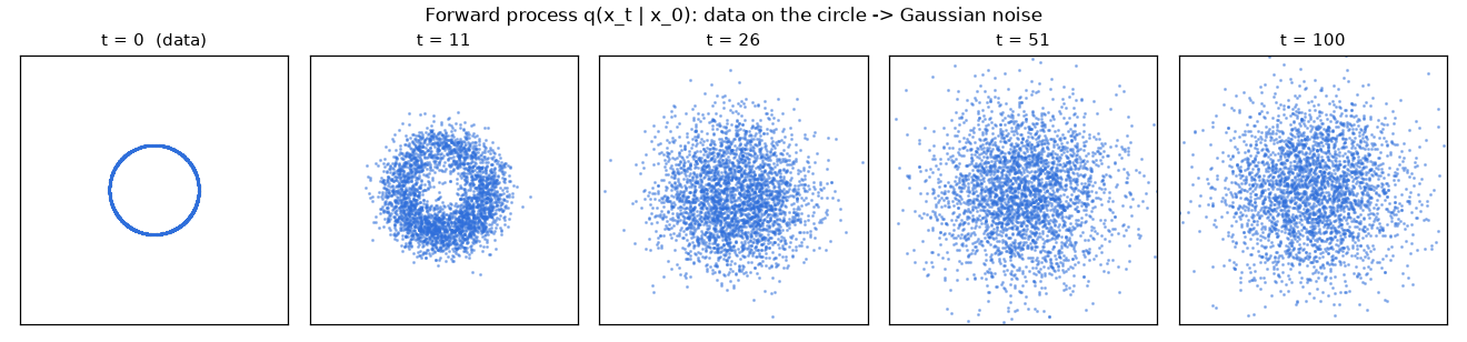
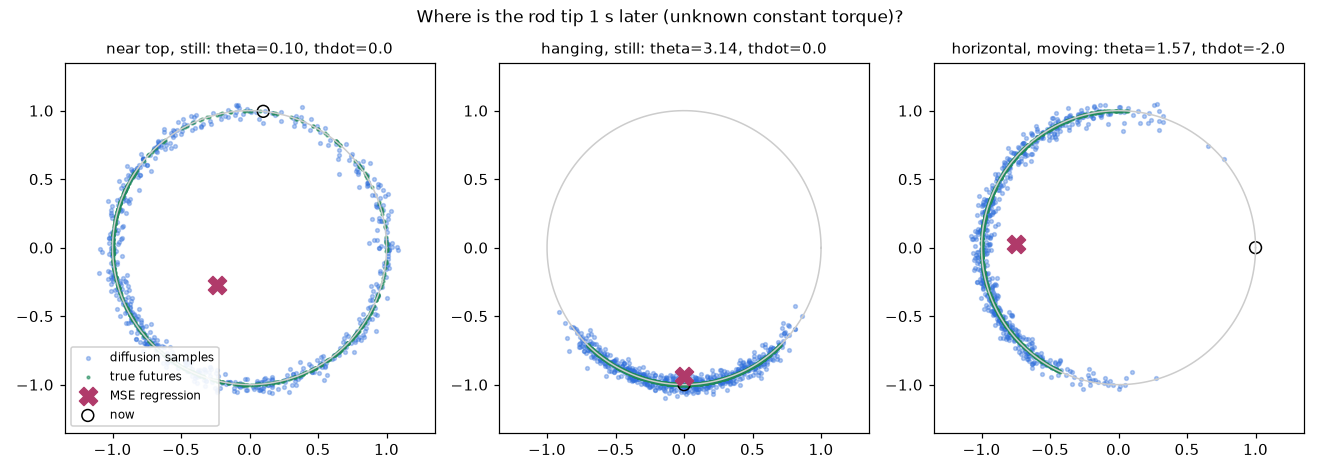
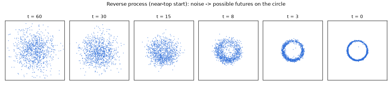
The prediction that minimizes MSE is the average of the possible futures (differentiating \(\mathbb{E}[(X - c)^2]\) with respect to \(c\) gives \(-2\mathbb{E}[X - c]\), and setting it to 0 gives \(c = \mathbb{E}[X]\)). When the future branches, the average resembles none of the branches. In a World Model that predicts pixels with MSE, this average shows up as a blurry image with several futures superimposed. A diffusion model draws a sample rather than the average, so it renders one sharp scene even when the future is uncertain. Making the latent variable stochastic in the RSSM is a different answer to the same problem.
DIAMOND and GameNGen
Real diffusion World Models put the last few images and actions in the condition slot and draw the entire next image from noise. \(k\) is the noise level and \(t\) is the environment time.
\(\epsilon_\theta\big( x^{(k)}_{t+1},\ k,\ o_{t-L+1}, \dots, o_t,\ a_{t-L+1}, \dots, a_t \big)\)
What the network predicts varies from paper to paper. GameNGen predicts the "velocity" \(v\), a mixture of noise and data (v-prediction), while DIAMOND uses the EDM formulation (Karras et al., 2022) instead of DDPM and predicts toward the clean image. Given \(x_t\), \(\epsilon\), \(x_0\), and \(v\) are interchangeable, so the skeleton of the derivation is the same. DIAMOND reports that using EDM is what made sampling with few steps possible.
Three names that come up often in large World Models since DDPM:
- Flow matching (Lipman et al., 2022): regresses a vector field (velocity) that says which direction and how far to move along a fixed probability path connecting noise and data. The idea is close to v-prediction.
- Diffusion forcing (Chen et al., 2024): trains the model to remove noise when each token (frame) in a sequence is given an independent noise level. With past frames clean and future frames starting from noise, it unifies "next-frame prediction" and "whole-sequence diffusion" in one model.
- Shortcut model (Frans, Hafner, Levine, Abbeel, 2024): conditions the network on both the noise level and the step size to skip at once, producing good samples in one or a few sampling steps without separate distillation. The shortcut forcing of Dreamer 4 is a training objective that combines this shortcut model with diffusion forcing.
The representative models are:
- DIAMOND (Alonso et al., NeurIPS 2024 Spotlight): trained an agent inside a diffusion World Model and reported a mean HNS of 1.46 (146%) on Atari 100k (the best at the time for an agent trained entirely inside a World Model). As its title "Visual Details Matter" suggests, it argues that diffusion has the edge when small visual details that vanish in discrete tokens or blurry reconstructions (such as small bullets) matter for action. The design was refined to use only a few denoising steps, and the same method was scaled up and applied to CS:GO footage.
- GameNGen (Valevski et al., 2024; ICLR 2025): recorded footage of a reinforcement learning agent playing DOOM and modified Stable Diffusion v1.4 to predict "past images + action → next image". It ran the game purely on a neural network at about 20 frames per second on a single TPU, and human raters could tell short clips of real and generated footage apart only slightly better than chance.
Beware of drift. During training the condition contains real past images, but during an imagined rollout the images the model generated itself become the next condition. Small errors fed back as the next input and growing larger is the same problem as the error accumulation in chapter 6. GameNGen deliberately added Gaussian noise to the conditioning images during training so the model would learn to correct itself after seeing a slightly wrong past, and reports that this was crucial for keeping the screen stable over long periods.
| Pros | Cons |
| Draws branching futures sharply (no blurring). Preserves small visual details well. Can build on proven technology from image and video generation. | Slow, since each image requires many denoising passes (steps × frames). Long-term consistency is hard (drift). Reward and value must be predicted separately. |
Predicting representations instead of pixels: JEPA
The idea
Details such as the position of leaves swaying in the wind or the shape of ripples are inherently unpredictable. Asked to predict pixels, a model either wastes capacity on such details or averages them into a blur. In his 2022 position paper "A Path Towards Autonomous Machine Intelligence", Yann LeCun proposed JEPA (Joint-Embedding Predictive Architecture). An input \(x\) and a target \(y\) are each turned into representations \(s_x, s_y\) by encoders, and prediction happens in representation space.
\(s_x = \text{Enc}_\theta(x), \qquad s_y = \text{Enc}_{\bar\theta}(y), \qquad \hat s_y = \text{Pred}_\theta(s_x,\ \text{condition}), \qquad E(x, y) = D\big(s_y,\ \hat s_y\big)\)
\(D\) is a distance (e.g. L1 or L2), and \(E(x, y)\) is called the energy. Training makes the energy low for matching pairs and high for mismatched ones. As a World Model, \(x\) is the current video, the condition is the action, and \(y\) is the future video. Because the encoder can leave unpredictable details out of the representation, the predictor can focus on the predictable essentials such as objects' positions and motion. Generative models (Dreamer, diffusion) regenerate pixels and compare pixels with pixels, while JEPA compares the representations produced by two encoders. The target-side encoder is an EMA target with stopped gradients.
Collapse and how to prevent it
If both encoders output the same constant vector \(\mathbf{c}\) for any input and the predictor also outputs \(\mathbf{c}\), then \(E(x, y) = D(\mathbf{c}, \mathbf{c}) = 0\) for every pair, matched or not. A model that distinguishes nothing achieves the lowest loss: this is representation collapse. Dreamer, with its reconstruction loss, does not have this problem, because the decoder cannot reconstruct different images from \(\mathbf{c}\). Ways to prevent it:
- Contrastive learning: deliberately raise the energy of mismatched pairs (negative samples). This requires many negative samples.
- EMA target encoder + stop-gradient: the target-side encoder \(\bar\theta\) is not trained; instead it slowly follows the trained encoder \(\theta\) as an exponential moving average (EMA): \(\bar\theta \leftarrow \tau\, \bar\theta + (1 - \tau)\, \theta\) with \(\tau \approx 0.99 \sim 0.999\). It originated with BYOL and is used by I-JEPA and V-JEPA.
- Variance and covariance regularization: penalize the representation unless each component is sufficiently spread out across samples (VICReg).
- Isotropic Gaussian regularization: LeJEPA (Balestriero & LeCun, November 2025) presented a theory that the best distribution for JEPA representations is an isotropic Gaussian (equal variance in every direction) and proposed SIGReg (sketched isotropic Gaussian regularization), a regularization term that pushes representations toward that distribution. If representations clump into a single point they move away from the Gaussian and are penalized. It reportedly uses neither stop-gradient nor a teacher-student (EMA) structure and has only one hyperparameter to tune.
Unrolling the EMA update rule all the way gives an exponentially weighted average of past values.
\(\begin{align} \bar\theta_n &= \tau\,\bar\theta_{n-1} + (1 - \tau)\,\theta_n \\ &= \tau^2 \bar\theta_{n-2} + (1-\tau)\big(\theta_n + \tau\,\theta_{n-1}\big) \\ &= (1 - \tau) \sum_{j=0}^{n-1} \tau^{j}\, \theta_{n-j} + \tau^{n}\, \bar\theta_0 \end{align}\)
More recent values receive larger weights. Because the target encoder does not change abruptly, it reduces the risk of the trained side chasing a moving target and collapsing along with it. Why this alone prevents collapse, however, has not been fully explained theoretically. With \(\tau = 0.9\), if the trained side suddenly changes from 1 to 0, the target follows slowly: \(0.9 \to 0.81 \to 0.729 \to 0.6561 \to 0.5905\).
The VICReg variance term penalizes the representation when the within-batch standard deviation of its \(j\)-th component falls below a threshold \(\gamma\) (usually 1).
\(v = \frac{1}{d}\sum_{j=1}^{d} \max\big(0,\ \gamma - \sqrt{\operatorname{Var}(s^{(j)}) + \varepsilon}\big)\)
Under collapse every component has zero variance, so the penalty reaches its maximum, \(\gamma - \sqrt{\varepsilon} \approx 1\), and the collapsed solution is no longer optimal.
I-JEPA, V-JEPA, V-JEPA 2, and smaller models
- I-JEPA (Assran et al., CVPR 2023): masks some blocks of an image and predicts the representations of the masked blocks from the representation of the visible part. It learns image representations without reconstructing pixels.
- V-JEPA (Bardes et al., 2024): extends the same idea to video, predicting the representations of regions masked in space and time.
- V-JEPA 2 (Meta, June 2025): pretrained an encoder of about 1 billion parameters on over 1 million hours of internet video, then trained an action-conditioned predictor, V-JEPA 2-AC, on top using less than 62 hours of robot video (the DROID dataset). It reported successfully planning to pick up and move objects given a goal image on Franka robot arms in two other labs, with no data from those environments (zero-shot).
- V-JEPA 2-AC plans the same way as CEM in chapter 7: it samples candidate action sequences, imagines future representations with the predictor, and picks the sequence whose distance (energy) to the goal image's representation is smallest. It plans from a goal image alone, without a reward function.
- DINO-WM (Zhou, Pan, LeCun, Pinto, November 2024): instead of learning a new encoder, it takes the patch features of a pretrained DINOv2 as is and learns only to predict the next patch features from offline trajectories. Without reconstructing images, it optimizes the action sequence at test time to find a path toward the goal image's features (zero-shot planning without a reward model).
- LeWorldModel (Maes, Le Lidec, Scieur, LeCun, Balestriero, March 2026): learns a JEPA World Model end to end from pixels without a pretrained encoder. The loss has only two terms, "next-embedding prediction" and "regularization pushing the latent toward a Gaussian distribution". It reported training a model of about 15 million parameters on a single GPU in a few hours, with planning up to 48 times faster than World Models that rely on large pretrained models. This means JEPA can be experimented with at roughly the scale of chapter 11.
| Pros | Cons |
| Efficient, because it ignores unpredictable details. Can be pretrained on large amounts of reward-free video. Can plan from a goal image alone. | Needs a mechanism to prevent collapse. The imagined future cannot be viewed as an image (a separate decoder has to be attached), which makes debugging hard. It is hard to verify whether the representation holds the information needed for action. |
Large-scale video and interactive World Models
Since around 2024, "World Model" has also been widely used for generative models trained on huge video datasets that render a matching world in real time as a person or agent controls it with a keyboard or text. They share roots with the World Model of this tutorial (a learned simulator for an agent) but differ in scale and purpose.
What counts as a World Model? By this tutorial's definition, a World Model takes an action and predicts what comes next. A video generation model that produces an entire clip from a single line of text has no action input, so on its own it cannot be used to ask about the consequences of actions. The models below are easier to place if judged by whether they "take an action (or control input) at every frame".
Genie: learning actions without action labels
Genie (Bruce et al., ICML 2024) is an 11B-parameter "generative interactive environment" trained on internet footage of 2D platform games (filtered down to about 30,000 hours). Internet videos do not record which buttons were pressed, so the actions themselves are learned from the video.
- Video tokenizer: turns video into VQ tokens.
- Latent action model (LAM): looks at past frames together with the next frame and extracts an "action" \(\tilde a_t\) that explains the change between them, using a VQ with a codebook of size 8. It is then trained to reconstruct the next frame from the past frames and \(\tilde a_t\) alone.
- Dynamics model: a Transformer that predicts the next frame's tokens from past tokens and the latent action.
The latent actions become action-like because of an information bottleneck. The maximum information 8 codes can carry is the entropy of the uniform distribution.
\(H(\tilde a) = -\sum_{i=1}^{8} p_i \log p_i \le \log 8 = 2.079\ \text{nats}, \qquad \log_2 8 = 3\ \text{bits}\)
Only 3 bits can pass per frame, far too little to carry the screen's details, so the model fills this narrow channel with the information that explains the most frame-to-frame change, such as "left, right, jump": in other words, the controls.
The dynamics model uses a spatiotemporal (ST) Transformer to save computation. With \(T\) frames and \(N\) tokens per frame, full attention between all tokens involves \((TN)^2\) pairs, but splitting it into attention within the same frame (spatial) and across times at the same position (temporal) gives \(T N^2 + N T^2\). With \(T = 16\) and \(N = 400\) this is \(40{,}960{,}000\) versus \(2{,}662{,}400\), about 15 times fewer.
Genie 2, Genie 3, Genie 4
- Genie 2 (Google DeepMind, December 2024): creates a 3D world from a single image that can be controlled with keyboard and mouse. DeepMind described it as an autoregressive latent diffusion model, said the world stays consistent for up to about a minute (most examples last 10 to 20 seconds), and said it remembers parts of the world that leave the screen and redraws them when they come back.
- Genie 3 (August 2025): announced as able to render a world described in text at 720p and 24 frames per second with real-time interaction, keep it consistent for several minutes, and trigger "world events" such as changing the weather or adding objects via text. In January 2026, Project Genie, an experimental service built on it, opened to some paid subscribers in the United States.
- Genie 4 (October 2026): released as a research preview. It was presented as generating matching audio for the world in real time and allowing scenes to be changed by text during a session. Detailed figures such as resolution and frame rate were not disclosed, and the announcement also acknowledged that details can degrade in long sessions.
Sora, Cosmos, and World Models for autonomous driving
- Sora (OpenAI, February 2024): its technical report "Video generation models as world simulators" argued that scaling up video generation models could make them simulators of the physical world. It is a diffusion Transformer that uses spacetime patches as tokens. The report also acknowledged that it fails to accurately model basic physical interactions such as glass shattering. Whether "scaling alone leads to an understanding of physics" remains an open debate.
- NVIDIA Cosmos (January 2025): a collection of World Foundation Models for developing physical AI such as robots and autonomous vehicles. It released diffusion-based and autoregressive (next-token prediction) models along with video tokenizers, and stated that about 20 million hours of video were used as training data. Its headline use case is developers fine-tuning on their own robot or vehicle data to generate synthetic data.
- GAIA-1, GAIA-2 (Wayve, 2023 and 2025): generative World Models for autonomous driving. GAIA-1 turned video, text, and actions into tokens and predicted the next token; GAIA-2 switched to latent diffusion and jointly generates multi-camera video conditioned on ego-vehicle motion, surrounding vehicles, weather, and road layout. They are used to create and test dangerous situations without encountering them in reality.
- UniSim (Yang et al., ICLR 2024 Outstanding Paper Award): learned a real-world simulator that emulates the visual outcomes of both high-level instructions such as "open the drawer" and low-level robot controls, and showed that policies trained only inside it transfer directly to the real world (zero-shot transfer).
The agent side: DayDreamer, Dreamer 4, World Action Models
- DayDreamer (Wu et al., CoRL 2022): trained the Dreamer of chapter 12 directly on real robots without a simulator. The A1 quadruped robot learned in about an hour, without resets, to roll over from lying on its back, stand up, and walk; a robot arm learned to pick and place objects from camera images and sparse rewards; and a wheeled robot learned to navigate to a goal from camera images alone. It showed that the sample efficiency of World Models matters in practice.
- Dreamer 4 (Hafner, Yan, Lillicrap, September 2025): a scalable Transformer World Model with a new training objective, shortcut forcing (which combines the shortcut model and diffusion forcing to generate the next frame in few sampling steps), allowing imagination rollouts in real time on a single GPU. It was reported as the first agent to obtain diamonds in Minecraft purely from offline data, without any interaction with the environment. Getting to a diamond takes a chain of more than 20,000 mouse and keyboard actions.
- World Action Model: DreamZero (Ye et al., February 2026): instead of using the World Model as a simulator for training a policy, it uses the World Model itself as the policy. Building on a pretrained video diffusion model, it is trained to predict future video and robot actions jointly. The idea is that predicting video requires knowing how the world moves, and that knowledge carries over to action prediction. In real robot experiments it reported more than twice the generalization to new tasks and environments compared with existing VLA (vision-language-action) models, and closed-loop control at 7 times per second with a 14-billion-parameter autoregressive video diffusion model. It marks the point where the line between chapter 7's "imagine with the model and choose" and chapter 12's "learn a separate policy" begins to blur.
Comparison of families
| Family | Representatives | What is predicted | Latent / representation | Training objective | How it is used | Data scale (approx.) |
| VAE + RNN | Ha & Schmidhuber (chapter 10) | Pixel reconstruction + next latent | Gaussian \(z\) + LSTM | VAE ELBO, MDN likelihood | Evolution strategies inside the dream | About 10,000 episodes (10,000 random rollouts) |
| RSSM | PlaNet, Dreamer (chapters 11 and 12) | Pixel reconstruction, reward | Deterministic \(h\) + stochastic \(z\) | Sequential ELBO | CEM planning / actor-critic in imagination | Hundreds of thousands to millions of steps |
| Value equivalence | MuZero, EfficientZero | Reward, value, policy | Hidden state (no decoder) | Loss unrolled over K steps | MCTS | Atari 100k to billions of frames |
| Decoder-free latent | TD-MPC2 | Reward, Q, next latent | SimNorm latent | Reward + TD + latent consistency | MPPI + Q | Hundreds of thousands to millions of steps per task |
| Tokens + Transformer | IRIS, TWM, STORM | Next token, reward | VQ tokens / categorical latent | Cross-entropy | Actor-critic in imagination | Atari 100k (about 2 hours) |
| Diffusion | DIAMOND, GameNGen | Next image (pixels) | Raw pixels or a latent | Denoising (ε, v, or x₀ prediction) | Learning in imagination / replacing a game engine | Atari 100k to large-scale gameplay recordings |
| Representation prediction | V-JEPA 2 | Future representation | Self-supervised representation | Representation distance + collapse prevention | CEM planning toward a goal image | Over 1 million hours of video, under 62 hours of robot data |
| Large-scale video | Genie, Sora, Cosmos, GAIA | Next frame, video | Video tokens, latents | Next token / diffusion | Simulator for people and agents, synthetic data | Tens of thousands to tens of millions of hours |
| World Action Model | DreamZero | Future video + actions | Latent of a video diffusion model | Joint denoising of video and actions | The model is the policy (executes the predicted actions) | Pretrained video model + robot data |
The pendulum revisited
How each family would handle the same pendulum problem:
- Dreamer (chapter 12): turns 64×64 images into RSSM latents and learns by reconstructing the images. The images are simple, with no background, so the reconstruction loss is not very wasteful.
- MuZero: sees the images but does not redraw them, predicting only reward, value, and policy. MCTS suits discrete actions, so the torque has to be discretized, e.g. into \(\{-2, -1, 0, 1, 2\}\). Early on it almost always receives large negative rewards, so the signal about which states are better is weak and the hidden state is hard to train (EfficientZero's consistency loss helps).
- TD-MPC: turns either the numeric state \([\cos\theta, \sin\theta, \dot\theta]\) or images into a latent, imagines only about 5 steps, and fills in the rest with Q. The MPC of chapter 7 imagined 25 steps.
- IRIS: turns a 64×64 image into 16 tokens. The pole spans only a few tokens, so success depends on whether small differences in angle are well distinguished by the tokens.
- Diffusion: this chapter's exercise shows what it looks like. Even when it is unknown which way an upright pendulum will fall, it draws one sharp branch of the future instead of a blurry average.
- JEPA: given "an image of the pole standing straight up" as the goal, it uses CEM to find a torque sequence that reduces the distance to that goal in representation space. No separate reward function needs to be defined.
- Genie-style learning: even with only pendulum videos and no torque logs, a latent action model would likely discover a handful of codes such as "push left, push right, hold still" on its own.
Open problems
- Long-horizon consistency: the error accumulation of chapter 6 does not go away even in huge models. It is hard enough that Genie 2, 3, and 4 extending consistency to the scale of "minutes" was itself announced as a major achievement.
- Understanding causality and physics: plausible-looking video and physically correct video are different things (Sora's glass example). A model that mispredicts the consequences of actions cannot be used for planning.
- Evaluation: high scores on generation-quality metrics (PSNR, measured by pixel error; FVD, measured by the distance between video distributions; and others) do not guarantee that a policy trained inside the model will actually work well. Methods that measure "does it look good?" and "is it useful?" together are lacking.
- Model exploitation: as seen in chapter 10, a policy finds gaps in the World Model (places where it differs from reality) and learns tricks that only work in the dream. Larger models have fewer gaps, but the gaps never disappear.
- Computational cost: the many denoising steps of diffusion models and the long context of Transformers make real-time interaction and learning in imagination expensive. Techniques for generating in few steps (such as the shortcut approach in Dreamer 4) are an active research area.
- Safety and transfer to the real world: in robotics and autonomous driving, failures where the World Model is wrong become real accidents. Uncertainty estimation (the ensembles of chapter 7) and conservative planning remain important.
Summary
- Modern World Models fall into place when sorted by what they predict, the shape of the latent, the tool connecting time steps, how they are used, and scale.
- MuZero: a value-equivalent model that predicts only reward, value, and policy, plus MCTS. The value target is the n-step return \(\sum_{i \lt n}\gamma^i r_{t+i} + \gamma^n v(s_{t+n})\).
- TD-MPC: learns without a decoder from reward + TD + latent consistency, and plans with short imagination + Q. The MPPI weight \(\exp(J/\tau)\) is the solution to maximizing "expected score − τ·KL".
- Transformer World Models: turn images into tokens with VQ (straight-through estimator) and predict the next token via the chain rule. Attention scores are divided by \(\sqrt{d}\) to bring their variance to 1.
- Diffusion World Models: \(x_t = \sqrt{\bar\alpha_t}x_0 + \sqrt{1-\bar\alpha_t}\epsilon\), reverse mean \(\frac{1}{\sqrt{\alpha_t}}(x_t - \frac{\beta_t}{\sqrt{1-\bar\alpha_t}}\epsilon)\), and training is noise-prediction MSE. They output samples rather than averages, so they do not blur.
- JEPA: predicts in representation space and discards unpredictable details. Collapse is prevented with an EMA target or variance regularization.
- Large-scale models (Genie, Sora, Cosmos, GAIA) only become World Models in this tutorial's sense when they take actions or controls at every frame; long-term consistency, physics, and evaluation remain open challenges.
Review questions
- Question 1. With \(\gamma = 0.5\), \(n = 2\), rewards \(r_t = 4\), \(r_{t+1} = 2\), and \(v(s_{t+2}) = 8\), what is the n-step target \(z_t\)?
- \(z_t = 4 + 0.5 \times 2 + 0.5^2 \times 8 = 4 + 1 + 2 = 7\).
- Question 2. Find the MPPI weights of two candidates with scores \(J = (3, 1)\) for \(\tau = 1\), \(\tau \to 0\), and \(\tau \to \infty\).
- For \(\tau = 1\), divide \((1,\ e^{-2}) = (1,\ 0.1353)\) by the sum \(1.1353\) to get \(w = (0.881,\ 0.119)\). As \(\tau \to 0\), the exponent in \(\exp((J_i - J_{\max})/\tau)\) goes to \(-\infty\) for every candidate other than the best, giving \(w = (1, 0)\), i.e. argmax. As \(\tau \to \infty\), all exponents go to 0, giving \(w = (0.5, 0.5)\), a plain average that ignores the scores.
- Question 3. What are the forward value of
z_tilde = z_e + (z_q - z_e).detach()and its gradient with respect toz_e, and what happens if.detach()is removed? - The value is \(z_e + z_q - z_e = z_q\) and the gradient is \(\partial \tilde z/\partial z_e = I\), so the gradient from the decoder passes straight to the encoder. Without
.detach(), \(\tilde z = z_q\), the gradient becomes \(\partial z_q / \partial z_e = 0\), and the encoder does not learn. - Question 4. If the components of the query and key are independent random variables with mean 0 and variance \(\sigma^2\), what should the score \(q \cdot k\) be divided by to make its variance 1?
- \(\operatorname{Var}(q_i k_i) = \mathbb{E}[q_i^2]\mathbb{E}[k_i^2] = \sigma^4\) and the variance of the sum is \(d\sigma^4\), so divide by \(\sigma^2\sqrt{d}\).
- Question 5. With \(\beta_1 = 0.2\), \(\beta_2 = 0.5\), and \(x_0 = 1\), find the mean and variance of \(q(x_2 \mid x_0)\).
- \(\alpha_1 = 0.8\), \(\alpha_2 = 0.5\), and \(\bar\alpha_2 = 0.4\), so the mean is \(\sqrt{0.4} = 0.632\) and the variance is \(0.6\). Following one step at a time gives the same result: \(\operatorname{Var}(x_1) = 0.2\), \(\operatorname{Var}(x_2) = 0.5 \times 0.2 + 0.5 = 0.6\).
- Question 6. In JEPA, what goes wrong if the target encoder shares the same parameters instead of being an EMA, with gradients flowing through both sides, and why do reconstruction-based models not have this problem?
- The two encoders move together and easily fall into the collapsed solution that maps every input to the same vector (energy 0 for every pair). A reconstruction-based model must recover the original image from the latent state, so mapping every input to the same latent makes the reconstruction loss large. The decoder prevents collapse.
See also
- World Models:Tutorial
- World Models
- World Models:Tutorial:12 Dreamer
- World Models:Tutorial:14 Appendix
- Genie (world model)
- GameNGen
- Sora
- Waymo World Model
- Physical AI
- Diffusion model
- Transformer
- VAE
- Reinforcement learning
Favorite site
- 13. The Modern World Model Landscape
- MuZero: Mastering Atari, Go, Chess and Shogi by Planning with a Learned Model (Schrittwieser et al.)
- EfficientZero: Mastering Atari Games with Limited Data (Ye et al.)
- TD-MPC (Hansen et al.)
- TD-MPC2
- VQ-VAE (van den Oord et al.)
- Transformer (Vaswani et al.)
- IRIS
- TWM
- STORM
- DDPM: Denoising Diffusion Probabilistic Models (Ho et al.)
- Flow matching (Lipman et al.)
- Diffusion forcing (Chen et al.)
- Shortcut model (Frans et al.)
- DIAMOND
- GameNGen
- A Path Towards Autonomous Machine Intelligence (LeCun)
- I-JEPA
- V-JEPA
- V-JEPA 2
- LeJEPA
- DINO-WM
- LeWorldModel
- Genie
- Genie 2 (DeepMind blog)
- Genie 3 (news report)
- Project Genie (news report)
- Genie 4 (Google blog)
- Genie (DeepMind model page)
- Video generation models as world simulators (OpenAI)
- NVIDIA Cosmos
- GAIA-1
- GAIA-2
- UniSim
- DayDreamer
- Dreamer 4
- DreamZero: World Action Models are Zero-shot Policies (Ye et al.)