WorldModels:Tutorial:12-Dreamer
lastmod 2026-11-18created 2026-11-172 edits
Dreamer: Learning Behaviors in Imagination is Chapter 12 of the World Model tutorial. Chapter 11's PlaNet imagines 120,000 steps inside the World Model for every decision and then throws them away; Dreamer uses the same imagination to train an actor (policy) and a critic (value function). This chapter derives imagined trajectories, the λ-return, the critic loss, actor training by differentiating through the World Model, and the entropy of a tanh-Gaussian policy. It then covers an implementation that swings a pendulum upright from pixels alone, along with measured results, and finally the techniques of DreamerV2 and DreamerV3.
- Original: 12. Dreamer: Learning Behaviors in Imagination
- Code:
code/ch12_dreamer.py(importsch11_rssm_planet.py; about 45 minutes with a laptop GPU to itself,--quicktakes about 15 seconds on CPU) - Previous: 11. RSSM and PlaNet / Next: 13. The Landscape of Modern World Models
The cost of planning and the idea behind Dreamer
PlaNet's planning has two weaknesses.
- It is expensive. Each decision rolls the RSSM forward \(I \times H \times J = 10 \times 12 \times 1000 = 120{,}000\) steps. Even on a laptop GPU, one decision took around 0.1 seconds. The imagined futures are discarded once a single action is chosen, and the next moment starts imagining from scratch.
- It is short-sighted. The planner only looks at the sum of rewards within \(H = 12\) steps. This can be fatal in problems like the pendulum, where a move that costs now (swinging down to build momentum) pays off greatly later (standing upright).
Two tools from Chapter 5 solve these problems.
- Policy (actor) \(\pi_\psi(a \mid s)\): a neural network that takes a state and outputs an action. Once trained, each decision needs only one forward pass. This solves the cost problem.
- Value function (critic) \(v_\xi(s)\): predicts the sum of future rewards from a state. Adding the value at the point where imagination ends lets the agent see beyond the horizon. This solves the short-sightedness problem.
Learning a policy and a value function usually takes a lot of experience (model-free reinforcement learning). Dreamer generates that experience by imagining with the World Model. Thousands of imagined rollouts can run in parallel on a GPU, and they never touch the real world.
Dreamer was introduced by Hafner, Lillicrap, Ba, and Norouzi in Dream to Control: Learning Behaviors by Latent Imagination (ICLR 2020). It reuses the RSSM from Chapter 11 as its World Model and adds behavior learning in imagination on top.
Three loops
| Loop | What it does |
| ① Model learning (same as Chapter 11) | Sample B×L chunks from the replay buffer D and train the RSSM with the sequential ELBO. This yields B·L posterior states. |
| ② Behavior learning in imagination (the new part) | From each posterior state, imagine H=15 steps with the actor and compute λ-returns. The critic is fit to the λ-returns, and the actor increases the λ-returns by differentiating through the model. |
| ③ Environment interaction | Update the belief state from images and act with the actor (+ noise). No planning, just one network pass. Add the new episode to D. |
One episode is collected every C=100 training steps. Loop ③ replaces PlaNet's CEM planning with a single pass of the actor network.
Building imagined trajectories
Imagination starts from the posterior states computed while training the World Model in ①. A batch is \(B = 50\) sequences × length \(L = 50\), giving 2,500 starting points.
- They are states inferred from scenes actually experienced, with the images taken into account, so they are the most trustworthy starting points.
- They are drawn from all over the buffer, so they mix moments when the pendulum hangs down, spins, and stands up.
- They have already been computed, so they cost nothing extra.
From a starting point \(s_0 = (h_0, z_0)\), imagine \(H = 15\) steps. Imagined time is counted as \(t = 0, 1, \dots, H\).
\(\begin{align} a_t &\sim \pi_\psi(a_t \mid s_t) \\ h_{t+1} &= f_\theta(h_t, z_t, a_t),\quad z_{t+1} \sim p_\theta(z_{t+1} \mid h_{t+1}) \\ \hat{r}_t &= R_\theta(h_{t+1}, z_{t+1}) \end{align}\)
The actor picks an action, the RSSM prior takes one step without images, and the reward is predicted at the resulting state. The critic also predicts a value \(v\) at each resulting state.
Mind the reward subscript. Chapter 11's reward model predicts "the reward received on arriving at state \(s_{t+1}\)" from \(s_{t+1}\). This chapter calls that value \(\hat{r}_t\). In other words, \(\hat{r}_t\) is the reward for taking \(a_t\) in \(s_t\), which uses the same subscript as \(r_t\) in Chapter 5, so Chapter 5's return formulas apply unchanged. Papers align this subscript slightly differently, so first check which state the reward is predicted from.
    def imagine(self, h, z):
        """사후 상태 (N, ·) 에서 출발해 액터로 H 스텝을 상상한다. 상태 · 엔트로피 목록을 돌려준다."""
        feats, ents = [self.wm.feat(h, z)], []
        for _ in range(self.cfg.imag_horizon):
            a, ent = self.actor.sample(feats[-1].detach())  # 액터 입력에서는 기울기를 끊는다 (sg)
            h, z, _, _ = self.wm.rssm.img_step(h, z, a)  # z ~ p(z | h) 도 재매개변수화로 뽑는다
            feats.append(self.wm.feat(h, z))
            ents.append(ent)
        return torch.stack(feats), torch.stack(ents)  # (H+1, N, F), (H, N)
-
img_stepis the function from Chapter 11. Sampling \(z\) from the prior also uses reparameterization, so the whole imagined trajectory is a differentiable computation. -
featshas shape(H+1, N, 230): \(s_0, \dots, s_H\) for each of the \(N = 2500\) trajectories.
Value estimation: from n-step returns to λ-returns
The discounted return from Chapter 5 is:
\(G_t = \hat{r}_t + \gamma\,\hat{r}_{t+1} + \gamma^2\,\hat{r}_{t+2} + \cdots = \sum_{k=0}^{\infty} \gamma^k\,\hat{r}_{t+k}\)
Imagination ends after \(H = 15\) steps, so everything after that point is replaced by the critic's prediction. This follows naturally from the definition of the value function, \(v(s) = \mathbb{E}[G \mid s]\).
n-step return
Summing \(n\) steps of imagined rewards and finishing with the critic gives the n-step return.
\(V^{(n)}_t = \sum_{k=0}^{n-1} \gamma^k\,\hat{r}_{t+k} + \gamma^n\, v(s_{t+n})\)
\(\begin{align} V^{(1)}_t &= \hat{r}_t + \gamma\, v(s_{t+1}) \\ V^{(2)}_t &= \hat{r}_t + \gamma\,\hat{r}_{t+1} + \gamma^2\, v(s_{t+2}) \\ V^{(3)}_t &= \hat{r}_t + \gamma\,\hat{r}_{t+1} + \gamma^2\,\hat{r}_{t+2} + \gamma^3\, v(s_{t+3}) \end{align}\)
\(n = 1\) is the right-hand side of the Bellman equation (the TD target). Choosing \(n\) is a tug-of-war between bias and variance.
| Small \(n\) (e.g., 1) | Large \(n\) (e.g., 15) | |
| Reliance on the critic | High. If the critic is wrong, so is the estimate (bias). | Low. The critic's weight shrinks to \(\gamma^{n}\). |
| Reliance on imagination (the model) | Low. Only one step is imagined. | High. Errors and randomness accumulate over a long imagined rollout (variance). |
| Early in training | Bad, because the critic is still poor. | Good, because reward signals propagate quickly. |
Definition of the λ-return
The λ-return is an average of n-step returns weighted by powers of \(\lambda\). Let \(N = H - t\) be the number of steps remaining until the end of imagination at time \(t\) (in this section \(N\) is the number of remaining steps, not the number of trajectories). Then
\(V^\lambda_t = (1 - \lambda)\sum_{n=1}^{N-1} \lambda^{n-1}\, V^{(n)}_t + \lambda^{N-1}\, V^{(N)}_t,\qquad \lambda \in [0, 1]\)
The shorter returns receive weights \((1-\lambda), (1-\lambda)\lambda, (1-\lambda)\lambda^2, \dots\), and the longest, the \(N\)-step return, receives all the remaining weight \(\lambda^{N-1}\). Using the geometric series sum \(\sum_{n=1}^{N-1}\lambda^{n-1} = \frac{1 - \lambda^{N-1}}{1 - \lambda}\), the weights sum to 1.
\((1-\lambda)\cdot\frac{1 - \lambda^{N-1}}{1 - \lambda} + \lambda^{N-1} = 1 - \lambda^{N-1} + \lambda^{N-1} = 1\)
So the λ-return is a weighted average of n-step returns.
- \(\lambda = 0\): \(V^\lambda_t = V^{(1)}_t\). Relies most on the critic.
- \(\lambda = 1\): \(V^\lambda_t = V^{(N)}_t\). Uses imagination all the way to the end.
- Dreamer uses \(\lambda = 0.95\). With \(N = 15\), the longest return gets weight \(0.95^{14} \approx 0.488\), so almost half the weight goes to "15 imagined steps + the value at the end."
From the definition to a recursion
Computing by the definition requires building \(N\) n-step returns at every time step. We derive a recursion that computes everything in one backward pass. First we need a recursive property of the n-step return. Pull the \(k=0\) term out of the sum in the definition, factor out \(\gamma\), and change the index to \(j = k - 1\).
\(\begin{align} V^{(n)}_t &= \hat{r}_t + \sum_{k=1}^{n-1}\gamma^k\,\hat{r}_{t+k} + \gamma^n\, v(s_{t+n}) \\ &= \hat{r}_t + \gamma\left[\sum_{j=0}^{n-2}\gamma^{j}\,\hat{r}_{t+1+j} + \gamma^{n-1}\, v(s_{t+1+(n-1)})\right] \\ &= \hat{r}_t + \gamma\, V^{(n-1)}_{t+1},\qquad V^{(0)}_{t+1} := v(s_{t+1}) \end{align}\)
The bracket is exactly the definition of the \((n-1)\)-step return starting at time \(t+1\). Defining the "0-step return" as the critic value makes this hold for \(n = 1\) as well.
Substitute this property into the definition of the λ-return (\(N \ge 2\)).
\(\begin{align} V^\lambda_t &= (1 - \lambda)\sum_{n=1}^{N-1} \lambda^{n-1}\big[\hat{r}_t + \gamma V^{(n-1)}_{t+1}\big] + \lambda^{N-1}\big[\hat{r}_t + \gamma V^{(N-1)}_{t+1}\big] \\ &= \hat{r}_t\underbrace{\left[(1-\lambda)\sum_{n=1}^{N-1}\lambda^{n-1} + \lambda^{N-1}\right]}_{=\,1} + \gamma\left[(1-\lambda)\sum_{n=1}^{N-1}\lambda^{n-1} V^{(n-1)}_{t+1} + \lambda^{N-1} V^{(N-1)}_{t+1}\right] \\ &= \hat{r}_t + \gamma\left[(1-\lambda)\, V^{(0)}_{t+1} + (1-\lambda)\sum_{n=2}^{N-1}\lambda^{n-1} V^{(n-1)}_{t+1} + \lambda^{N-1} V^{(N-1)}_{t+1}\right] \\ &= \hat{r}_t + \gamma\left[(1-\lambda)\, v(s_{t+1}) + \lambda\left\{(1-\lambda)\sum_{m=1}^{N-2}\lambda^{m-1} V^{(m)}_{t+1} + \lambda^{N-2} V^{(N-1)}_{t+1}\right\}\right] \\ &= \hat{r}_t + \gamma\Big[(1-\lambda)\, v(s_{t+1}) + \lambda\, V^\lambda_{t+1}\Big] \end{align}\)
The justification for each line:
- Group the terms containing \(\hat{r}_t\) and the terms containing \(\gamma\). The coefficient of \(\hat{r}_t\) is the sum of the weights, 1.
- Pull the \(n = 1\) term, \((1-\lambda)\lambda^{0} V^{(0)}_{t+1}\), out of the sum.
- Replace \(V^{(0)}_{t+1}\) with \(v(s_{t+1})\), factor one \(\lambda\) out of the remaining two terms, and change the index to \(m = n - 1\).
- At time \(t+1\) the number of remaining steps is \(N - 1\), so the braces contain the definition with \(N\) replaced by \(N-1\), that is, \(V^\lambda_{t+1}\).
The terminal condition is \(V^\lambda_H := v(s_H)\). At \(t = H - 1\) (\(N = 1\)) the definition gives \(V^\lambda_{H-1} = \hat{r}_{H-1} + \gamma v(s_H)\), and plugging the terminal condition into the recursion gives the same, \(\hat{r}_{H-1} + \gamma[(1-\lambda)v(s_H) + \lambda v(s_H)]\).
Key result: the λ-return recursion
\(V^\lambda_t = \hat{r}_t + \gamma\Big[(1-\lambda)\, v(s_{t+1}) + \lambda\, V^\lambda_{t+1}\Big],\qquad V^\lambda_H = v(s_H)\)
Read it as "current reward + discounted [mix of the next state's critic value and the next state's λ-return in the ratio \((1-\lambda) : \lambda\)]." With \(\lambda = 0\) it becomes the one-step target \(\hat{r}_t + \gamma v(s_{t+1})\); with \(\lambda = 1\) it becomes Chapter 5's return recursion \(\hat{r}_t + \gamma V_{t+1}\).
Numerical check
Let \(H = 3\), \(\gamma = 0.9\), \(\lambda = 0.5\), rewards \(\hat{r}_0 = 1,\ \hat{r}_1 = 0,\ \hat{r}_2 = 2\), and critic values \(v(s_1) = 4,\ v(s_2) = 3,\ v(s_3) = 5\).
Recursion (from the back):
\(\begin{align} V^\lambda_3 &= 5 \\ V^\lambda_2 &= 2 + 0.9\,[0.5 \cdot 5 + 0.5 \cdot 5] = 6.5 \\ V^\lambda_1 &= 0 + 0.9\,[0.5 \cdot 3 + 0.5 \cdot 6.5] = 0.9 \cdot 4.75 = 4.275 \\ V^\lambda_0 &= 1 + 0.9\,[0.5 \cdot 4 + 0.5 \cdot 4.275] = 1 + 0.9 \cdot 4.1375 = 4.72375 \end{align}\)
Definition (\(t = 0\), \(N = 3\), weights 0.5, 0.25, 0.25):
\(\begin{align} V^{(1)}_0 &= 1 + 0.9 \cdot 4 = 4.6 \\ V^{(2)}_0 &= 1 + 0.9 \cdot 0 + 0.81 \cdot 3 = 3.43 \\ V^{(3)}_0 &= 1 + 0 + 0.81 \cdot 2 + 0.729 \cdot 5 = 6.265 \\ V^\lambda_0 &= 0.5 \cdot 4.6 + 0.25 \cdot 3.43 + 0.25 \cdot 6.265 = 2.3 + 0.8575 + 1.56625 = 4.72375 \end{align}\)
The two values match. The code computes with the recursion and also keeps a function that computes by the definition, comparing the two on every run.
def lambda_return(rewards, values, gamma, lam):
    """λ-리턴을 뒤에서부터 재귀식으로 계산한다.

    rewards : (H, N)    r̂_0 … r̂_{H-1}   (r̂_t = 상태 s_{t+1} 에서 예측한, 전이 t 의 보상)
    values  : (H+1, N)  v(s_0) … v(s_H)
    반환    : (H, N)    V^λ_0 … V^λ_{H-1}
      V^λ_t = r̂_t + γ [ (1-λ) v(s_{t+1}) + λ V^λ_{t+1} ],   V^λ_H = v(s_H)
    """
    H = rewards.shape[0]
    g = values[H]  # V^λ_H = v(s_H)
    out = []
    for t in reversed(range(H)):
        g = rewards[t] + gamma * ((1 - lam) * values[t + 1] + lam * g)
        out.append(g)
    return torch.stack(out[::-1])
The function that computes by the definition (lambda_return_by_definition) is in the lambda-check section of ch12_dreamer.py. Running the script prints the maximum difference between the two results.
On random rewards and values, the two computations differ by about \(10^{-7}\) (rounding error of 32-bit floats).
Critic learning
The critic \(v_\xi(s)\) learns to predict the λ-return of imagined states \(s_t\). The λ-return is a bootstrapped target built from the critic's own values, so the gradient is blocked on the target side.
\(\mathcal{L}(\xi) = \mathbb{E}\left[\sum_{t=0}^{H-1} \frac{1}{2}\Big(v_\xi(s_t) - \operatorname{sg}\big(V^\lambda_t\big)\Big)^2\right]\)
\(\operatorname{sg}(\cdot)\) is stop-gradient: the value is used as is but treated as a constant when differentiating. In PyTorch it is .detach(). Since \(\frac{\partial}{\partial \xi}\operatorname{sg}(V^\lambda_t) = 0\), the gradient is:
\(\frac{\partial}{\partial \xi}\,\frac{1}{2}\big(v_\xi(s_t) - \operatorname{sg}(V^\lambda_t)\big)^2 = \big(v_\xi(s_t) - V^\lambda_t\big)\cdot\frac{\partial v_\xi(s_t)}{\partial \xi}\)
This is plain regression: decrease the prediction if it is above the target and increase it if below. Without the block, gradients would also flow through \(v_\xi(s_{t+1})\) inside \(V^\lambda_t\), giving the critic a way to reduce the loss by pulling the target toward itself.
Two more stabilizers are used.
- Slow critic (target critic): the \(v\) used to compute λ-returns is not the critic being trained but a copy refreshed once every 100 training steps. This keeps the target from shifting at every step. It was introduced in DreamerV2 and is absent from the original DreamerV1. It is the same idea as the DQN target network in Chapter 5.
- Input blocking: the states fed to the critic are also cut with
feats[:-1].detach()so the critic loss does not affect the World Model or the actor.
Actor learning: differentiating through the World Model
The actor's goal is to increase the λ-return in imagination. Flip the sign to make it a loss and add an entropy bonus for exploration.
\(\max_\psi\ \mathbb{E}\left[\sum_{t=0}^{H-1} V^\lambda_t\right] \quad\Longrightarrow\quad \mathcal{L}(\psi) = -\,\mathbb{E}\left[\sum_{t=0}^{H-1} V^\lambda_t\right] - \eta\,\mathbb{E}\left[\sum_{t=0}^{H-1}\mathcal{H}\big[\pi_\psi(\cdot \mid s_t)\big]\right]\)
\(\mathcal{H}\) is the entropy of the policy. Following the Dreamer paper, \(\eta\) in this chapter denotes the entropy coefficient, not the learning rate.
REINFORCE and reparameterization gradients
The policy gradient theorem from Chapter 5 (the log-derivative trick) is:
\(\nabla_\psi\, \mathbb{E}_{a \sim \pi_\psi}[R(a)] = \mathbb{E}_{a \sim \pi_\psi}\big[R(a)\,\nabla_\psi \log \pi_\psi(a \mid s)\big]\)
This formula uses only the value of the return \(R\), not how \(R\) changes with the action (its derivative). That makes it usable in real environments that cannot be differentiated, at the cost of high-variance estimates that need many samples.
The imagined world is a neural network. The GRU, the prior MLP, the reward model, and the critic are all differentiable, and sampling was done with reparameterization. Actions are sampled with reparameterization too.
\(a_t = \tanh\big(\mu_\psi(s_t) + \sigma_\psi(s_t)\,\epsilon_t\big),\qquad \epsilon_t \sim \mathcal{N}(0, 1)\)
The λ-return then becomes a differentiable function of \(\psi\). Following the computation graph \(\psi\) → action \(a_t\) → next state \(s_{t+1}\) → reward \(\hat{r}_t\) and value \(v(s_{t+1})\) → λ-return backward with backpropagation yields the gradient. This is what "backpropagate through the dynamics" means.
A one-step toy example. Let \(s_1 = s_0 + a_0\), \(\hat{r}_0 = -s_1^2\), \(v(s) = -2s^2\), and \(a_0 = \mu\) (no noise). With \(H = 1\), the λ-return is just \(V^{(1)}_0\).
\(\begin{align} V^\lambda_0 &= \hat{r}_0 + \gamma\, v(s_1) = -s_1^2 - 2\gamma s_1^2 \\ \frac{dV^\lambda_0}{d\mu} &= \frac{\partial V^\lambda_0}{\partial s_1}\cdot\frac{\partial s_1}{\partial a_0}\cdot\frac{\partial a_0}{\partial \mu} = (-2s_1 - 4\gamma s_1)\cdot 1 \cdot 1 \end{align}\)
This is the state derivative of the reward model and critic × the action derivative of the dynamics × the parameter derivative of the policy. With \(s_0 = 1,\ \mu = 0.2,\ \gamma = 0.9\), we get \(s_1 = 1.2\) and a gradient of \(-2.4 - 4.32 = -6.72\). It is negative, so increasing the return requires decreasing \(\mu\). Numerical check: with \(\mu = 0.21\), \(V^\lambda_0 = -1.4641 - 2.6354 = -4.0995\), worse than \(-4.032\) at \(\mu = 0.2\), and the rate of change \((-4.0995 + 4.032)/0.01 \approx -6.75\) nearly matches the derivative. A single computation tells you which way to adjust and by how much. With REINFORCE, getting the same information would require trying many actions and comparing their scores.
Key point. The real world (the physics of the pendulum) is a black box that cannot be differentiated, but the World Model is a neural network that is differentiable end to end. That is how Dreamer obtains an analytic gradient: "changing the action by this much changes the future return by this much." The price is that where the model is wrong, the gradient is wrong too, so the actor can exploit the model's errors. This is why real data must keep being collected to correct the model.
What gets updated and what is stopped
The gradient of the actor loss flows back through the entire imagined trajectory, but only the actor's parameters \(\psi\) should be updated.
| Location | Treatment | Reason |
| Starting point of imagination \(s_0\) | | The starting point is a constant determined by the data. This keeps the actor loss from affecting World Model learning (the posterior). |
| World Model parameters \(\theta\) | | The principle is that the model learns only from data. The actor optimizer holds only actor parameters, so the model would not change even without freezing, but freezing skips computing gradients for the model parameters, which is faster and leaves no chance for actor-loss gradients to mix into the model's |
| Slow critic parameters | | Gradients must flow through \(v(s_{t+1})\) to the states, but the critic itself must not change. |
| Actor input state | | Same as the public DreamerV1 code (an implementation choice not visible in the paper's equations). Only the gradient along "action \(a_t\) → subsequent states → rewards and values" remains; the path where \(a_t\) changes \(s_{t+1}\) and thereby the next action \(a_{t+1} = \pi_\psi(s_{t+1})\) (\(\partial a_{t+1}/\partial s_{t+1}\)) is ignored. It is an approximation that drops this term from the exact total derivative. |
| Critic target \(V^\lambda_t\) | | A bootstrapped target is a constant. |
| Critic input state | | Keeps the critic loss from affecting the imagined trajectory (the actor and the model). |
Freezing versus detaching. requires_grad_(False) only skips computing gradients for those parameters; it does not block gradients flowing through the layer toward its inputs. .detach() cuts the computation graph at that tensor, so no gradient flows past it at all. In actor learning, the World Model must be frozen, not detached. Detaching would hide the effect of actions on the future.
tanh-Gaussian policy
The pendulum's action (torque) lies in \([-2, 2]\). It is normalized to \([-1, 1]\) and multiplied by 2 when passed to the environment. A value \(u\) sampled from a Gaussian is squashed with \(\tanh\) into \((-1, 1)\).
class Actor(nn.Module):
    """tanh-가우시안 정책: u ~ N(μ, σ²), a = tanh(u) ∈ (-1, 1)."""

    def __init__(self, feat_dim, act_dim=1, hidden=300, layers=3, init_std=1.0, min_std=1e-4):
        super().__init__()
        self.net = mlp(feat_dim, hidden, 2 * act_dim, layers)
        self.raw_init_std = math.log(math.exp(init_std) - 1)  # softplus(raw) = init_std 가 되는 raw
        self.min_std = min_std

    def forward(self, feat):
        mean, std = self.net(feat).chunk(2, -1)
        mean = 5 * torch.tanh(mean / 5)  # 평균이 너무 커져 tanh 가 포화되지 않게 [-5, 5] 로 부드럽게 묶는다
        std = F.softplus(std + self.raw_init_std) + self.min_std
        return mean, std

    def sample(self, feat):
        """재매개변수화로 행동을 뽑고, 그 행동의 엔트로피 추정값도 함께 돌려준다."""
        mean, std = self(feat)
        eps = torch.randn_like(mean)
        u = mean + std * eps  # 기울기가 mean · std 로 흐른다
        a = torch.tanh(u)
        # H[a] = H[u] + E[log |da/du|],  log |da/du| = log(1 - tanh²(u))
        gauss_ent = (0.5 * math.log(2 * math.pi * math.e) + torch.log(std)).sum(-1)
        log_det = torch.log(1 - a.pow(2) + 1e-6).sum(-1)
        return a, gauss_ent + log_det

    def mode(self, feat):
        mean, _ = self(feat)
        return torch.tanh(mean)
-
mean = 5 * torch.tanh(mean / 5): softly bounds the mean to \([-5, 5]\). Since \(\tanh(5) \approx 0.9999\), larger values are meaningless, and if the mean grows too large, \(\tanh\) saturates and the gradient vanishes (the DreamerV1 approach). -
F.softplus(std + self.raw_init_std): adds the inverse-softplus value \(\log(e^1 - 1) \approx 0.541\) so that the standard deviation isinit_std(=1) when the initial output is near 0. -
mode()is the deterministic action \(\tanh(\mu)\) used for evaluation.
Entropy bonus and change of variables
If the actor commits to a single action too early, it stops trying new things. Subtracting \(\eta\,\mathcal{H}\) from the loss (increasing entropy) keeps exploration going. The entropy of the distribution transformed by \(a = \tanh(u)\) is found with the change-of-variables formula, starting from \(p_a(a)\,\vert da\vert = p_u(u)\,\vert du\vert\) (\(\tanh\) is increasing, so the mapping is one-to-one).
\(\begin{align} p_a(a) &= \frac{p_u(u)}{\left\vert \frac{da}{du} \right\vert} \\ -\log p_a(a) &= -\log p_u(u) + \log\left\vert \frac{da}{du} \right\vert \\ \mathcal{H}[a] &= \mathbb{E}[-\log p_a(a)] = \mathcal{H}[u] + \mathbb{E}\left[\log\left\vert \frac{da}{du} \right\vert\right] \end{align}\)
\(\frac{d}{du}\tanh(u) = 1 - \tanh^2(u) = 1 - a^2\) always lies between 0 and 1, so its log is at most 0. Squashing with \(\tanh\) compresses values into \((-1, 1)\) and reduces entropy. Using \(\mathbb{E}[(u-\mu)^2] = \sigma^2\), the Gaussian entropy is:
\(\mathcal{H}[u] = \mathbb{E}\left[\frac{1}{2}\log(2\pi\sigma^2) + \frac{(u-\mu)^2}{2\sigma^2}\right] = \frac{1}{2}\log(2\pi\sigma^2) + \frac{1}{2} = \frac{1}{2}\log(2\pi e\,\sigma^2)\)
The second expectation is approximated with the single action just sampled (Monte Carlo).
\(\mathcal{H}[a] \approx \sum_{\text{dim}}\left[\frac{1}{2}\log(2\pi e) + \log\sigma\right] + \sum_{\text{dim}}\log\big(1 - a^2\big)\)
This is gauss_ent + log_det in the code (\(10^{-6}\) is a small constant to avoid \(\log 0\)). With \(\sigma = 1\) the first part is \(\frac{1}{2}\log(2\pi e) \approx 1.419\). The entropy of a continuous distribution (differential entropy) can be negative, so a negative ent in the training log is normal.
The coefficient \(\eta\) is kept small at \(10^{-4}\). The original DreamerV1 used no entropy bonus and explored by adding noise \(\mathcal{N}(0, 0.3^2)\) to actions during collection; later versions use an entropy bonus. This implementation uses both.
Full algorithm
데이터 D ← 무작위 행동 에피소드 S 개
되풀이:
    C 번 되풀이:
        # ① 모델 학습 (11장)
        D 에서 B×L 조각 → 순차 ELBO 로 θ, φ 한 스텝 → 사후 상태 {(h, z)} B·L 개
        # ② 상상 속 행동 학습
        출발점 s_0 ← 사후 상태들 (기울기 차단)
        t = 0..H-1:  a_t ~ π_ψ(·|sg(s_t)),  s_{t+1} ← RSSM 사전(s_t, a_t),  r̂_t ← R(s_{t+1})
        V^λ_t ← 뒤에서부터 재귀식 (느린 크리틱 v 사용)
        액터:   ψ ← ψ − α_ψ ∇_ψ [ −mean(V^λ) − η·mean(H[π]) ]   (World Model 을 거슬러 역전파)
        크리틱: ξ ← ξ − α_ξ ∇_ξ mean( ½ (v_ξ(sg(s_t)) − sg(V^λ_t))² )
        100 번마다 느린 크리틱 ← 크리틱
    # ③ 환경과 상호작용
    에피소드 하나: 매 결정마다 그림으로 (h, z) 갱신 → a ~ π_ψ + 잡음 N(0, 0.3²) → 실행
    D 에 추가
    def train_step(self, batch):
        cfg = self.cfg
        # ① World Model: 11장과 똑같이 순차 ELBO 로 한 스텝
        wm_loss, metrics, states = self.wm.loss(batch)
        self.wm_opt.zero_grad(set_to_none=True)
        wm_loss.backward()
        nn.utils.clip_grad_norm_(self.wm.parameters(), cfg.grad_clip)
        self.wm_opt.step()

        # ② 상상: 배치의 모든 사후 상태 (B·L 개) 에서 출발. 출발점은 상수로 본다 (detach).
        h = states["h"].detach().reshape(-1, cfg.deter)
        z = states["z"].detach().reshape(-1, cfg.stoch)
        self.wm.requires_grad_(False)  # 액터 손실이 World Model 을 고치지 않게 얼린다 (기울기는 통과)
        feats, ents = self.imagine(h, z)
        rewards = self.wm.reward(feats[1:]).squeeze(-1)  # (H, N): r̂_t = R(s_{t+1})
        values = self.slow_critic(feats).squeeze(-1)  # (H+1, N): v(s_0..s_H)
        returns = lambda_return(rewards, values, cfg.gamma, cfg.lam)  # (H, N)
        self.wm.requires_grad_(True)

        # ③ 액터: λ-리턴을 키우는 쪽으로 (동역학을 거슬러 역전파) + 엔트로피 보너스
        if cfg.return_norm:  # DreamerV3: 리턴의 5–95 백분위 폭으로 나눈다 (1 보다 작으면 1)
            with torch.no_grad():
                q = torch.quantile(returns.flatten(), torch.tensor([0.05, 0.95], device=returns.device))
                self.ret_scale = 0.99 * self.ret_scale + 0.01 * (q[1] - q[0]).item()
            actor_obj = returns / max(1.0, self.ret_scale)
        else:
            actor_obj = returns
        actor_loss = -actor_obj.mean() - cfg.entropy_scale * ents.mean()
        self.actor_opt.zero_grad(set_to_none=True)
        actor_loss.backward()
        nn.utils.clip_grad_norm_(self.actor.parameters(), cfg.grad_clip)
        self.actor_opt.step()

        # ④ 크리틱: v(s_t) 를 λ-리턴(상수로 본다)에 맞춘다
        v = self.critic(feats[:-1].detach()).squeeze(-1)  # (H, N)
        critic_loss = 0.5 * ((v - returns.detach()) ** 2).mean()
        self.critic_opt.zero_grad(set_to_none=True)
        critic_loss.backward()
        nn.utils.clip_grad_norm_(self.critic.parameters(), cfg.grad_clip)
        self.critic_opt.step()

        # ⑤ 느린 크리틱: 일정 횟수마다 지금 크리틱을 복사 (목표값을 흔들리지 않게)
        self.steps += 1
        if self.steps % cfg.slow_critic_every == 0:
            self.slow_critic.load_state_dict(self.critic.state_dict())

        metrics.update(actor=actor_loss.item(), critic=critic_loss.item(),
                       imag_return=returns.mean().item(), entropy=ents.mean().item())
        return metrics
Within one train_step, three optimizers (World Model, actor, critic) each take one step on their own loss. The span between self.wm.requires_grad_(False) and (True) is where imagination runs with the World Model frozen. The collection and evaluation loops are in the main section of ch12_dreamer.py (collection uses actor.sample, evaluation uses actor.mode).
Hyperparameters
@dataclass
class DreamerConfig(Config):
    # 11장의 Config(모델 크기 · 배치 · 자유 내트 등)를 물려받고, 행동 학습에 필요한 값만 더한다.
    imag_horizon: int = 15  # H: 상상 길이
    gamma: float = 0.99  # γ: 할인율
    lam: float = 0.95  # λ: λ-리턴의 섞는 비율
    actor_lr: float = 8e-5
    critic_lr: float = 8e-5
    ac_hidden: int = 300  # 액터 · 크리틱 MLP 너비
    ac_layers: int = 3
    entropy_scale: float = 1e-4  # η: 엔트로피 보너스
    init_std: float = 1.0  # 액터의 처음 표준편차 (tanh 앞)
    slow_critic_every: int = 100  # 목표(느린) 크리틱을 몇 번마다 복사할지 (DreamerV2)
    return_norm: bool = False  # DreamerV3 식 리턴 정규화
| Name | Meaning | This implementation | DreamerV1 paper |
| World Model | RSSM, encoder, decoder, reward | Same as Chapter 11 (h 200, z 30, free nats 3) | Same |
| \(H\) | Imagination horizon | 15 | 15 |
| \(\gamma\) / \(\lambda\) | Discount / λ-return | 0.99 / 0.95 | 0.99 / 0.95 |
| Learning rate | Model / actor / critic | \(6\times10^{-4}\) / \(8\times10^{-5}\) / \(8\times10^{-5}\) | Same |
| \(B \times L\) | Batch | 50 × 50 | 50 × 50 |
| Actor, critic | MLP | Width 300, 3 hidden layers, ELU | ELU MLP of similar size |
| Gradient clipping | Norm limit | 100 | 100 |
| Exploration noise | During collection | 0.3 | 0.3 |
| Entropy \(\eta\) | Bonus coefficient | \(10^{-4}\) | None (explores via noise) |
| Slow critic | Copy interval | 100 steps | None (from V2 onward) |
| \(S\), \(C\), action repeat | Seed episodes, training steps, repeat | 5, 100, 2 | 5, 100, 2 |
| Reward scale | Reward magnitude for training | 0.1 | None (DMC rewards are already 0 to 1) |
Why the reward scale matters. The pendulum's reward can drop as low as \(-33\) per decision, and with \(\gamma = 0.99\) values reach the hundreds to thousands. The critic output starts near 0 and moves slowly at a learning rate of \(8\times10^{-5}\), so just reaching such values takes a long time. Multiplying rewards by 0.1 brings values to roughly the same magnitude as in DMC (the tasks DreamerV1 was evaluated on). DreamerV3 solves this problem with symlog and return normalization.
Results
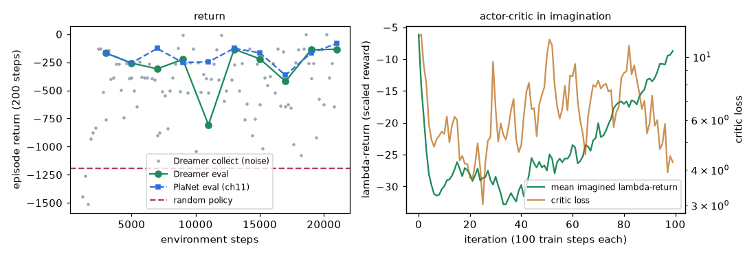
These are results with the default settings on a laptop GPU (8 GB), using the same seed and the same number of environment steps (21,000) as Chapter 11's PlaNet. The two training runs shared the GPU. imag G is the mean λ-return over imagined trajectories (with the 0.1 reward scale applied), ent is the actor's entropy estimate, and act is the time per decision in the real environment.
lambda-return check: recursion vs definition max |diff| = 2.38e-07
random policy return: -1194.5
it   1 | env steps   1200 | recon   78.5 kl 1.15 | imag G   -6.12 critic 11.788 ent -1.21 | return  -1445.7 | act  8.5 ms |    66s
it   2 | env steps   1400 | recon   23.8 kl 4.60 | imag G  -14.08 critic 12.012 ent -2.91 | return  -1257.8 | act  4.7 ms |   119s
it   3 | env steps   1600 | recon    5.9 kl 3.14 | imag G  -19.05 critic  9.342 ent -3.36 | return  -1513.0 | act 12.8 ms |   180s
…
it  10 | env steps   3000 | recon    1.9 kl 2.78 | imag G  -30.42 critic  5.457 ent -5.15 | return   -759.9 | act  2.7 ms |   598s | eval   -167.8
…
it  50 | env steps  11000 | recon    0.7 kl 2.67 | imag G  -26.70 critic  7.834 ent -6.87 | return   -520.6 | act  5.0 ms |  2529s | eval   -805.8
…
it 100 | env steps  21000 | recon    0.4 kl 2.62 | imag G   -8.73 critic  4.260 ent -6.90 | return   -129.7 | act  4.3 ms |  4799s | eval   -134.5
final eval over 10 episodes: mean -196.4, std 120.9, min -393.3, max -3.3
done in 4806s
The evaluation returns measured every 10 iterations (mean of 3 noise-free episodes) were, in order, −167.8, −257.7, −307.9, −224.8, −805.8, −133.4, −219.4, −419.3, −138.4, and −134.5.
Learning curves
- Figure: Return curves of Dreamer and PlaNet, imagined λ-return, and critic loss
- Same start. At 3,000 environment steps Dreamer reaches an evaluation return of −168, starting to swing the pendulum up at almost the same pace as PlaNet (−166). By this point the actor had experienced only 10 episodes in the real environment, but about \(100 \times 10 \times 2500 \times 15 \approx\) 37.5 million steps in imagination.
- More fluctuation. The evaluation return drops to −806 at 11,000 steps and then recovers. Planning (PlaNet) re-optimizes at every moment, so small changes in the model do not swing the result much, but the actor can end up learning the errors of the model and critic as well (model exploitation). The collection returns, with exploration noise, are also more scattered than PlaNet's.
- The imagined return rises late. The λ-return stays around −30 (−26 to −33) for the first 40 or so iterations and then climbs to −9. The early drop from −6 to −30 over the first few iterations happens because the reward model and critic initially output meaningless values near 0 and then learn the true (negative) rewards.
Episodes and imagination quality
- Figure: An episode in which the Dreamer policy swings the pendulum upright (return −135)
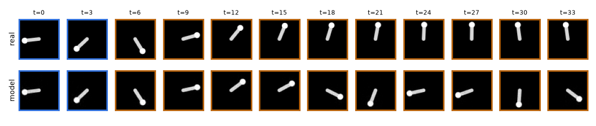
- Figure: Imagined vs. real frames after seeing the first 5 frames and feeding in only the real actions
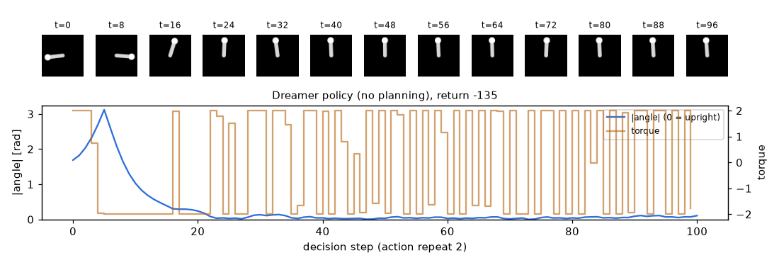
The trained actor swings the pendulum upright with a single network pass and no planning (starting about 1.7 rad from the top, return −135). The strategy is the same as PlaNet's: let it fall to build momentum (decisions 0 to 5), pull it up with maximum torque in the opposite direction (decisions 5 to 16), and balance at the top. The difference is the shape of the torque. Dreamer almost always outputs either \(+2\) or \(-2\) (bang-bang control). This is the same phenomenon as the entropy in the log dropping to around \(-7\): the pre-tanh values grew large and the actions stuck to \(\pm 1\). In a low-torque task like the pendulum, bang-bang control is a fairly good policy, so it does balance, but the pole jitters slightly at the top. PlaNet averages 100 elites, which yields smooth actions with small torques at the top.
Dreamer's World Model imagines the first few steps (t = 5 to 9) almost identically to reality, but starts falling behind around t = 12; while the real pendulum stands at the top, the imagined pendulum fails to reach the top and falls back to swing at the bottom. The distant future beyond the imagination horizon \(H = 15\) is left to the critic, and during real action the belief state is corrected with a new image at every moment, so this error does not ruin the policy. However, inaccurate imagination near the top makes it hard for the actor to learn fine balancing there, which is likely related to the bang-bang control and the jitter.
PlaNet vs. Dreamer
After training, both were evaluated on the same 10 unseen starting states.
| Policy | Mean return (10 episodes) | Standard deviation | Min / max | Time per decision |
| Random actions | −1194.5 | - | - | - |
| PlaNet (Chapter 11, CEM planning) | −196.8 | 113.7 | −376.2 / −0.5 | About 100 ms |
| Dreamer (actor) | −196.4 | 120.9 | −393.3 / −3.3 | About 5 ms |
Decision time includes one environment step, rendering, and the encoder, so the gap is even larger if only the planning itself is compared. In this experiment (21,000 environment steps), Dreamer matched PlaNet's performance with decisions about 20 times faster, while its training was bumpier. The Dreamer paper reports that on 20 DMC tasks Dreamer outperformed prior methods, including PlaNet, in data efficiency, computation time, and final performance. This task can be seen far enough ahead with a 12-step planning horizon, so the advantage of using a value function to look beyond the horizon is hard to show here.
| Item | Value |
| Total training time (laptop GPU, shared with PlaNet) | 4,806 s ≈ 80 minutes |
| Same GPU used alone ( | 2,575 s ≈ 43 minutes, about 1.5 ms per decision |
| One training step (CPU, 4 threads, \(B = 50\)) | About 23 s. The default settings (10,000 steps) are practically infeasible on CPU |
| Same, | About 5 s. Over half a day for 10,000 steps |
| | About 15 s (smoke test) |
Training time is similar to PlaNet's. Each training step is heavier because of imagination, the actor, and the critic, but data collection is faster by the same margin because there is no planning.
Experiment with return normalization
DreamerV3-style return normalization was enabled with --return-norm, with everything else unchanged (same seed). With the GPU to itself it took 2,575 seconds; the last line was imag G -16.20 critic 7.012 ent -7.95, and the final evaluation was mean −248.5, std 117.5, min −392.6, max −132.3.
| Setting | Final mean return (10 episodes) | Range of evaluation returns during training |
| Dreamer (default) | −196.4 ± 120.9 | −806 to −133 |
| Dreamer + return normalization | −248.5 ± 117.5 | −604 to −140 |
The result did not improve. Interpretation:
- A single-seed comparison is not conclusive. In both settings the evaluation return swings by hundreds during training, so a difference of about 50 in the mean can come from the seed alone. Five or more seeds with means and confidence intervals are needed.
- V3's techniques are a package. Return normalization was tuned together with an entropy coefficient of \(3\times10^{-4}\), symlog and two-hot critics, slow-critic regularization, and more, so detaching one piece and attaching it to V1 may not reproduce its effect.
- This task was already scaled with the reward scale. The benefit of return normalization is not having to tune each task by hand, but the reward scale of 0.1 already did that, so there is little left to gain.
DreamerV2: categorical latents and KL balancing
DreamerV1 did well on continuous control tasks (DMC) but was weak on tasks like Atari where scenes change abruptly. DreamerV2, from Hafner, Lillicrap, Norouzi, and Ba's Mastering Atari with Discrete World Models (ICLR 2021), was the first agent trained purely within a World Model to reach human-level performance across 55 Atari games.
Categorical latent variables
V1's \(z_t\) is a 30-dimensional Gaussian. V2 uses 32 categorical variables, each holding one of 32 classes as a one-hot vector. The result is a sparse vector with only 32 of its 32 × 32 = 1024 entries set to 1. The paper admits it does not know for sure why categoricals work better, and offers hypotheses:
- A single Gaussian has one mode, but a categorical can represent multimodal futures, such as "the enemy appears from the left / from the right."
- It suits discontinuous changes such as scene cuts and item pickups.
- It may optimize better (a conjecture that straight-through gradients may be easier to handle than reparameterization gradients).
Straight-through estimator
A categorical sample (one-hot) is a step function of the probabilities \(p\), so its derivative is zero or undefined and reparameterization cannot be used. V2 uses the straight-through estimator.
\(z = \operatorname{onehot} + p - \operatorname{sg}(p)\)
- Value: \(\operatorname{sg}(p)\) equals \(p\) in value, so \(z = \operatorname{onehot}\). In the forward pass, \(z\) is exactly the sampled one-hot vector.
- Gradient: the sampled one-hot is a constant not connected to the graph, and the derivative of \(\operatorname{sg}\) is 0, so \(\frac{\partial z}{\partial p} = 0 + I - 0 = I\), that is, \(\frac{\partial \mathcal{L}}{\partial p} = \frac{\partial \mathcal{L}}{\partial z}\). In the backward pass, the gradient arriving at \(z\) is passed straight to \(p\). Treating sampling as the identity function does not give the exact gradient (it is biased), but it works well in practice.
- Example: if the second class is drawn from \(p = (0.2,\ 0.7,\ 0.1)\), the forward value is \(z = (0, 1, 0)\), and in the backward pass \((g_1, g_2, g_3)\) flows to all three probabilities.
probs = logits.softmax(-1)                                   # (..., 32, 32)
idx = torch.distributions.Categorical(probs=probs).sample()  # (..., 32)
onehot = F.one_hot(idx, 32).float()
z = onehot + probs - probs.detach()                          # 값은 원-핫, 기울기는 probs 로
KL balancing
The KL term \(D_{\mathrm{KL}}(q \,\Vert\, p)\) in the sequential ELBO pulls the posterior \(q\) and the prior \(p\) toward each other. If both move at the same rate, the posterior gets pulled toward the poor prior of early training and carries less information from the images. What we want is for the prior to follow the posterior (that is, to learn the dynamics). KL balancing adjusts this ratio using stop-gradients.
\(\mathcal{L}_{\text{KL}} = \alpha\,D_{\mathrm{KL}}\big(\operatorname{sg}(q)\ \Vert\ p\big) + (1 - \alpha)\,D_{\mathrm{KL}}\big(q\ \Vert\ \operatorname{sg}(p)\big),\qquad \alpha = 0.8\)
- Value: \(\operatorname{sg}\) does not change values and the weights sum to 1, so the loss value equals the original KL.
- The gradient to the prior comes only from the first term: \(\alpha\,\nabla D_{\mathrm{KL}}(q \,\Vert\, p)\).
- The gradient to the posterior comes only from the second term: \((1-\alpha)\,\nabla D_{\mathrm{KL}}(q \,\Vert\, p)\).
- With \(\alpha = 0.8\), the prior receives 80% of the KL gradient and the posterior only 20%. The value stays the same; the mechanism only decides who moves more.
Discrete actions and REINFORCE
Atari actions are discrete, so reparameterization gradients with respect to actions are unavailable. On Atari, V2 applies REINFORCE to the imagined trajectories.
\(\mathcal{L}(\psi) = -\sum_{t}\Big[\rho\,\log\pi_\psi(a_t \mid s_t)\,\operatorname{sg}\big(V^\lambda_t - v_\xi(s_t)\big) + (1-\rho)\,V^\lambda_t + \eta\,\mathcal{H}[\pi_\psi(\cdot \mid s_t)]\Big]\)
\(\rho\) is the mixing ratio between the two estimators. The paper used \(\rho = 1\) (REINFORCE only) on Atari and \(\rho = 0\) (dynamics backpropagation only) on continuous control. \(V^\lambda_t - v_\xi(s_t)\) is the advantage. Subtracting a baseline \(b\) that does not depend on the action (here \(v_\xi(s_t)\)) leaves the expected gradient unchanged.
\(\mathbb{E}_{a \sim \pi}\big[b\,\nabla_\psi \log\pi_\psi(a \mid s)\big] = b\sum_{a}\pi_\psi(a \mid s)\,\frac{\nabla_\psi\pi_\psi(a \mid s)}{\pi_\psi(a \mid s)} = b\,\nabla_\psi\sum_{a}\pi_\psi(a \mid s) = b\,\nabla_\psi\, 1 = 0\)
The baseline shifts the returns toward 0 without changing the expectation, which reduces variance. V2 also added a slow target critic (used in this implementation), layer normalization, and other changes.
DreamerV3: one configuration across many domains
Reinforcement learning algorithms usually need their hyperparameters retuned for each task (this chapter's reward scale of 0.1 is one example). DreamerV3 by Hafner, Pasukonis, Ba, and Lillicrap (Mastering diverse control tasks through world models, released on arXiv in 2023, published in Nature in 2025) performed well on more than 150 tasks, including Atari, DMC, and Minecraft, with a single fixed configuration, and became the first algorithm to mine diamonds in Minecraft from scratch without human data or curricula. The core is a set of techniques that make it robust to the magnitude of signals.
symlog and symexp
The magnitude of rewards and observations varies widely across tasks (the pendulum's is \(-16\) to \(0\); some games reach thousands). Fitting large numbers with squared error makes gradients explode, while small numbers get drowned out. V3 trains on targets squashed with symlog (symmetric logarithm) and maps predictions back with symexp.
\(\operatorname{symlog}(x) = \operatorname{sign}(x)\,\log\big(\vert x\vert + 1\big),\qquad \operatorname{symexp}(x) = \operatorname{sign}(x)\big(\exp(\vert x\vert) - 1\big)\)
- Inverse: if \(y = \operatorname{symlog}(x)\), then since \(\log(\vert x\vert+1) \ge 0\), \(\operatorname{sign}(y) = \operatorname{sign}(x)\) and \(\vert y\vert = \log(\vert x\vert + 1)\), so \(\operatorname{symexp}(y) = \operatorname{sign}(x)\big(\exp(\log(\vert x\vert+1)) - 1\big) = x\).
- Derivative: differentiating each side separately and combining gives \(\frac{d}{dx}\operatorname{symlog}(x) = \frac{1}{\vert x\vert + 1}\). It is 1 at \(x = 0\) (small values pass almost unchanged) and shrinks as \(\vert x\vert\) grows, compressing large values.
- Example: \(\operatorname{symlog}(10) = \log 11 \approx 2.398\), \(\operatorname{symlog}(1000) = \log 1001 \approx 6.909\), \(\operatorname{symlog}(-10) \approx -2.398\). The ratio between 1000 and 10 shrinks from 100× to about 2.9×.
Unlike the ordinary logarithm, it is defined at 0 and for negative numbers, and its slope near the origin is 1, so it does not distort small values. V3 applies this transform to vector observation inputs and reconstruction targets, and to reward and value predictions.
two-hot encoding
V3 turns reward and value regression into a classification problem. Evenly spaced bins \(b_1 \lt b_2 \lt \cdots \lt b_K\) are laid out in symlog space (255 bins from \(-20\) to \(20\) in the first arXiv version), and the network outputs softmax probabilities \(p_1, \dots, p_K\) over the bins. The target \(y\) is split between the two neighboring bins that bracket it (two-hot encoding). For \(b_k \le y \lt b_{k+1}\) there are two conditions:
\(w_k + w_{k+1} = 1,\qquad w_k\, b_k + w_{k+1}\, b_{k+1} = y\)
Substituting \(w_k = 1 - w_{k+1}\) and solving gives linear interpolation. All other bins get weight 0.
\(w_{k+1} = \frac{y - b_k}{b_{k+1} - b_k},\qquad w_k = \frac{b_{k+1} - y}{b_{k+1} - b_k}\)
Example: a reward of \(r = 10\) gives \(y = \operatorname{symlog}(10) \approx 2.398\). With bin spacing 1, \(b_k = 2\), and \(b_{k+1} = 3\), we get \(w_k = 0.602\) and \(w_{k+1} = 0.398\), and \(0.602 \times 2 + 0.398 \times 3 = 2.398\) recovers the value.
The loss is the cross entropy \(-\sum_i w_i \log p_i\) between the target weights and the predicted probabilities, and the prediction is \(\hat{y} = \operatorname{symexp}\big(\sum_i p_i\, b_i\big)\). The cross-entropy gradient has the form \(p - w\) and its magnitude is always at most 1, so whether the target is 1 or 10,000, the gradient's magnitude is independent of the target's. That is why regression is turned into classification. Everything up to this point follows the first arXiv version. The 2024 revision instead lays out the bins exponentially as \(b = \operatorname{symexp}(-20, \dots, 20)\), converts the raw target directly to two-hot, and reads the prediction as \(\hat{y} = \sum_i p_i\, b_i\) (symexp moved from outside the mean to inside it).
Free bits and splitting the KL
V3 uses Chapter 11's free nats at 1 nat (the paper calls it "free bits") and splits V2's KL balancing into two losses, applying it to each.
\(\mathcal{L}_{\text{dyn}} = \max\Big(1,\ D_{\mathrm{KL}}\big(\operatorname{sg}(q)\ \Vert\ p\big)\Big),\qquad \mathcal{L}_{\text{rep}} = \max\Big(1,\ D_{\mathrm{KL}}\big(q\ \Vert\ \operatorname{sg}(p)\big)\Big)\)
\(\mathcal{L} = \mathcal{L}_{\text{pred}} + \beta_{\text{dyn}}\,\mathcal{L}_{\text{dyn}} + \beta_{\text{rep}}\,\mathcal{L}_{\text{rep}}\)
\(\mathcal{L}_{\text{dyn}}\) trains the prior (dynamics) and \(\mathcal{L}_{\text{rep}}\) trains the posterior (representation). \(\mathcal{L}_{\text{pred}}\) is the loss for predicting reconstruction, reward, and continuation (whether the episode ends). The weights differ between versions: the first arXiv version (January 2023) uses \(\beta_{\text{dyn}} = 0.5\), \(\beta_{\text{rep}} = 0.1\), and the revision (2024) uses \(\beta_{\text{dyn}} = 1\), \(\beta_{\text{rep}} = 0.1\). Either way the prior's weight is much larger, playing the same role as V2's \(\alpha = 0.8\) (first version \(0.5/0.6 \approx 0.83\), revision \(1/1.1 \approx 0.91\)). When the KL falls below 1 nat, the gradient of that term switches off, just as derived in Chapter 11.
unimix
If the probability of some class in a categorical distribution approaches 0, the \(\log(q/p)\) in the KL can blow up. V3 mixes 1% of a uniform distribution into the network's probabilities.
\(p_i = 0.99\cdot\operatorname{softmax}(\ell)_i + 0.01\cdot\frac{1}{K}\)
Every class has probability at least \(0.01/K\), so for any \(q_i \le 1\), \(\log(q_i/p_i) \le \log(100K)\) is bounded above. With \(K = 32\) this is \(\log 3200 \approx 8.07\). The same technique is used for policies over discrete actions.
Return normalization
The magnitude of the actor's gradient is proportional to the magnitude of the returns. In tasks with large rewards the actor gradient overwhelms the entropy bonus (too little exploration), and in tasks with small rewards the opposite happens. V3 divides the returns by their spread.
\(S = \operatorname{EMA}\Big(\operatorname{Per}(V^\lambda, 95) - \operatorname{Per}(V^\lambda, 5),\ 0.99\Big),\qquad \frac{V^\lambda_t - v_\xi(s_t)}{\max(1,\ S)}\)
- \(\operatorname{Per}(\cdot, 95)\) is the 95th percentile of the returns in the batch. Using percentiles instead of the max and min keeps it robust to outliers.
- An EMA (exponential moving average, coefficient 0.99) tracks the value without fluctuating from batch to batch: \(S \leftarrow 0.99\,S + 0.01\,(\text{range})\).
- \(\max(1, S)\) prevents amplifying small return differences (noise) in sparse-reward tasks. Returns are scaled down only when the spread exceeds 1.
- The entropy coefficient is fixed at \(\eta = 3 \times 10^{-4}\) for all tasks. This is possible because the magnitude of returns has been normalized.
Using REINFORCE on the advantage with the critic value subtracted, as in the formula above, is the form from the 2024 revision (for both discrete and continuous actions). The first arXiv version used \(\operatorname{sg}(V^\lambda_t)/\max(1, S)\) and, like V2, used dynamics backpropagation for continuous actions and REINFORCE for discrete ones. This chapter's code adds it as the --return-norm option (if cfg.return_norm: in train_step); since it uses dynamics backpropagation, it divides the returns directly without subtracting \(v_\xi(s_t)\), as in the first version.
Comparing the three versions
| DreamerV1 (2020) | DreamerV2 (2021) | DreamerV3 (2023, 2025) | |
| Latent \(z\) | 30-dim Gaussian | Categorical 32 × 32 (straight-through) | Categorical + 1% unimix |
| KL | Free nats 3 | KL balancing \(\alpha = 0.8\) | dyn 0.5 (revision: 1) / rep 0.1, free bits 1 |
| Reward, value | Gaussian regression | Gaussian regression | symlog + two-hot classification |
| Actor gradient | Dynamics backpropagation | Atari: REINFORCE / continuous: backpropagation | Normalized returns (first version), advantage + REINFORCE (revision) |
| Critic target | λ-return | λ-return + slow critic | λ-return + slow critic (EMA) |
| Headline result | 20 DMC tasks | 55 Atari games, human level | 150+ tasks with a fixed configuration, Minecraft diamonds |
Common problems
| Symptom | Common cause | Things to try |
| Imagined return ( | The actor exploits errors in the World Model (model exploitation). | Collect more data. Keep exploration noise and entropy. Check the model by comparing imagined and real frames. |
| Critic loss keeps growing | Values are too large in magnitude, or the target is unstable. | Reward scale, slow critic, (V3) return normalization and two-hot. |
| The actor always outputs \(\pm 1\) | \(\tanh\) saturation. For the pendulum, this bang-bang control is a fairly good policy. | Increase the entropy coefficient only if it causes problems. |
| Early returns are worse than random | The model is still poor, so the best action in imagination is bad in reality. | This is normal and improves as data accumulates. Increasing the number of seed episodes also helps. |
| NaN | \(a = \pm 1\) in \(\log(1 - a^2)\), or a standard deviation of 0. | Add a small constant (\(10^{-6}\)), a minimum standard deviation, and gradient clipping. |
Summary
- PlaNet's planning is expensive (120,000 steps per decision) and short-sighted. Dreamer trains an actor and a critic in imagination and acts with a single network pass at decision time.
- Imagination starts from the 2,500 posterior states obtained during World Model training and rolls forward \(H = 15\) steps with the actor and the RSSM prior.
- The λ-return is a weighted average of n-step returns (weights sum to 1), computed with the recursion \(V^\lambda_t = \hat{r}_t + \gamma[(1-\lambda)v(s_{t+1}) + \lambda V^\lambda_{t+1}]\), \(V^\lambda_H = v(s_H)\).
- The critic regresses onto \(\operatorname{sg}(V^\lambda_t)\), and the actor increases the λ-return by differentiating through the World Model (reparameterization gradients). The model is frozen (
requires_grad_(False)), not detached. - By the change-of-variables formula, the entropy of a tanh-Gaussian policy is \(\mathcal{H}[u] + \mathbb{E}[\log(1 - a^2)]\).
- In the pendulum experiment, Dreamer matched PlaNet's mean return (−196.4 vs. −196.8) with decisions about 20 times faster (about 5 ms vs. about 100 ms), while its learning curve fluctuated more.
- V2 added categorical latents with the straight-through estimator (\(z = \operatorname{onehot} + p - \operatorname{sg}(p)\)), KL balancing (\(\alpha = 0.8\)), and REINFORCE for discrete actions. V3 used symlog, two-hot, free bits of 1, 1% unimix, and return normalization so that a single configuration works across many domains.
Review questions
- 1. With \(\gamma = 1\), what is \(V^\lambda_0\) of an \(H = 2\) imagined trajectory for \(\lambda = 0\) and for \(\lambda = 1\)?
- \(\lambda = 0\): \(V^\lambda_0 = \hat{r}_0 + v(s_1)\) (the one-step TD target; \(v(s_2)\) and \(\hat{r}_1\) are not used). \(\lambda = 1\): \(V^\lambda_1 = \hat{r}_1 + v(s_2)\) and \(V^\lambda_0 = \hat{r}_0 + \hat{r}_1 + v(s_2)\) (the 2-step return using imagination all the way to the end).
- 2. What happens if, instead of freezing the World Model during actor learning, the imagined states are cut with
.detach()? - The path from action \(a_t\) to the next state \(s_{t+1}\) is cut, so the gradient no longer reflects how the λ-return depends on the actions. Apart from the entropy term, no gradient reaches the actor, so it cannot learn to increase the return. Freezing means "do not update, but let gradients through"; detaching means "do not let them through."
- 3. What is the entropy of a 1-D Gaussian \(u\) with mean 0 and \(\sigma = 0.5\), and of \(a = \tanh(u)\)?
- \(\mathcal{H}[u] = \frac{1}{2}\log(2\pi e) + \log 0.5 \approx 1.419 - 0.693 = 0.726\). When \(u\) is near 0, \(\log(1 - a^2) \approx -u^2\), so the correction term is roughly \(-\sigma^2 = -0.25\) (a Monte Carlo estimate with 2 million samples gives \(-0.23\)). Hence \(\mathcal{H}[a] \approx 0.50\). With \(\sigma = 0.1\) the correction nearly vanishes at about \(-0.01\), while if \(u\) concentrates near \(\pm 3\), \(1 - \tanh^2(3) \approx 0.0099\) makes the log about \(-4.6\) and the entropy drops sharply.
- 4. With bins \(b = (-1, 0, 1, 2)\), what is the two-hot vector for \(y = 1.25\)?
- \(b_k = 1\) and \(b_{k+1} = 2\), so \(w_{k+1} = 0.25\) and \(w_k = 0.75\), giving the vector \((0, 0, 0.75, 0.25)\). Check: \(0.75 \times 1 + 0.25 \times 2 = 1.25\).
- 5. In KL balancing, what do \(\alpha = 0.5\) and \(\alpha = 1\) mean?
- With \(\alpha = 0.5\), the prior and the posterior receive gradients in equal proportion. The value is the original KL and both gradients are scaled by 0.5, which is the same as training with \(0.5\,D_{\mathrm{KL}}(q \,\Vert\, p)\) (the 0.5 is absorbed into the learning rate). With \(\alpha = 1\), the second term disappears, so the posterior receives no gradient from the KL and is trained only by the reconstruction loss.
See also
- World Models:Tutorial
- World Models
- World Models:Tutorial:05 Reinforcement learning basics
- World Models:Tutorial:11 RSSM and PlaNet
- Reinforcement learning
- Policy
- Backpropagation through time
- Entropy
- Cross entropy