WorldModels:Tutorial:11-RSSM-PlaNet
lastmod 2026-11-18created 2026-11-172 edits
RSSM and PlaNet is chapter 11 of the World Model tutorial. It merges the eyes (VAE) and the memory (MDN-RNN), which were trained separately in chapter 10, into a single model trained end to end, the RSSM (Recurrent State-Space Model). It then uses PlaNet, which plans actions inside that model's imagination, to swing a pendulum upright from 64×64 images alone. The core of the chapter is the derivation of the sequential ELBO, the RSSM's training objective, and the RSSM built here serves unchanged as the backbone of the Dreamer family in chapter 12.
- Original: 11. RSSM and PlaNet
- Practice code:
code/ch11_rssm_planet.py,code/wm_envs.py(the main settings take about 76 minutes on a laptop GPU;--quicktakes about 1 minute on CPU) - Previous: 10. World Models by Ha and Schmidhuber / Next: 12. Dreamer
Background: limitations of World Models and partial observability
Chapters 6 and 7 received the pendulum state exactly, as three numbers \([\cos\theta, \sin\theta, \dot\theta]\). From chapter 8 on, the agent sees only 64×64 images. The World Models approach of chapter 10 handled this with V (VAE, trained on each image independently), M (MDN-RNN, trained separately after V is fully trained), and C (a controller trained with CMA-ES), but it leaves three shortcomings.
- V does not know what matters. Its only objective is to "reconstruct the image well", so there is no guarantee that it captures the information needed to predict the future or judge rewards.
- Training is split into two stages. M cannot change the \(z\) that V has already fixed, so the two cannot jointly search for a representation that is good for prediction.
- There is no planning. C picks actions reflexively at every moment.
Hafner et al.'s Learning Latent Dynamics for Planning from Pixels (ICML 2019) introduced PlaNet (Deep Planning Network), which addresses all of these problems at once. Its key component is the RSSM.
A single image cannot reveal velocity
A single image \(o_t\) reveals only the angle \(\theta\). For the same image, if \(\dot\theta = +3\) rad/s (clockwise) the bar moves down to the right in the next instant, and if \(\dot\theta = -3\) rad/s (counterclockwise) it moves up. A pendulum observed through images is a partially observable Markov decision process (POMDP), and the observation \(o_t\) alone does not satisfy the Markov property (Markov decision process). The solution is to carry a belief state that summarizes everything seen so far. For a pendulum, remembering the change in angle over the last two or three frames is enough to estimate velocity. The RSSM learns this belief state with a neural network.
Latent state-space models
A state-space model (SSM) assumes a hidden state \(s_t\) that cannot be observed directly and changes over time, and that only the observations \(o_t\) it produces are visible. The Kalman filter is a typical example.
\(\begin{align} \text{Transition} &: \quad s_t \sim p(s_t \mid s_{t-1}, a_{t-1}) \\ \text{Observation} &: \quad o_t \sim p(o_t \mid s_t) \\ \text{Reward} &: \quad r_t \sim p(r_t \mid s_t) \end{align}\)
In a Kalman filter these distributions are linear equations written by hand, but in a latent state-space model even the meaning of the state \(s_t\) is left undefined, and the neural network builds it on its own.
Indexing convention for rewards and actions
Chapter 5 wrote the reward received for taking action \(a_t\) in state \(s_t\) as \(r_t\). Following the PlaNet and Dreamer papers, this chapter writes the reward received on arriving at state \(s_t\) (the result of the previous action \(a_{t-1}\)) as \(r_t\) and predicts it from \(s_t\). In chapter 5 notation this is \(r_{t-1}\). \(a_{t-1}\) is the action that moves from \(s_{t-1}\) to \(s_t\).
| Time | Image | Action just before this image | Reward received on arriving at this image |
| \(t = 0\) | \(o_0\) (first image) | None (filled with 0) | None (excluded from training) |
| \(t = 1\) | \(o_1\) | \(a_0\) | \(r_1\) |
| \(t = 2\) | \(o_2\) | \(a_1\) | \(r_2\) |
The replay buffer also stores obs[t], prev_action[t], reward[t], and first[t] following this table. Each slot at time \(t\) holds everything needed at that time, which keeps the code simple.
Filtering
Estimating the current state from the images seen so far, \(o_{1:t}\), and the actions taken, \(a_{0:t-1}\), that is, computing \(p(s_t \mid o_{1:t}, a_{0:t-1})\), is called filtering. The true distribution is defined by Bayes' theorem, but the integral is intractable for a neural network model. So, as in a VAE, it is approximated with an inference network \(q\); this is the posterior model introduced below.
Three designs: deterministic RNN, stochastic SSM, RSSM
- Attempt 1 (deterministic RNN only)
- Compute the hidden state as \(h_t = f(h_{t-1}, a_{t-1}, o_{t-1})\) and predict the next image from \(h_t\). During training, real images keep coming in and it works well, but problems arise during planning. A deterministic model produces only one future for a given input, so when the future can branch (will the bar fall to the left or to the right from the top?), it minimizes squared error by predicting the average of the branches: a blurry future that never actually happens. Also, it always receives images during training but is rolled out without images only during planning, so the training and usage conditions do not match.
- Attempt 2 (stochastic state only)
- Sample from a distribution at every step, as in \(s_t \sim p(s_t \mid s_{t-1}, a_{t-1})\). This can represent branching futures and can be trained with the ELBO. However, all information has to pass through a sampling step at every step to reach the next one, which makes it hard to carry information accurately across many steps (as in a game of telephone, noise creeps in every time).
- Solution (RSSM)
- Split the state into two parts. The deterministic state \(h_t\) is a deterministic vector computed by a GRU; it serves as memory, carrying information over long spans without noise. The stochastic state \(z_t\) is a vector sampled from a Gaussian at every step; it represents uncertainty, covering what is not yet known and branching futures. The model state is \(s_t = (h_t, z_t)\).
| Approach | Long-term memory | Branching futures | Trainable with ELBO |
| (a) Deterministic RNN | Good | Poor (predicts the average) | No (no latent variable) |
| (b) Stochastic SSM | Weak (noise at every step) | Good | Yes |
| (c) RSSM | Good (\(h\)) | Good (\(z\)) | Yes |
The original tutorial uses this analogy: a driver going through a tunnel remembers the speed and direction from before entering (\(h\)) and imagines the car's position, but the exact position is uncertain (\(z\)); on leaving the tunnel and seeing the scenery (\(o_t\)), the driver corrects the position estimate. The imagined position inside the tunnel is the prior, and the position corrected after seeing the scenery is the posterior.
The five components of the RSSM
| Component | Equation | Role | Code |
| ① Deterministic state model | \(h_t = f_\theta(h_{t-1}, z_{t-1}, a_{t-1})\) | Moves memory one step forward (GRU) | First part of |
| ② Prior (transition) model | \(p_\theta(z_t \mid h_t)\) | Predicts \(z_t\) before seeing the image | |
| ③ Posterior (representation) model | \(q_\phi(z_t \mid h_t, o_t)\) | Corrects \(z_t\) after seeing the image | |
| ④ Observation model (decoder) | \(p_\theta(o_t \mid h_t, z_t)\) | Redraws the image from the state | |
| ⑤ Reward model | \(p_\theta(r_t \mid h_t, z_t)\) | Predicts the reward from the state | |
Unrolled over time, the structure looks like this.
- \(h_{t-1}\), \(z_{t-1}\), and \(a_{t-1}\) go into the GRU and become \(h_t\).
- The prior \(p(z_t \mid h_t)\) comes from \(h_t\).
- The observation and reward decoders produce \(o_t\) and \(r_t\) from the full state \((h_t, z_t)\).
- The only inference path is the posterior \(q(z_t \mid h_t, o_t)\), which corrects \(z_t\) after seeing the image \(o_t\). The generative model has no \(o \to z\) arrow.
①, ②, ④, and ⑤ form the generative model, which can be computed without images; only ③ looks at images. After training, repeating just ① → ② lets the model imagine the future without images. This is the "dream" of a World Model.
Shape of the distributions: diagonal Gaussians
Both the prior and the posterior are diagonal Gaussians, independent in each dimension (Normal distribution).
\(p_\theta(z_t \mid h_t) = \mathcal{N}\big(z_t;\ \mu_\theta(h_t),\ \operatorname{diag}(\sigma_\theta(h_t)^2)\big)\)
\(q_\phi(z_t \mid h_t, o_t) = \mathcal{N}\big(z_t;\ \mu_\phi(h_t, e_t),\ \operatorname{diag}(\sigma_\phi(h_t, e_t)^2)\big)\)
\(e_t = \mathrm{enc}_\phi(o_t)\) is the feature vector (1024 numbers) that the convolutional encoder extracts from the image. The standard deviation is obtained by passing the network output \(x\) through softplus and adding a minimum value (F.softplus(std) + self.min_std).
\(\sigma = \operatorname{softplus}(x) + \sigma_{\min} = \log(1 + e^{x}) + 0.1\)
- Since \(e^x \gt 0\), we have \(\log(1 + e^x) \gt \log 1 = 0\), so \(\sigma \gt 0.1\) for any \(x\). \(\sigma_{\min} = 0.1\) is a floor that keeps the distribution from shrinking to a single point.
- By the chain rule, the derivative is \(\frac{d}{dx}\log(1 + e^{x}) = \frac{e^{x}}{1 + e^{x}} = \frac{1}{1 + e^{-x}} = \operatorname{sigmoid}(x)\). The gradient always stays alive between 0 and 1, which keeps training stable.
- Example: when \(x = 0\), \(\sigma = \log 2 + 0.1 \approx 0.793\) and the gradient is 0.5.
Deterministic state model: GRU
\([z_{t-1}, a_{t-1}]\) is turned into a 200-dimensional input \(x_t\) by a linear layer and an ELU activation, and the GRU mixes it with the previous memory \(h_{t-1}\). ELU is \(x\) when \(x \gt 0\) and \(e^x - 1\) when \(x \le 0\). The negative side approaches \(-1\) smoothly, and the gradient \(e^x\) only shrinks; it never becomes exactly 0 as in ReLU. nn.GRUCell computes the following (\(\odot\) is element-wise multiplication).
\(\begin{align} \rho_t &= \operatorname{sigmoid}(W_\rho x_t + U_\rho h_{t-1} + b_\rho) && \text{(reset gate: how much of the old memory to look at)} \\ u_t &= \operatorname{sigmoid}(W_u x_t + U_u h_{t-1} + b_u) && \text{(update gate: how much of the old memory to keep)} \\ n_t &= \tanh\big(W_n x_t + b_n + \rho_t \odot (U_n h_{t-1} + b'_n)\big) && \text{(new candidate memory)} \\ h_t &= (1 - u_t) \odot n_t + u_t \odot h_{t-1} && \text{(mix the old memory and the new candidate)} \end{align}\)
The structure is the same as in chapter 9; only the notation differs. Since \(r\) is used for rewards, the reset gate is written \(\rho_t\), and the candidate \(\tilde h_t\) is written \(n_t\) after the PyTorch name. The reset gate is not applied to \(h_{t-1}\) first; it multiplies \(U_n h_{t-1} + b'_n\) after that term is computed. In the last line, entries where \(u_t\) is close to 1 pass the old memory through almost unchanged, so information crosses many steps without noise. This path is why the RSSM avoids the weakness of the stochastic SSM.
Code: RSSM
mlp(입력, 너비, 출력, layers=n) (input size, hidden width, output size) is a helper function that stacks (linear layer → ELU) n times and adds one more linear layer at the end.
class RSSM(nn.Module):
    """순환 상태 공간 모델 (Recurrent State-Space Model).

    결정 경로   h_t = f(h_{t-1}, z_{t-1}, a_{t-1})      ← GRU
    사전(prior) p(z_t | h_t)        = N(μ, σ²)        ← 그림을 보기 전의 예측
    사후(post)  q(z_t | h_t, e_t)   = N(μ', σ'²)      ← 그림 특징 e_t 까지 본 추측
    """

    def __init__(self, act_dim: int, embed_dim: int, deter=200, stoch=30, hidden=200, min_std=0.1):
        super().__init__()
        self.deter, self.stoch, self.min_std = deter, stoch, min_std
        self.inp = nn.Linear(stoch + act_dim, hidden)  # [z_{t-1}, a_{t-1}] → GRU 입력
        self.gru = nn.GRUCell(hidden, deter)
        self.prior_net = mlp(deter, hidden, 2 * stoch, layers=1)
        self.post_net = mlp(deter + embed_dim, hidden, 2 * stoch, layers=1)

    def initial(self, batch: int, device) -> tuple[torch.Tensor, torch.Tensor]:
        return torch.zeros(batch, self.deter, device=device), torch.zeros(batch, self.stoch, device=device)

    def _dist(self, x: torch.Tensor):
        mean, std = x.chunk(2, dim=-1)
        std = F.softplus(std) + self.min_std  # 표준편차는 늘 양수, 그리고 min_std 이상
        return mean, std

    def img_step(self, h, z, action, sample: bool = True):
        """그림 없이 한 스텝 상상한다: (h_{t-1}, z_{t-1}, a_{t-1}) → h_t, z_t ~ p(z_t | h_t)."""
        x = F.elu(self.inp(torch.cat([z, action], -1)))
        h = self.gru(x, h)
        mean, std = self._dist(self.prior_net(h))
        z = mean + std * torch.randn_like(std) if sample else mean  # 재매개변수화
        return h, z, mean, std

    def obs_step(self, h, z, action, embed):
        """그림을 보며 한 스텝: 사전으로 h_t 를 만든 뒤, 그림 특징 e_t 로 z_t 를 고쳐 잡는다."""
        h, _, prior_mean, prior_std = self.img_step(h, z, action)
        post_mean, post_std = self._dist(self.post_net(torch.cat([h, embed], -1)))
        z = post_mean + post_std * torch.randn_like(post_std)
        return h, z, (prior_mean, prior_std), (post_mean, post_std)

    def observe(self, embeds, prev_actions, h=None, z=None):
        """시퀀스 전체를 시간 순서대로 펼친다. embeds (B, L, E), prev_actions (B, L, A)."""
        B, L = embeds.shape[:2]
        if h is None:
            h, z = self.initial(B, embeds.device)
        out = {k: [] for k in ("h", "z", "prior_mean", "prior_std", "post_mean", "post_std")}
        for t in range(L):
            h, z, (pm, ps), (qm, qs) = self.obs_step(h, z, prev_actions[:, t], embeds[:, t])
            for k, v in zip(out, (h, z, pm, ps, qm, qs)):
                out[k].append(v)
        return {k: torch.stack(v, dim=1) for k, v in out.items()}  # 모두 (B, L, ·)
-
img_step: one step with eyes closed. It builds \(h_t\) with the GRU and samples \(z_t\) from the prior.mean + std * torch.randn_like(std)is the reparameterization trick from chapter 8: it turns sampling into a computation that multiplies fixed noise \(\epsilon \sim \mathcal{N}(0, I)\) by the standard deviation and adds the mean, so that gradients flow to \(\mu\) and \(\sigma\). This property becomes crucial in chapter 12. -
obs_step: one step with eyes open. It builds \(h_t\) and the prior withimg_step, then appends the image feature \(e_t\) to the same \(h_t\) to build the posterior and samples \(z_t\) from it. What is passed on to the next step is the \(z_t\) sampled from the posterior. -
observe: appliesobs_stepto the whole sequence. Because \(h_t\) depends on \(h_{t-1}\), the time axis must be processed in order.
Deriving the sequential ELBO
All components of the RSSM are trained together toward a single objective: maximum likelihood, which increases the log probability of the entire sequence of images and rewards (Maximum likelihood estimation).
\(\max_{\theta,\phi}\ \log p_\theta(o_{1:T},\ r_{1:T} \mid a_{0:T-1})\)
This probability cannot be computed directly, so a lower bound (the ELBO) is maximized instead. The derivation proceeds in four steps: (1) factorizing the joint distribution, (2) marginalization, (3) multiplying and dividing by \(q\) and applying Jensen's inequality, and (4) splitting the expectation over time. Below, the actions \(a_{0:T-1}\) are always given, so they are omitted from the conditioning. \(h_t\) is a value the GRU computes from \(z_{1:t-1}\) and the actions, and the only random variables are \(z_{1:T}\). \(h_0\) and \(z_0\) are zero vectors. The equations write the sum from \(t = 1\), but the code also treats the first image \(o_0\) as "one step starting from previous action 0 and \(h = z = 0\)" and includes it in the reconstruction and KL terms (only the reward term excludes \(t = 0\)).
Step 1: factorizing the joint distribution
Using the chain rule of probability, lay out the three variables at time \(t\), \((z_t, o_t, r_t)\), as one block, then apply the rule once more within the block ("past" means \(z_{1:t-1}, o_{1:t-1}, r_{1:t-1}\)).
\(p(o_{1:T}, r_{1:T}, z_{1:T}) = \prod_{t=1}^{T} p(z_t, o_t, r_t \mid z_{1:t-1}, o_{1:t-1}, r_{1:t-1})\)
\(p(z_t, o_t, r_t \mid \text{past}) = p(z_t \mid \text{past})\; p(o_t \mid z_t, \text{past})\; p(r_t \mid o_t, z_t, \text{past})\)
Now add two model assumptions.
- Assumption ①: \(p(z_t \mid \text{past}) = p(z_t \mid h_t)\). \(z_t\) depends on the past only through \(h_t\). Past \(o\) and \(r\) are merely outcomes generated from \(z\) in the generative model and do not directly affect \(z_t\).
- Assumption ②: \(p(o_t \mid z_t, \text{past}) = p(o_t \mid h_t, z_t)\), \(p(r_t \mid o_t, z_t, \text{past}) = p(r_t \mid h_t, z_t)\). Images and rewards are generated from the current state \(s_t = (h_t, z_t)\) alone. This also includes the assumption that \(r_t\) does not depend directly on \(o_t\).
\(p(o_{1:T}, r_{1:T}, z_{1:T}) = \prod_{t=1}^{T} p(z_t \mid h_t)\; p(o_t \mid h_t, z_t)\; p(r_t \mid h_t, z_t), \qquad h_t = f(h_{t-1}, z_{t-1}, a_{t-1})\)
The joint distribution is a product over time of prior × observation × reward, and these three components are prior_net, Decoder, and reward in the code. The inference model \(q\) is not derived but designed: it is defined as a per-step product in filtering form that does not look at future images. Here \(h_t\) is computed from \(z_{1:t-1}\) sampled from the posterior.
\(q(z_{1:T} \mid o_{1:T}) = \prod_{t=1}^{T} q(z_t \mid h_t, o_t)\)
Steps 2 and 3: marginalization and Jensen's inequality
\(\begin{align} \log p(o_{1:T}, r_{1:T}) &= \log \int p(o_{1:T}, r_{1:T}, z_{1:T})\, dz_{1:T} \\ &= \log \int q(z_{1:T} \mid o_{1:T})\, \frac{p(o_{1:T}, r_{1:T}, z_{1:T})}{q(z_{1:T} \mid o_{1:T})}\, dz_{1:T} \\ &= \log \mathbb{E}_{q}\left[ \frac{p(o_{1:T}, r_{1:T}, z_{1:T})}{q(z_{1:T} \mid o_{1:T})} \right] \\ &\ge \mathbb{E}_{q}\left[ \log \frac{p(o_{1:T}, r_{1:T}, z_{1:T})}{q(z_{1:T} \mid o_{1:T})} \right] \\ &= \mathbb{E}_{q}\left[ \sum_{t=1}^{T} \Big( \log p(o_t \mid h_t, z_t) + \log p(r_t \mid h_t, z_t) + \log p(z_t \mid h_t) - \log q(z_t \mid h_t, o_t) \Big) \right] \\ &= \sum_{t=1}^{T} \Big( \mathbb{E}_{q}[\log p(o_t \mid h_t, z_t)] + \mathbb{E}_{q}[\log p(r_t \mid h_t, z_t)] + \mathbb{E}_{q}[\log p(z_t \mid h_t) - \log q(z_t \mid h_t, o_t)] \Big) \end{align}\)
- The first line is marginalization. The integral is over 30 dimensions × \(T\) steps and cannot be computed directly.
- The second line multiplies by \(q/q = 1\) (\(q\) is Gaussian, so it is positive everywhere).
- The third line is the definition of expectation, \(\int q(z)\, g(z)\, dz = \mathbb{E}_{z \sim q}[g(z)]\).
- The fourth line is Jensen's inequality. Since \(\log\) is concave, \(\log \mathbb{E}[X] \ge \mathbb{E}[\log X]\); this is where the inequality first appears.
- The fifth line substitutes the factorization and the definition of \(q\), turning the log of a product into a sum and the log of a quotient into a difference.
- The sixth line is linearity of expectation.
Step 4: splitting the expectation over time to form the KL
The term at time \(t\) depends only on \(z_{1:t}\). Unused future variables drop out of the expectation, because splitting \(q(z_{1:T}) = q(z_{1:t})\, q(z_{t+1:T} \mid z_{1:t})\) makes the inner integral equal to 1.
\(\mathbb{E}_{q(z_{1:T})}[g(z_{1:t})] = \int q(z_{1:t})\, g(z_{1:t}) \left[ \int q(z_{t+1:T} \mid z_{1:t})\, dz_{t+1:T} \right] dz_{1:t} = \mathbb{E}_{q(z_{1:t})}[g(z_{1:t})]\)
For the prior–posterior term, split the expectation into two layers using \(q(z_{1:t}) = q(z_{1:t-1})\, q(z_t \mid h_t, o_t)\) (iterated expectation), then group the inner one into a KL divergence. The outer expectation fixes \(h_t\), and the inner one is an expectation over \(z_t\) alone.
\(\begin{align} \mathbb{E}_{q(z_{1:t})}\big[\log p(z_t \mid h_t) - \log q(z_t \mid h_t, o_t)\big] &= \mathbb{E}_{q(z_{1:t-1})}\Big[ \mathbb{E}_{q(z_t \mid h_t, o_t)}\big[\log p(z_t \mid h_t) - \log q(z_t \mid h_t, o_t)\big] \Big] \\ &= \mathbb{E}_{q(z_{1:t-1})}\Big[ -\mathbb{E}_{q(z_t \mid h_t, o_t)}\Big[\log \frac{q(z_t \mid h_t, o_t)}{p(z_t \mid h_t)}\Big] \Big] \\ &= -\mathbb{E}_{q(z_{1:t-1})}\Big[ D_{\mathrm{KL}}\big(q(z_t \mid h_t, o_t) \parallel p(z_t \mid h_t)\big) \Big] \end{align}\)
Result
\(\log p(o_{1:T}, r_{1:T}) \ge \sum_{t=1}^{T} \Big( \underbrace{\mathbb{E}_{q}\big[\log p(o_t \mid h_t, z_t)\big]}_{\text{① reconstruction}} + \underbrace{\mathbb{E}_{q}\big[\log p(r_t \mid h_t, z_t)\big]}_{\text{② reward prediction}} - \underbrace{\mathbb{E}_{q}\big[D_{\mathrm{KL}}\big(q(z_t \mid h_t, o_t) \parallel p(z_t \mid h_t)\big)\big]}_{\text{③ gap between prior and posterior}} \Big)\)
Training maximizes this lower bound; in code, its negative, loss = reconstruction loss + reward loss + KL, is minimized.
The VAE ELBO was "reconstruction − KL(posterior ‖ fixed standard normal)". The sequential ELBO sums that over time, but the KL is taken not against a fixed \(\mathcal{N}(0, I)\) but against the prior \(p(z_t \mid h_t)\) predicted from the past. In a VAE, the KL organizes the latent space; in the sequential ELBO, the KL is a training signal that says "predict the current latent state from the past alone", in other words, learn the dynamics. This KL term is the only path through which the prior model (②) is trained.
Gap between the bound and the true value
The gap lost in Jensen's inequality is the KL between the inference distribution and the true posterior (subscripts \(1{:}T\) omitted).
\(\begin{align} \log p(o, r) - \text{ELBO} &= \mathbb{E}_{q}\big[\log p(o, r)\big] - \mathbb{E}_{q}\left[\log \frac{p(o, r, z)}{q(z \mid o)}\right] \\ &= \mathbb{E}_{q}\left[\log q(z \mid o) - \log \frac{p(o, r, z)}{p(o, r)}\right] \\ &= \mathbb{E}_{q}\big[\log q(z \mid o) - \log p(z \mid o, r)\big] \\ &= D_{\mathrm{KL}}\big(q(z_{1:T} \mid o_{1:T}) \parallel p(z_{1:T} \mid o_{1:T}, r_{1:T})\big) \ge 0 \end{align}\)
The ELBO is always less than or equal to the true log-likelihood, and the bound becomes tighter as \(q\) approaches the true posterior.
Estimating the expectation and the closed form of the KL
The expectation \(\mathbb{E}_q\) is estimated by Monte Carlo, sampling \(z_1, \dots, z_T\) from the posterior once per sequence. With 50 sequences in a batch, averaging reduces the noise, and because sampling uses reparameterization, the estimate is differentiable with respect to \(\theta\) and \(\phi\). The KL term needs no samples: the KL between two diagonal Gaussians has a closed form (computed per dimension and summed).
\(D_{\mathrm{KL}}\big(\mathcal{N}(\mu_q, \sigma_q^2) \parallel \mathcal{N}(\mu_p, \sigma_p^2)\big) = \log\frac{\sigma_p}{\sigma_q} + \frac{\sigma_q^2 + (\mu_q - \mu_p)^2}{2\sigma_p^2} - \frac{1}{2}\)
def gaussian_kl(mean_q, std_q, mean_p, std_p):
    """대각 가우시안 두 개의 KL(q ‖ p), 차원별 값 (3장에서 유도한 닫힌 꼴).

    KL = log(σ_p/σ_q) + (σ_q² + (μ_q − μ_p)²) / (2σ_p²) − 1/2
    """
    return (
        torch.log(std_p / std_q)
        + (std_q**2 + (mean_q - mean_p) ** 2) / (2 * std_p**2)
        - 0.5
    )
Numerical example: in one dimension, with posterior \(q = \mathcal{N}(0.5,\ 0.2^2)\) and prior \(p = \mathcal{N}(0,\ 1^2)\), the KL is \(\log 5 + \frac{0.04 + 0.25}{2} - 0.5 = 1.6094 + 0.145 - 0.5 = 1.2544\) nats. PyTorch's kl_divergence also gives 1.2544, and a Monte Carlo estimate with 2 million samples gives 1.254. This means the information newly gained by seeing the image is about 1.25 nats.
Meaning of each term and free nats
① Reconstruction term
The observation model is a per-pixel Gaussian with the decoder output \(\hat{o}_t\) as its mean and variance 1. The log density of one pixel is \(\log \mathcal{N}(o_i;\ \hat{o}_i,\ 1) = -\tfrac{1}{2}\log(2\pi) - \tfrac{1}{2}(o_i - \hat{o}_i)^2\), and since pixels are independent, the whole image is the sum (\(D = 64 \times 64 = 4096\)).
\(-\log p(o_t \mid h_t, z_t) = \frac{1}{2}\sum_{i=1}^{D}(o_i - \hat{o}_i)^2 + \text{const}\)
In code this is 0.5 * ((recon - obs) ** 2).sum(dim=(-2, -1)), a sum over pixels, not a mean. Example: reconstructing \(o = (0.5, -0.5, -0.5)\) as \(\hat{o} = (0.3, -0.4, -0.5)\) gives a loss of \(\frac{1}{2}(0.04 + 0.01) = 0.025\). Images are mapped from 0–255 to −0.5–0.5 by preprocess (black background −0.5, white bar 0.5).
② Reward term
The reward model is also a variance-1 Gaussian, so the loss is \(\frac{1}{2}(r_t - \hat{r}_t)^2\). Two adjustments were made.
- Scaling the reward: with action repeat 2, the pendulum reward per decision ranges from −33 to 0. During training it is multiplied by
reward_scale = 0.1to shrink it to roughly −3.3 to 0. Planning only looks at the ranking of rewards, so the result is unaffected, and value-function learning in chapter 12 is easier when the scale is small. - Dropping the first step: the first image \(o_0\) has no reward received on arrival, so it is excluded from the loss via the
firstflag.
③ KL term
The gradient of the KL flows to both \(\phi\) (posterior) and \(\theta\) (prior).
- Prior side: "Guess in advance what the posterior will infer, without seeing the image." The prior and the GRU learn to predict the future, that is, the dynamics.
- Posterior side: "Avoid carrying more information than can be predicted." This limits how much information the posterior holds.
The reconstruction term pulls the other way, asking for enough information to explain the image. As a result, the posterior stores in \(z_t\) only the new information that is needed to explain the image but is hard to predict from the past. For the pendulum, the angle and velocity are mostly predictable from the past, so the KL is small.
Free nats
If the KL term is too strong early in training, the posterior collapses toward ignoring the image and matching the prior exactly (KL = 0); this is called posterior collapse. Then \(z\) carries no information, and neither reconstruction nor dynamics can be learned. PlaNet prevents this with free nats.
\(\mathcal{L}_{\text{KL}} = \max\big(D_{\mathrm{KL}},\ 3\big)\)
A nat is a unit of information measured with the natural logarithm; 1 nat \(= 1/\ln 2 \approx 1.443\) bits. The rule means that up to 3 nats per step are not penalized by the KL. The gradient is as follows.
\(\frac{\partial}{\partial x}\max(x, c) = \begin{cases} 1 & (x \gt c) \\ 0 & (x \lt c) \end{cases}\)
- When the KL drops below 3, the gradient toward the KL is switched off completely and the model attends only to reconstruction and reward. Example: if KL = 1.25, then \(\max(1.25, 3) = 3\) and the gradient is 0.
- Like the public Dreamer code, the implementation applies this rule to the KL averaged over batch and time (
torch.clamp(kl, min=cfg.free_nats)). - Caveat: the KL term is the only path that teaches the prior, and at training steps where the mean KL is below 3 the gradient is off, so the prior does not learn at those steps either. The prior learns by catching up with the posterior at each step where the reconstruction loss moves the posterior and pushes the KL above 3. The KL hovering just below 3 is a trace of this.
Magnitude of each term
The reconstruction loss is a sum over 4096 pixels, so it starts in the hundreds; the KL is a few nats and the reward loss is below 1. If the sequential ELBO is followed as is, this ratio is correct (one image carries far more information than a single reward number). However, this ratio can make the model focus on image details and neglect rewards, so the Dreamer family later gives each term its own weight (DreamerV3 in chapter 12).
Code: loss function
    def loss(self, batch: dict):
        """순차 ELBO 의 음수 = 재구성 + 보상 + KL. 12장이 쓰도록 사후 상태도 돌려준다."""
        cfg = self.cfg
        obs = batch["obs"]  # (B, L, 64, 64)
        embed = self.encoder(obs)  # (B, L, 1024)
        states = self.rssm.observe(embed, batch["prev_action"])
        feat = self.feat(states["h"], states["z"])  # (B, L, 230)

        # ① 재구성: -log p(o_t | h_t, z_t), 분산 1 가우시안 → ½·Σ(o - ô)² (+ 상수)
        recon = self.decoder(feat)
        recon_loss = 0.5 * ((recon - obs) ** 2).sum(dim=(-2, -1)).mean()

        # ② 보상: -log p(r_t | h_t, z_t) → ½·(r - r̂)². 에피소드 첫 시각은 보상이 없으니 뺀다.
        target_r = batch["reward"] * cfg.reward_scale
        mask = 1.0 - batch["first"]
        pred_r = self.reward(feat).squeeze(-1)
        reward_loss = (0.5 * (pred_r - target_r) ** 2 * mask).sum() / mask.sum()

        # ③ KL(q(z_t | h_t, o_t) ‖ p(z_t | h_t)), 자유 내트: 평균 KL 이 free_nats 보다 작으면 기울기 0
        kl = gaussian_kl(states["post_mean"], states["post_std"], states["prior_mean"], states["prior_std"])
        kl = kl.sum(-1).mean()  # z 의 차원끼리는 더하고, 배치 · 시간으로는 평균
        kl_loss = torch.clamp(kl, min=cfg.free_nats)

        loss = recon_loss + reward_loss + cfg.kl_scale * kl_loss
        metrics = dict(recon=recon_loss.item(), reward=reward_loss.item(), kl=kl.item())
        return loss, metrics, states
WorldModel bundles Encoder, RSSM, Decoder, and the reward MLP (mlp(feat_dim, hidden, 1, layers=2)), and the feature is the 230-dimensional concatenation \([h_t, z_t]\). The sum over time is computed with .mean() (mean over batch and time). This is the sum divided by \(B \cdot T\), so the optimum is the same.
Latent overshooting
The KL term compares the posterior with a prior that "saw real images up to the previous step" (\(h_t\) is computed from \(z_{t-1}\) sampled from the posterior). In other words, the prior is trained only on one-step prediction. Yet during planning the prior is rolled out for many steps in a row without images (12 steps for CEM), so the error accumulation problem of chapter 6 can also arise in latent space.
The PlaNet paper proposed latent overshooting. Starting from the posterior \(d\) steps back, it rolls out the prior alone for \(d-1\) steps to sample \(s_{t-1}\), then adds, for \(d = 1, \dots, D\), a KL term comparing the one-step prior from there with the current posterior.
\(\sum_{t=1}^{T} \Big( \mathbb{E}_q[\log p(o_t \mid s_t)] - \frac{1}{D}\sum_{d=1}^{D} \beta_d\, \mathbb{E}_{p(s_{t-1} \mid s_{t-d})\, q(s_{t-d} \mid o_{\le t-d})}\big[D_{\mathrm{KL}}\big(q(s_t \mid o_{\le t}) \parallel p(s_t \mid s_{t-1})\big)\big] \Big)\)
\(p(s_{t-1} \mid s_{t-d})\) is the multi-step prediction distribution obtained by chaining the prior \(d-1\) times, and \(\beta_d\) is a weight for each number of steps. The KL always contains a one-step prior, so it is computed in closed form. With \(D = 1\) and \(\beta_1 = 1\), this is the original sequential ELBO. Because it adds computation and its effect varies with the type of model, the Dreamer family did not use it, and neither does this chapter's implementation.
Planning in latent space: CEM
The cross-entropy method (CEM) from chapter 7 is run on the latent state \((h_t, z_t)\). At every decision, the agent does the following.
- Filtering: update the belief state with the image \(o_t\) just received: \(h_t = f(h_{t-1}, z_{t-1}, a_{t-1})\), \(z_t \sim q(z_t \mid h_t, o_t)\) (
LatentAgent.act). - Planning: starting from \((h_t, z_t)\), optimize an \(H\)-step action sequence with CEM. Imagined states are sampled from the prior (\(h_\tau = f(h_{\tau-1}, z_{\tau-1}, a_{\tau-1})\), \(z_\tau \sim p(z_\tau \mid h_\tau)\)).
- Execution: execute only the first action of the plan, \(a^*_t\), and replan from scratch when the next image arrives (MPC from chapter 7).
\(a^*_{t:t+H-1} = \operatorname*{arg\,max}_{a_{t:t+H-1}}\ \mathbb{E}_{p}\left[\sum_{\tau=t+1}^{t+H} \hat{r}_\tau\right], \qquad \hat{r}_\tau = \text{reward model}(h_\tau, z_\tau)\)
One CEM iteration
Actions are normalized to \([-1, 1]\) and multiplied by 2 to become torque when passed to the environment. The following is repeated \(I\) times.
- Sample \(J\) candidate action sequences from a Gaussian with mean \(\mu \in \mathbb{R}^{H}\) and standard deviation \(\sigma \in \mathbb{R}^{H}\) (initially \(\mu = 0\), \(\sigma = 1\)).
- Roll out all \(J\) candidates at once as a batch for \(H\) steps inside the model and measure their reward sums.
- Update \(\mu\) and \(\sigma\) to the mean and standard deviation of the \(K\) candidates with the highest reward sums (the elites).
Refitting the Gaussian to the elites is equivalent to Gaussian maximum likelihood. It is computed separately for each slot of the action sequence.
\(\mu \leftarrow \frac{1}{K}\sum_{k=1}^{K} a^{(k)}, \qquad \sigma^2 \leftarrow \frac{1}{K}\sum_{k=1}^{K}\big(a^{(k)} - \mu\big)^2, \qquad (\mu, \sigma^2) = \operatorname*{arg\,max}_{\mu, \sigma^2} \sum_{k=1}^{K} \log \mathcal{N}\big(a^{(k)};\ \mu,\ \sigma^2\big)\)
elite.std(0) in the code is by default the square root of the unbiased variance, which divides by \(K-1\), but with \(K = 100\) the difference is less than 1%.
Planning settings and cost
| Symbol | Meaning | Value |
| \(H\) | Planning horizon (how many steps ahead to imagine) | 12 |
| \(I\) | Number of CEM iterations | 10 |
| \(J\) | Candidates sampled per iteration | 1000 |
| \(K\) | Number of elites | 100 |
Each decision rolls the RSSM forward \(I \times H \times J = 10 \times 12 \times 1000 = 120{,}000\) steps (the 1000 candidates are rolled out in parallel as a batch, so there are 120 sequential computations). An episode has 100 decisions, so that is 12 million steps. This cost is why Dreamer learns a policy instead of planning in chapter 12. At every decision, \(\mu, \sigma\) are reset to 0 and 1 for a fresh plan, and during data collection \(\mathcal{N}(0, 0.3^2)\) noise is added to the chosen action for exploration.
@torch.no_grad()
def cem_plan(wm: WorldModel, h, z, cfg: Config, act_dim: int = 1):
    """잠재 공간에서 CEM 으로 앞으로 H 스텝의 행동열을 고르고, 첫 행동만 돌려준다.

    h, z: 지금의 믿음 상태 (1, ·). 행동은 [-1, 1] 로 정규화한 값.
    """
    H, J, K = cfg.plan_horizon, cfg.plan_candidates, cfg.plan_elites
    mean = torch.zeros(H, act_dim, device=h.device)
    std = torch.ones(H, act_dim, device=h.device)
    for _ in range(cfg.plan_iters):
        # ① 후보 J 개를 N(mean, std²) 에서 뽑는다: (J, H, A)
        actions = (mean + std * torch.randn(J, H, act_dim, device=h.device)).clamp(-1, 1)
        # ② 모델 안에서 J 개를 한꺼번에 굴려 보상 합을 잰다
        hj, zj = h.expand(J, -1), z.expand(J, -1)
        total = torch.zeros(J, device=h.device)
        for t in range(H):
            hj, zj, _, _ = wm.rssm.img_step(hj, zj, actions[:, t])
            total += wm.reward(wm.feat(hj, zj)).squeeze(-1)
        # ③ 보상 합이 가장 큰 K 개(정예)를 골라 평균 · 표준편차를 다시 맞춘다
        elite = actions[total.topk(K).indices]  # (K, H, A)
        mean, std = elite.mean(0), elite.std(0)
    return mean[0:1]  # (1, A): 계획의 첫 행동
-
h.expand(J, -1)expands the single current belief state, without copying, so that all \(J\) candidates share it. - Only
img_stepis used in imagination. There are no future images, so the posterior cannot be used; that is why the prior must predict well over many steps. -
@torch.no_grad()turns off gradient tracking to save memory and time.
class LatentAgent:
    """그림을 하나씩 받으며 믿음 상태 (h, z) 를 갱신하고, choose() 로 행동을 고른다."""

    def __init__(self, wm: WorldModel, choose, act_dim: int = 1):
        self.wm, self.choose, self.act_dim = wm, choose, act_dim
        self.device = next(wm.parameters()).device

    def reset(self):
        self.h, self.z = self.wm.rssm.initial(1, self.device)
        self.prev_action = torch.zeros(1, self.act_dim, device=self.device)

    @torch.no_grad()
    def act(self, obs: np.ndarray, explore_noise: float = 0.0) -> np.ndarray:
        o = preprocess(torch.as_tensor(obs, device=self.device))[None]  # (1, 64, 64)
        embed = self.wm.encoder(o)
        self.h, self.z, _, _ = self.wm.rssm.obs_step(self.h, self.z, self.prev_action, embed)
        a = self.choose(self.h, self.z)  # (1, A), [-1, 1]
        if explore_noise > 0:
            a = (a + explore_noise * torch.randn_like(a)).clamp(-1, 1)
        self.prev_action = a
        return a[0].cpu().numpy()
The way actions are chosen is supplied from outside (choose). For PlaNet, choose = cem_plan; Dreamer in chapter 12 plugs a policy network into the same class. ch12_dreamer.py reuses WorldModel, ReplayBuffer, LatentAgent, and run_episode as is.
The full training loop
Model training and data collection alternate. Training starts with random actions; as the model improves, planning gets better and data with the pendulum upright accumulates, which in turn improves the model.
데이터 D ← 무작위 행동 에피소드 S 개
되풀이 (iterations 번):
    C 번 되풀이:                                  # 모델 학습
        D 에서 길이 L 인 조각 B 개를 뽑는다
        순차 ELBO 손실 = 재구성 + 보상 + max(KL, 자유 내트)
        Adam 으로 θ, φ 를 한 스텝 고친다
    에피소드 하나를 모은다:                        # 데이터 수집
        매 결정마다: 그림으로 (h, z) 갱신 → CEM 계획 → 첫 행동 + 잡음 N(0, 0.3²) 실행
    그 에피소드를 D 에 넣는다
Action repeat 2
Action repeat means repeating the same action for several environment steps (PixelPendulum(action_repeat=2)). PlaNet used values from 2 to 8 depending on the task.
- Pro: the number of decisions drops from 200 to 100, so the same \(H = 12\) looks \(12 \times 2 \times 0.05 = 1.2\) seconds ahead in real time. That is more than half of one pendulum swing (about 2 seconds), so planning can see the effect of the current torque on the swing. Computation is also halved.
- Con: the longer the repeat, the coarser the actions. The final stage of balancing at the top needs fine adjustments, so a repeat of 4 or more makes balancing hard.
- The reward is received as the sum over the repeated steps, so the reward range of one decision is about \([-33, 0]\). The episode return (sum of rewards over 200 steps) is on the same scale regardless of action repeat.
Hyperparameters
| Name | Meaning | This chapter | PlaNet paper |
| \(S\) | Random seed episodes | 5 | 5 |
| \(C\) | Training steps between collections | 100 | 100 |
| \(B \times L\) | Batch (number of sequences × length) | 50 × 50 | 50 × 50 |
| \(h\) / \(z\) size | Deterministic / stochastic state | 200 / 30 | 200 / 30 |
| Free nats | KL floor | 3 | 3 |
| Learning rate / Adam ε | \(6\times10^{-4}\) / \(10^{-4}\) | \(10^{-3}\) / \(10^{-4}\) | |
| Gradient clipping | Max norm | 100 | 1000 |
| \(H, I, J, K\) | CEM | 12, 10, 1000, 100 | 12, 10, 1000, 100 |
| Exploration noise | Added to actions during collection | 0.3 | 0.3 |
| Action repeat | 2 | 2 to 8 depending on the task | |
| Reward scale | Reward magnitude used for training | 0.1 | None (rewards are already between 0 and 1) |
| Iterations | (C training steps + 1 collection) | 100 (105 episodes, 21,000 steps) | Varies by task (hundreds of episodes or more) |
The learning rate and gradient clipping were set to the Dreamer paper's values so that chapter 12's Dreamer can use the same values. Config also has hidden=200 (width of the small MLPs), depth=32 (base unit of convolution channels), min_std=0.1, kl_scale=1.0, eval_every=10, and eval_episodes=3 (region config).
Implementation details
Replay buffer
-
preprocessmaps uint8 images to \([-0.5, 0.5]\) withobs.float() / 255.0 - 0.5. - Whole episodes are stored; when sampling, a chunk of length \(L\) is cut from a random start point in a random episode. An episode has 101 observations (the start + 100 decisions) and \(L = 50\), so the start point is one of 0 to 51.
- Even if a chunk starts mid-episode, the RSSM starts from \(h = 0\), \(z = 0\). The state is inaccurate for the first few steps but catches up by looking at the images. This is also part of what the model learns.
- Images are stored as
uint8and converted to floats only when a batch is built. 105 episodes × 101 images × 4096 bytes ≈ 43 MB. - The code is in the regions
preprocessandbufferofch11_rssm_planet.py.
Sizes in the convolutional encoder and decoder
The encoder (region encoder) consists of 4 Conv2d layers with kernel 4 and stride 2, each followed by ReLU, with channels \(d, 2d, 4d, 8d\) (\(d = 32\)). The output size of a convolution with zero padding is as follows (Convolution arithmetic).
\(n_{\text{out}} = \left\lfloor \frac{n_{\text{in}} - k}{s} \right\rfloor + 1\)
The size shrinks 64 → 31 → 14 → 6 → 2 (rounding down occurs at 31 → 14, as \(\lfloor 13.5 \rfloor + 1\)), and flattening the last layer gives \(8d \times 2 \times 2 = 32d = 1024\) numbers, which become the image feature \(e_t\).
The decoder (region decoder) maps the 230 features to 1024 with a linear layer, treats them as a 1×1 image (1024 channels), and upsamples it with 4 ConvTranspose2d layers of stride 2 (channels \(32d \to 4d \to 2d \to d \to 1\), kernels 5, 5, 6, 6). The output size of a transposed convolution is as follows.
\(n_{\text{out}} = (n_{\text{in}} - 1)\, s + k\)
The size goes 1 → 5 → 13 → 30 → 64. The kernels 5, 5, 6, 6 were chosen to land exactly on 64 (same as Dreamer).
Unrolling over time
- A batch of images with \(B = 50\) and length \(L = 50\) has shape
(50, 50, 64, 64). The encoder and decoder do not depend on time, so the first two axes are merged and all 2500 images are processed at once (obs.reshape(-1, 1, 64, 64)). - The RSSM loops 50 times in time order (
for t in range(L)inobserve). The 50 entries on the batch axis are computed in parallel. - Within one training step, most of the time goes to the convolutions (encoder, decoder, and their backpropagation), followed by the sequential loop.
-
observecollects the per-step results in lists, then stacks them along the time axis withtorch.stack(v, dim=1)and returns(B, L, ·).
Training and collection loop (main)
Region main proceeds in this order.
- Put
seed_episodesrandom seed episodes into the buffer and measure the return of a random policy (random_baseline, 10 episodes). - In each iteration, train \(C\) times with
train_world_model, using Adam (lr,eps) andclip_grad_norm_(grad_clip). - Collect one episode with planning and exploration noise and add it to the buffer. Every
eval_everyiterations, print the mean ofeval_episodesnoise-free episodes. - Final evaluation: 10 unseen start states (
seed + 123environment, without noise). - Save three figures (learning curves, imagination vs. reality, a planned episode). The figure episode is the first episode of a freshly created evaluation environment with the same seed.
The command-line options are --quick, --iterations, --batch-size, --fig-dir, --out, and --seed. --quick uses seed_episodes=2, iterations=2, train_steps=5, batch_size=8, seq_len=20, plan_candidates=100, plan_iters=3, plan_elites=10.
Results
These are the results of running the main settings as is on a laptop GPU (8 GB). Chapter 12's Dreamer training was running on the same GPU at the same time, so running this alone is faster. return is the return of an episode collected with exploration noise, and eval is the mean of 3 episodes acted out by planning alone, without noise.
random policy return: -1194.5
it   1 | env steps   1200 | recon  118.81 reward 0.3792 kl  0.34 | return  -1151.9 | plan  99.1 ms/action |     46s
it   2 | env steps   1400 | recon   47.34 reward 0.1691 kl  2.73 | return  -1388.7 | plan  89.8 ms/action |     79s
it   3 | env steps   1600 | recon    8.92 reward 0.0168 kl  3.85 | return  -1027.6 | plan  74.9 ms/action |    110s
it   4 | env steps   1800 | recon    5.70 reward 0.0086 kl  3.02 | return   -894.7 | plan  87.6 ms/action |    139s
it   5 | env steps   2000 | recon    4.17 reward 0.0070 kl  2.95 | return   -628.2 | plan 114.5 ms/action |    182s
…
it  10 | env steps   3000 | recon    3.41 reward 0.0040 kl  2.88 | return   -375.8 | plan 144.9 ms/action |    477s | eval   -165.8
…
it  20 | env steps   5000 | recon    1.24 reward 0.0022 kl  2.77 | return   -383.5 | plan 101.9 ms/action |    962s | eval   -257.3
…
it  30 | env steps   7000 | recon    0.93 reward 0.0017 kl  2.65 | return   -123.5 | plan 149.7 ms/action |   1423s | eval   -127.0
…
it  60 | env steps  13000 | recon    0.51 reward 0.0012 kl  2.59 | return   -239.6 | plan  97.7 ms/action |   2810s | eval   -126.4
…
it 100 | env steps  21000 | recon    0.35 reward 0.0010 kl  2.56 | return   -245.8 | plan  94.1 ms/action |   4496s | eval    -82.4
done in 4535s, final test return -125.8
Learning curves
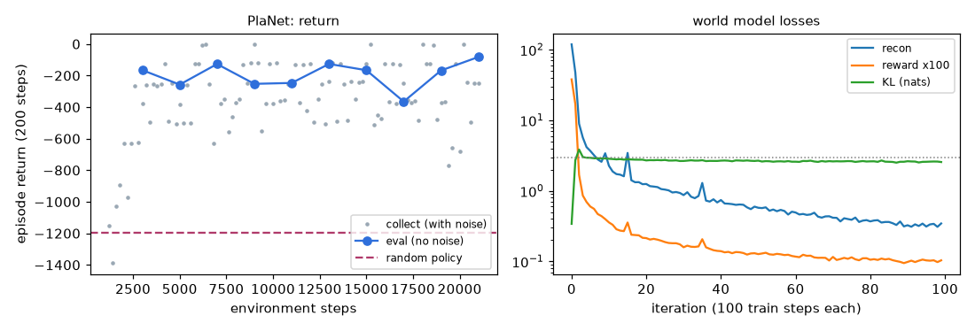
- Figure: Episode return and World Model loss curves (Figure 11-4)
- It learns from little data. After only 3,000 environment steps (15 episodes, about two and a half minutes of experience), the evaluation return reached −166. Random actions score −1194.
- The reconstruction loss fell from 119 to 0.35. The model learns the background within the first few iterations, then slowly refines the details of the bar.
- The KL starts at 0.3, quickly rises to around 3, and stays just below it (around 2.6). It is near 0 at first because the posterior barely uses the image yet, and it grows as reconstruction pulls the posterior toward the image. Below 3, free nats switch off the gradient, so it hovers near this "free allowance".
- Episodes with exploration noise are widely scattered, from near 0 to around −800. The noise \(\mathcal{N}(0, 0.3^2)\) amounts to about ±0.6 in torque, so it sometimes knocks the pendulum over while it is balancing at the top. Thanks to this, data on falling situations is collected as well.
Imagination vs. reality
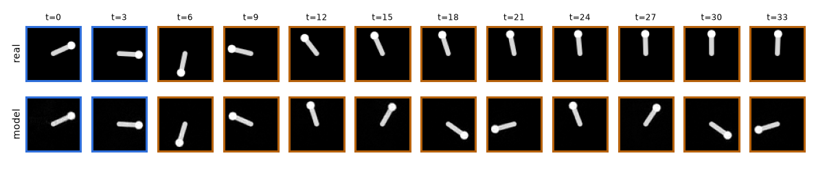
- Figure: Real images compared with images imagined by the RSSM (Figure 11-5)
- Frames t = 0 to 4 are redrawn by the decoder from states inferred by the posterior while seeing the images; from t = 5 on, the prior imagines them without seeing any images, given only the actions actually taken (one frame shown every 3 steps).
- After seeing five frames, the model imagines the pendulum falling down and swinging back up (t = 6 to 12) almost exactly as in reality. This is because it read the velocity, which no single image contains, from the five frames and stored it in \(h_t\).
- Around t = 15 the two diverge. The real pendulum stays upright at the top, while the imagined one overshoots the top and falls over. The causes are error accumulation (the prior only practiced one-step prediction) and the fact that the top is an unstable equilibrium where small differences change the outcome.
- Planning needs only 12 steps ahead, and within that range the imagination is accurate enough. MPC corrects the belief state with a new image at every moment and replans, so imagination errors about the distant future do not accumulate.
Swinging the pendulum up by planning
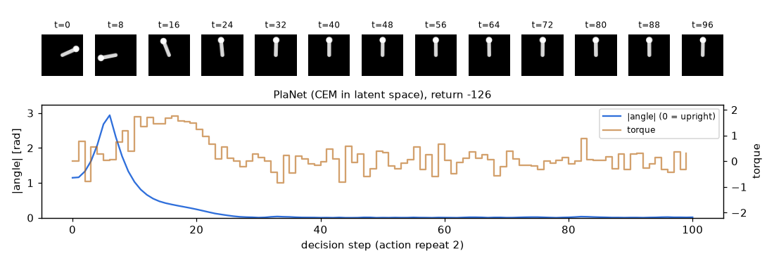
- Figure: An episode in which PlaNet swings the pendulum upright by planning (Figure 11-6, return −126)
- The pendulum starts tilted about 1.15 rad from the top. PlaNet does not push it straight up; it first lets the pendulum fall (\(\vert\theta\vert\) grows to nearly 3 rad over decisions 0 to 6). The torque is too weak to lift it directly, so it builds momentum at the bottom.
- It then pushes up with near-maximum torque (decisions 8 to 18) and balances at the top with small torques (\(\vert\theta\vert \approx 0\) after decision 25).
- Nobody taught it this "swinging" strategy; it was found solely by 12-step planning in imagination.
Performance and time
These values come from evaluation on 10 unseen start states (the final eval over 10 episodes line in main). The final test return on the last output line and Figures 11-5 and 11-6 come from the first episode of a freshly created evaluation environment with the same seed.
| Policy | Mean return (10 episodes) | Standard deviation | Min / max |
| Random actions | −1194.5 | - | - |
| PlaNet (21,000 environment steps) | −196.8 | 113.7 | −376.2 / −0.5 |
Returns vary widely across episodes because of the start position. Starting near the top gives nearly 0 (−0.5), while starting at the very bottom incurs angle penalties during the swing-up and gives −250 to −380. A mean of −150 to −200 means the task is essentially solved.
| Item | Value |
| Total training time (laptop GPU, shared with other training) | 4,535 s ≈ 76 min |
| Planning time (one decision, GPU) | About 100 ms on average; about 10 s per episode (100 decisions) |
| One World Model training step (CPU, 4 threads, \(B = 50\)) | About 17 s. The main settings (10,000 steps) are practically infeasible on CPU |
| Same, with | About 5 s. Over half a day for 10,000 steps |
| | About 1 min (only for checking that the code runs; no real learning) |
Without a GPU, use --quick to check that the code runs to completion, and do the actual training on a free cloud GPU (e.g. Google Colab). The three files to upload are wm_envs.py, ch11_rssm_planet.py, and ch12_dreamer.py.
Common problems
| Symptom | Common cause | What to try |
| Reconstructed images show only the black background, with no bar | The bar is only a small part of the image, so early on, fitting the background alone reduces the loss a lot | Train longer; the bar appears after a few thousand steps. If that does not help, lower the learning rate |
| The KL drops to near 0 and the imagination is a mess | Posterior collapse: the posterior ignores the image | Check that free nats are enabled ( |
| The imagination (open loop) blurs within a few steps | The prior only practiced one-step prediction; not enough data | Collect more data. Latent overshooting, a longer \(L\) |
| Planned actions turn out wrong in reality | The reward model is still inaccurate, or the planner "exploits" model errors | Check the reward loss. Keep the exploration noise. The problem shrinks as data accumulates |
| Too slow on CPU | Convolutions on 2500 images × backpropagation | |
Summary
- Images alone do not reveal velocity (partial observability), so a belief state that summarizes the past is needed. A latent state-space model learns it.
- The RSSM splits the state into a deterministic state \(h_t\) (GRU, memory) and a stochastic state \(z_t\) (Gaussian, uncertainty). Its five components are the GRU, the prior, the posterior, the observation decoder, and the reward decoder.
- The training objective is the sequential ELBO = \(\sum_t\) (reconstruction + reward − KL(posterior ‖ prior)). It is derived from the factorization of the joint distribution, Jensen's inequality, and splitting the expectation over time.
- The KL term is the only path that teaches the prior (the dynamics). Free nats switch off the gradient when the KL is below 3 nats, preventing posterior collapse.
- PlaNet plans in latent space with CEM (\(H=12\), \(I=10\), \(J=1000\), \(K=100\)) and executes only the first action (MPC). It is an expensive method that rolls the RSSM forward 120,000 steps per decision; Dreamer in chapter 12 removes this cost by learning a policy directly inside the same RSSM's imagination.
Review questions
- Question 1. What goes wrong if you remove \(h_t\) from the RSSM and keep only the stochastic state, or conversely remove \(z_t\)?
- Removing \(h_t\) (a pure stochastic SSM) forces all information through sampling at every step, which makes it hard to carry information accurately across many steps. Removing \(z_t\) (a deterministic RNN) means only one future can be represented, so branching futures are averaged into a blurry prediction, and with no latent variable the model cannot be trained with the ELBO and KL either.
- Question 2. In the derivation of the sequential ELBO, on which line does the inequality first appear, and what is required for equality?
- On the line that applies Jensen's inequality, \(\log \mathbb{E}[X] \ge \mathbb{E}[\log X]\). The gap is \(D_{\mathrm{KL}}(q(z_{1:T} \mid o_{1:T}) \parallel p(z_{1:T} \mid o_{1:T}, r_{1:T}))\), so equality holds when \(q\) equals the true posterior.
- Question 3. If the prior and the posterior are both \(\mathcal{N}(0.2,\ 0.5^2)\), what is the KL, and what are the loss and gradient with free nats of 3?
- The KL is \(\log(0.5/0.5) + (0.25 + 0)/(2 \cdot 0.25) - 0.5 = 0\). The free nats loss is \(\max(0, 3) = 3\), and the gradient is 0 in this region.
- Question 4. If the CEM candidates are reduced to \(J = 100\) and the elites to \(K = 10\), how many RSSM steps are rolled out per decision, and what is lost?
- \(10 \times 12 \times 100 = 12{,}000\) steps, a tenfold reduction. Fewer action sequences are examined per iteration, so the chance of finding a good action sequence drops, especially in the first few iterations, and plan quality may suffer (
--quickuses these values of \(J\) and \(K\) and also reduces the iterations to \(I = 3\)). - Question 5. If
reward_scaleis changed from 0.1 to 1, do the actions CEM chooses change? - If the reward model is accurate, they do not. CEM selects elites by the ranking of reward sums, and multiplying all rewards by the same positive constant leaves the ranking unchanged. During training, however, the reward loss becomes 100 times larger, which changes its balance with the other losses, so what the model learns may differ somewhat.
See also
- World Models:Tutorial
- World Models
- World Models:Tutorial:08 VAE
- World Models:Tutorial:07 MPC and CEM
- World Models:Tutorial:12 Dreamer
- VAE
- GRU
- Recurrent neural network
- Markov decision process
- Reinforcement learning