WorldModels:Tutorial:10-HaWorldModels
lastmod 2026-11-18created 2026-11-172 edits
World Models (Ha & Schmidhuber) is Chapter 10 of the World Model tutorial. On top of the eyes (V, a VAE) from Chapter 8 and the memory (M, an MDN-RNN) from Chapter 9, it adds a linear controller (C) with 289 parameters and reproduces David Ha and Jürgen Schmidhuber's 2018 World Models on the pendulum task. The controller is trained with an evolution strategy (CMA-ES) instead of gradients. The chapter compares a controller trained in the real environment with one trained only inside the dream generated by M, and covers the temperature τ, model exploitation, iterative training, and the limits of this approach.
- Original: 10. World Models (Ha & Schmidhuber)
- Example code:
code/ch10_world_models.py(about 15 minutes in total on a laptop GPU, about 1 hour on 4 CPU threads;--quickruns a smoke test. Run Chapters 8 and 9 first to producech08_vae.pt,ch09_mdnrnn.pt, andch09_latents.npz) - Previous: 09. RNN and MDN-RNN / Next: 11. RSSM and PlaNet
World Models in 2018
"World Models" (Ha & Schmidhuber, 2018) was published as an interactive web article that readers could run themselves, and it is the paper that popularized the term "world model". The same work appeared at NeurIPS 2018 under the title "Recurrent World Models Facilitate Policy Evolution". The paper showed two things.
| Task | Training method | Result | Threshold |
| CarRacing (top-down car racing, 64×64 image input) | A single linear controller on top of the features produced by V and M | Average of 906 ± 21 over 100 trials | 900 points (the first result to pass the score at which the task counts as "solved") |
| VizDoom: Take Cover (dodging incoming fireballs) | Random actions in the real game are used only to collect data; the controller is trained entirely inside the dream generated by M (dream temperature \(\tau = 1.15\)) | Survived 1092 ± 556 steps on average over 100 runs in the real game | 750 steps |
The second experiment matters more. It demonstrated that once you learn a model of the world, you can learn behavior inside that model purely through imagination. This idea leads to PlaNet in Chapter 11 and Dreamer in Chapter 12.
The V-M-C architecture
The image \(o_t\) from the environment passes through V to become \(z_t\) (32 dimensions). \(z_t\) and M's memory \(h_t\) (256 dimensions) go into C, which outputs the action \(a_t\) (a torque). \(a_t\) goes to the environment, and at the same time \(z_t, a_t\) go into M to update its memory. Each step comes down to three lines.
\(\begin{align} z_t &= \mu_\phi(o_t) && \text{V: image to latent vector (mean only)} \\ a_t &= C\big([z_t;\ h_t]\big) && \text{C: choose action from current scene + memory} \\ h_{t+1} &= \text{LSTM}\big([z_t;\ a_t],\ h_t\big) && \text{M: update memory} \end{align}\)
\(z_t\) captures what is visible right now, and \(h_t\) captures how things have moved so far and what is likely to come next. As shown in Chapter 9, \(h_t\) contains the pendulum's velocity, so C gets information that a single image cannot provide. Because M was trained to predict the next \(z\), its hidden state summarizes the information needed to predict the future, and the original paper also stresses that \(h_t\) encodes predictions about the future.
Training order
The three parts are trained separately, one after another.
- Collect episodes in the real environment with a random policy. (Chapter 8: 200 episodes)
- Train V on the collected images. (Chapter 8: ELBO)
- Train M on the \(z\) sequences produced by V. (Chapter 9: mixture NLL + reward MSE)
- Freeze V and M, and train C with an evolution strategy to maximize the return. (This chapter)
- If needed, collect new episodes with C and repeat steps 1–4.
Sizes in the original paper and the pendulum version
In the original paper (CarRacing), V maps a 64×64 color image to \(z \in \mathbb{R}^{32}\), and M is an LSTM with 256 hidden units and a 5-component mixture. This matches Chapters 8 and 9 of the tutorial. However, M in the original paper does not predict rewards: in CarRacing it predicts only the next \(z\), and in VizDoom it predicts the next \(z\) and whether the agent died (done). Because the pendulum's reward changes at every step, the tutorial added a reward head in Chapter 9.
C is a single linear function.
\(a_t = W_c\,[z_t;\ h_t] + b_c\)
| Item | Shape | Parameters |
| Input \([z_t;\ h_t]\) | \(32 + 256 = 288\) | |
| CarRacing (actions: steering, gas, brake) | \(W_c \in \mathbb{R}^{3 \times 288},\ b_c \in \mathbb{R}^{3}\) | \(288 \times 3 + 3 = 867\) |
| Pendulum (action: a single torque) | \(W_c \in \mathbb{R}^{1 \times 288},\ b_c \in \mathbb{R}\) | \(288 + 1 = 289\) |
To fit the torque range \([-2, 2]\), the controller in this chapter wraps the output in \(2\tanh\): \(a_t = 2\tanh(W_c[z_t;h_t] + b_c)\).
Compared with V (about 4.35 million) and M (about 420,000), C's 289 parameters are tiny. This is the design philosophy of World Models: the hard work of understanding the world is done by the large V and M through self-supervised learning (from data alone, without rewards), while the job of deciding what to do is left to the small C. This minimizes the number of parameters that must be learned from the sparse reward signal.
Why evolution strategies
The goal of training C is to maximize the expected episode return. Treat the parameters as a vector \(\theta \in \mathbb{R}^{289}\), and let \(F(\theta)\) be the return obtained by running an episode with that controller.
\(\max_\theta\; F(\theta),\qquad F(\theta) = \mathbb{E}\Big[\sum_{t=0}^{T-1} r_t \;\Big\vert\; \text{controller } \theta\Big]\)
Gradient descent needs \(\nabla_\theta F\), but \(F\) is a number that comes out of the real environment's physics, image rendering, and random initial states, so it is a box that cannot be differentiated. All you can do is feed in \(\theta\), run it, and get a single number back. This kind of problem is called black-box optimization.
Evolution strategies (ES) repeatedly generate a number of random offspring near the current parameters and move toward the offspring that score well. No gradient formula is needed, and since the offspring are evaluated independently, they can run in parallel. On the other hand, random search becomes inefficient once the parameters number in the millions. That is why World Models keeps C small.
C could also be trained with the policy gradient (REINFORCE) from Chapter 5. That method also works with non-differentiable environments, and the ES gradient formula derived below comes from the same log-derivative trick as the policy gradient. The difference is where the randomness is injected: the policy gradient adds noise to the actions, while ES adds noise to the parameters.
Deriving the evolution strategy gradient
Gaussian smoothing
Since \(F\) cannot be differentiated directly, the objective becomes the average of \(F\) over a Gaussian blur around \(\theta\). This is called Gaussian smoothing.
\(J(\theta) = \mathbb{E}_{\epsilon \sim \mathcal{N}(0, I)}\big[F(\theta + \sigma\epsilon)\big]\)
When \(\sigma\) is small, \(J(\theta) \approx F(\theta)\), and \(J\) is a smooth function even if \(F\) is bumpy or non-differentiable. The gradient of \(J\) can be computed from values of \(F\) alone.
\(\begin{align} J(\theta) &= \mathbb{E}_{x \sim \mathcal{N}(\theta,\ \sigma^2 I)}\big[F(x)\big] = \int F(x)\,p_\theta(x)\,dx \\ \nabla_\theta J(\theta) &= \int F(x)\,\nabla_\theta\, p_\theta(x)\,dx \\ &= \int p_\theta(x)\,F(x)\,\nabla_\theta\log p_\theta(x)\,dx = \mathbb{E}_{x \sim p_\theta}\big[F(x)\,\nabla_\theta\log p_\theta(x)\big] \\ &= \frac{1}{\sigma}\,\mathbb{E}_{\epsilon \sim \mathcal{N}(0,I)}\big[F(\theta + \sigma\epsilon)\,\epsilon\big] \;\approx\; \frac{1}{N\sigma}\sum_{i=1}^{N} F(\theta + \sigma\epsilon_i)\,\epsilon_i \end{align}\)
The justification for each line is as follows.
- Setting \(x = \theta + \sigma\epsilon\), \(x\) follows a Gaussian with mean \(\theta\) and covariance \(\sigma^2 I\) (the reparameterization from Chapter 8 viewed in reverse). Its density is \(p_\theta(x)\). Now \(\theta\) sits inside the distribution rather than inside \(F\).
- Move the derivative inside the integral. \(F(x)\) does not depend on \(\theta\), so only \(p_\theta(x)\) is differentiated. There is no longer any need to differentiate \(F\).
- Apply the log-derivative trick \(\nabla_\theta\, p_\theta(x) = p_\theta(x)\,\nabla_\theta \log p_\theta(x)\) and rewrite using the definition of expectation. This has the same form as the policy gradient in Chapter 5.
- The log density of a Gaussian with covariance \(\sigma^2 I\) is \(\log p_\theta(x) = -\frac{\lVert x - \theta\rVert^2}{2\sigma^2} + \text{const}\), so \(\nabla_\theta\log p_\theta(x) = \frac{x - \theta}{\sigma^2} = \frac{\sigma\epsilon}{\sigma^2} = \frac{\epsilon}{\sigma}\). Finally, the expectation is estimated by Monte Carlo.
The result means this: if moving in the noise direction \(\epsilon_i\) gave a high score, that direction gets a large weight; if it gave a low score, the update leans the opposite way. Only values of \(F\) are needed.
A numerical check
In one dimension, let \(F(x) = -(x - 3)^2\) (maximum at \(x = 3\)), \(\theta = 0\), and \(\sigma = 1\). Computing directly, \(\mathbb{E}[\epsilon] = 0\) and \(\mathbb{E}[\epsilon^2] = 1\) give \(J(\theta) = \mathbb{E}[-(\theta + \epsilon - 3)^2] = -(\theta-3)^2 - 1\), so \(J'(0) = -2(0 - 3) = 6\). Computing with the formula gives the following.
\(\begin{align} \frac{1}{\sigma}\mathbb{E}\big[F(0 + \epsilon)\,\epsilon\big] &= \mathbb{E}\big[-(\epsilon - 3)^2\,\epsilon\big] = -\mathbb{E}\big[\epsilon^3 - 6\epsilon^2 + 9\epsilon\big] \\ &= -\big(\mathbb{E}[\epsilon^3] - 6\,\mathbb{E}[\epsilon^2] + 9\,\mathbb{E}[\epsilon]\big) = -(0 - 6 + 0) = 6 \end{align}\)
The standard normal distribution is symmetric about 0, so its odd moments are 0. The result matches the value 6 obtained by direct differentiation.
Reducing variance
With few samples, this estimate is very noisy. In practice the following techniques are used together.
- Baseline subtraction: since \(\mathbb{E}[\epsilon] = 0\), for any constant \(b\) we have \(\mathbb{E}[(F - b)\,\epsilon] = \mathbb{E}[F\epsilon] - b\,\mathbb{E}[\epsilon] = \mathbb{E}[F\epsilon]\). The expectation stays the same, but choosing \(b\) as the mean score leaves only whether each sample did better or worse than average, which greatly reduces the variance (the same idea as the baseline in Chapter 5).
- Antithetic sampling: evaluate \(\epsilon\) and \(-\epsilon\) as a pair and compare them symmetrically.
- Fitness shaping: use ranks instead of raw scores, so a single outlier score does not throw off the estimate. CMA-ES uses only ranks.
CMA-ES
CMA-ES (covariance matrix adaptation evolution strategy) (Hansen & Ostermeier, 2001) is the most widely used evolution strategy. It sets the search distribution to \(\mathcal{N}(m,\ \sigma^2 C)\) and learns three things.
- Mean \(m\)
- Where to search.
- Covariance \(C\)
- Along which directions to stretch the search.
- Step size \(\sigma\)
- How widely to search.
Each generation, it samples and evaluates \(\lambda\) candidates and updates all three using only the top \(\mu\). It ignores the magnitudes of the scores and uses only their ranks. Because of conventions in the CMA-ES literature, some symbols overlap with earlier ones. In this section, \(C\) is the covariance matrix rather than the controller, \(\mu\) is the number of parents rather than a mean, \(\lambda\) is the number of candidates, and \(\sigma\) is the overall step size rather than a standard deviation.
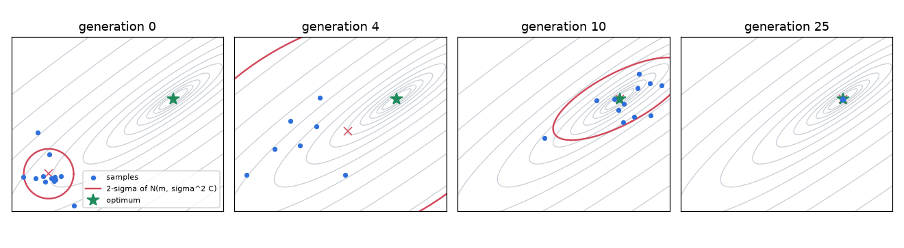
Running it on a tilted, elongated bowl-shaped 2D function with 12 candidates per generation: by generation 4, several generations have kept stepping in the same direction (up and to the right), so \(\sigma\) has grown and the 2-sigma ellipse has swollen; by generation 10, the ellipse has stretched diagonally along the bowl's orientation; and by generation 25, it has converged on the optimum and become very small.
Step 1: Sampling
\(x_k = m + \sigma\,y_k,\qquad y_k \sim \mathcal{N}(0, C),\qquad k = 1, \dots, \lambda\)
Keep the eigendecomposition \(C = B D^2 B^\top\) and build \(y_k = B D\,\epsilon_k\) (\(\epsilon_k \sim \mathcal{N}(0, I)\)). \(B\) is the orthogonal matrix whose columns are the eigenvectors, and \(D\) is the diagonal matrix of the square roots of the eigenvalues. This is correct because \(\operatorname{Cov}(BD\epsilon) = BD\,\operatorname{Cov}(\epsilon)\,(BD)^\top = BD\,I\,DB^\top = BD^2B^\top = C\).
Step 2: Moving the mean (weighted recombination)
Sort the candidates by score and write the step of the \(i\)-th best candidate as \(y_{i:\lambda}\). The mean is moved by weighting the top \(\mu = \lambda/2\) candidates.
\(m \leftarrow \sum_{i=1}^{\mu} w_i\,x_{i:\lambda} = m + \sigma\,y_w,\qquad y_w = \sum_{i=1}^{\mu} w_i\,y_{i:\lambda},\qquad w_i = \frac{\ln(\mu + \tfrac12) - \ln i}{\sum_{j=1}^{\mu}\big(\ln(\mu+\tfrac12) - \ln j\big)}\)
- Since \(x_{i:\lambda} = m + \sigma y_{i:\lambda}\) and \(\sum_i w_i = 1\), we get \(\sum_i w_i x_{i:\lambda} = m + \sigma y_w\).
- The weight is largest for first place and decreases toward place \(\mu\). With this chapter's settings (\(\lambda = 32\), \(\mu = 16\)), the weights for places 1–5 are 0.198, 0.149, 0.120, 0.100, and 0.084.
- The mean moves to the weighted average position of the good candidates. This is the same idea as CEM in Chapter 7, which moved to the (equally weighted) mean of the top candidates.
- When the weights are uneven, the number of candidates that effectively contribute to the mean is smaller than \(\mu\). This effective count is \(\mu_{\text{eff}} = 1/\sum_i w_i^2\). If all weights are \(1/\mu\), then \(\mu_{\text{eff}} = \mu\); if all the weight falls on one candidate, it is 1. With this chapter's settings, \(\mu_{\text{eff}} \approx 9.18\).
Step 3: Learning the covariance (rank-μ update)
Look at how the successful steps were spread out, and reshape the search distribution to match. That shape is found by maximum likelihood from Chapter 2. In one dimension, find the variance \(v\) that best explains the top steps \(y_1, \dots, y_\mu\) (with mean 0) using the weighted log-likelihood.
\(\begin{align} \max_{v}\; \sum_{i=1}^{\mu} w_i \log\mathcal{N}\big(y_i;\ 0,\ v\big) &= \sum_{i=1}^{\mu} w_i\Big(-\tfrac{1}{2}\log(2\pi v) - \frac{y_i^2}{2v}\Big) \\ \frac{\partial}{\partial v} &= \sum_{i=1}^{\mu} w_i\Big(-\frac{1}{2v} + \frac{y_i^2}{2v^2}\Big) = 0 \\ \sum_i w_i\,v &= \sum_i w_i\,y_i^2 \\ v &= \sum_{i=1}^{\mu} w_i\,y_i^2 \end{align}\)
Since \(\sum_i w_i = 1\), the variance is the weighted average of the squares. In multiple dimensions, the same calculation becomes a weighted average of outer products.
\(C_\mu = \sum_{i=1}^{\mu} w_i\,y_{i:\lambda}\,y_{i:\lambda}^\top\)
CMA-ES does not replace the covariance with this \(C_\mu\) all at once. Instead, it blends it gradually into the previous covariance as an exponential moving average with learning rate \(c_\mu\).
\(C \leftarrow (1 - c_1 - c_\mu)\,C + c_1\,p_c\,p_c^\top + c_\mu\sum_{i=1}^{\mu} w_i\,y_{i:\lambda}\,y_{i:\lambda}^\top\)
The third term is the rank-μ update, and the second term is the rank-1 update built from the evolution path \(p_c\). Setting \(c_1 = 0\), \(c_\mu = 1\) and making all weights equal gives almost the same form as CEM in Chapter 7. The differences are that CEM measures the variance around the new mean rather than the old one, that Chapter 7 measured it separately for each component, and that CEM has no separate step size \(\sigma\). CEM replaces the covariance wholesale every generation to fit the top samples, so it narrows quickly; CMA-ES changes it slowly, so it is stable.
Step 4: Evolution paths and step size
Accumulating the step \(y_w\) by which the mean moves each generation gives the evolution path.
\(p \leftarrow (1 - c)\,p + \sqrt{c\,(2 - c)\,\mu_{\text{eff}}}\;y_w\)
The factor \((1-c)\) gradually forgets the old path while the new step is added. The coefficient \(\sqrt{c(2-c)\mu_{\text{eff}}}\) is chosen so that the distribution of the path stays unchanged when selection is meaningless (when the scores are random). If the scores are random, the top \(\mu\) are also independent \(\mathcal{N}(0, C)\) samples, so the following holds.
\(\begin{align} \operatorname{Cov}(y_w) &= \sum_{i=1}^{\mu} w_i^2\,\operatorname{Cov}(y_i) = \Big(\sum_i w_i^2\Big)C = \frac{C}{\mu_{\text{eff}}} \\ \operatorname{Cov}(p_{\text{new}}) &= (1-c)^2\,\operatorname{Cov}(p) + c(2-c)\,\mu_{\text{eff}}\cdot\frac{C}{\mu_{\text{eff}}} \\ \operatorname{Cov}(p) = C \;&\Rightarrow\; \operatorname{Cov}(p_{\text{new}}) = \big((1-c)^2 + c(2-c)\big)C = (1 - 2c + c^2 + 2c - c^2)\,C = C \end{align}\)
The old path and the new step are independent, so their covariances add, and constant factors come out squared. If the old path was \(\mathcal{N}(0, C)\), the new path is also exactly \(\mathcal{N}(0, C)\), so you can fairly compare whether the path is longer or shorter than it would be by chance.
The step size \(\sigma\) is controlled on this principle (cumulative step-size adaptation, CSA). If you build a path \(p_\sigma\) with the shape of \(C\) removed (accumulating the steps multiplied by \(C^{-1/2}\)), then by chance \(p_\sigma \sim \mathcal{N}(0, I)\), and its expected length is \(\mathbb{E}\lVert\mathcal{N}(0,I)\rVert \approx \sqrt{n}\big(1 - \frac{1}{4n} + \frac{1}{21n^2}\big)\) (about 16.99 for this chapter's \(n = 289\)).
\(\sigma \leftarrow \sigma\cdot\exp\!\left(\frac{c_\sigma}{d_\sigma}\left(\frac{\lVert p_\sigma\rVert}{\mathbb{E}\lVert\mathcal{N}(0,I)\rVert} - 1\right)\right)\)
\(c_\sigma\) is the learning rate for accumulating the path, and \(d_\sigma\) is a damping constant that divides the update so that \(\sigma\) does not change too much in one generation. Its default is \(1 + 2\max\!\big(0,\ \sqrt{(\mu_{\text{eff}}-1)/(n+1)} - 1\big) + c_\sigma\) (about 1.04 in this chapter).
- If the path is longer than expected, several generations have kept walking in the same direction, which means the step is too small. The term in parentheses becomes positive and \(\sigma\) grows.
- If the path is shorter than expected, steps back and forth have canceled each other out, which means the step is large enough to overshoot the optimum. \(\sigma\) shrinks.
The covariance path \(p_c\) is accumulated in the same way but without multiplying by \(C^{-1/2}\), and the rank-1 update \(p_c p_c^\top\) imprints into the covariance the direction in which recent generations have consistently moved.
Default learning rates and the curse of dimensionality
| Value | Formula (Hansen's defaults) | 2D, λ = 12 | 289D, λ = 32 |
| \(\mu_{\text{eff}}\) | \(1/\sum w_i^2\) | 3.73 | 9.18 |
| \(c_\sigma\) | \(\frac{\mu_{\text{eff}}+2}{n+\mu_{\text{eff}}+5}\) | 0.534 | 0.0369 |
| \(c_c\) | \(\frac{4+\mu_{\text{eff}}/n}{n+4+2\mu_{\text{eff}}/n}\) | 0.603 | 0.0138 |
| \(c_1\) | \(\frac{2}{(n+1.3)^2+\mu_{\text{eff}}}\) | 0.137 | 0.0000237 |
| \(c_\mu\) | \(\min\!\big(1-c_1,\ \frac{2(\mu_{\text{eff}}-2+1/\mu_{\text{eff}})}{(n+2)^2+\mu_{\text{eff}}}\big)\) | 0.202 | 0.000172 |
The covariance learning rates \(c_1, c_\mu\) are inversely proportional to the square of the dimension \(n\). In 2D, about 34% (\(c_1 + c_\mu\)) of the covariance is renewed each generation (which is why the ellipse in Figure 10-2 tilts within a few generations), but in 289 dimensions less than 0.02% changes per generation. The covariance matrix has about \(n^2/2 \approx 42{,}000\) entries, so learning it reliably takes a correspondingly large number of generations. When run for only a few dozen generations, as in this chapter, CMA-ES effectively behaves as an evolution strategy that moves the mean by a rank-weighted average and adapts only the step size. That still works well enough.
numpy implementation
This is the cmaes section of ch10_world_models.py. It maximizes the objective: xs = es.ask() returns the candidates (λ, n), and es.tell(xs, fitness) passes back their fitness (higher is better). First, initialization.
class CMAES:
    def __init__(self, x0, sigma0: float, popsize: int | None = None, seed: int = 0):
        self.rng = np.random.default_rng(seed)
        n = len(x0)
        self.n = n
        self.mean = np.array(x0, dtype=np.float64)  # 분포의 평균 m
        self.sigma = float(sigma0)  # 전체 스텝 크기 σ
        self.lam = popsize or 4 + int(3 * np.log(n))  # 한 세대의 후보 수 λ
        self.mu = self.lam // 2  # 부모(상위) 수 μ
        w = np.log(self.mu + 0.5) - np.log(np.arange(1, self.mu + 1))  # 1등이 가장 큰 가중치
        self.weights = w / w.sum()
        self.mu_eff = 1.0 / np.sum(self.weights**2)  # 유효 부모 수
        # 학습률들 (기본값)
        self.c_sigma = (self.mu_eff + 2) / (n + self.mu_eff + 5)
        self.d_sigma = 1 + 2 * max(0.0, np.sqrt((self.mu_eff - 1) / (n + 1)) - 1) + self.c_sigma
        self.c_c = (4 + self.mu_eff / n) / (n + 4 + 2 * self.mu_eff / n)
        self.c_1 = 2 / ((n + 1.3) ** 2 + self.mu_eff)
        self.c_mu = min(1 - self.c_1, 2 * (self.mu_eff - 2 + 1 / self.mu_eff) / ((n + 2) ** 2 + self.mu_eff))
        self.chi_n = np.sqrt(n) * (1 - 1 / (4 * n) + 1 / (21 * n**2))  # E‖N(0, I)‖
        # 상태: 공분산 C = B diag(D²) Bᵀ, 진화 경로 p_σ, p_c
        self.C = np.eye(n)
        self.B = np.eye(n)
        self.D = np.ones(n)
        self.p_sigma = np.zeros(n)
        self.p_c = np.zeros(n)
        self.gen = 0
ask is Step 1, and tell is Steps 2–4.
    def ask(self):
        """x_k = m + σ · B D ε_k,  ε_k ~ N(0, I)   →  x_k ~ N(m, σ² C)."""
        eps = self.rng.standard_normal((self.lam, self.n))
        self.y = (eps * self.D) @ self.B.T  # y_k ~ N(0, C)
        return self.mean + self.sigma * self.y

    def tell(self, xs, fitness):
        order = np.argsort(-np.asarray(fitness))  # 큰 것부터
        y_best = self.y[order[: self.mu]]  # 상위 μ 개의 스텝 (μ, n)
        y_w = self.weights @ y_best  # 가중 평균 스텝
        # (1) 평균 갱신: 좋은 후보 쪽으로 옮긴다
        self.mean = self.mean + self.sigma * y_w
        # (2) 스텝 크기 σ: 진화 경로 p_σ 가 '우연' 보다 길면 키우고, 짧으면 줄인다
        C_inv_sqrt = self.B @ np.diag(1 / self.D) @ self.B.T
        self.p_sigma = (1 - self.c_sigma) * self.p_sigma + np.sqrt(
            self.c_sigma * (2 - self.c_sigma) * self.mu_eff) * (C_inv_sqrt @ y_w)
        norm_ps = np.linalg.norm(self.p_sigma)
        h_sigma = norm_ps / np.sqrt(1 - (1 - self.c_sigma) ** (2 * (self.gen + 1))) < (1.4 + 2 / (self.n + 1)) * self.chi_n
        # (3) 공분산 C: 진화 경로(rank-1) + 상위 스텝들의 가중 공분산(rank-μ)
        self.p_c = (1 - self.c_c) * self.p_c + h_sigma * np.sqrt(self.c_c * (2 - self.c_c) * self.mu_eff) * y_w
        rank_one = np.outer(self.p_c, self.p_c)
        rank_mu = (y_best.T * self.weights) @ y_best
        delta = (1 - h_sigma) * self.c_c * (2 - self.c_c)
        self.C = (1 - self.c_1 - self.c_mu) * self.C + self.c_1 * (rank_one + delta * self.C) + self.c_mu * rank_mu
        self.sigma *= np.exp((self.c_sigma / self.d_sigma) * (norm_ps / self.chi_n - 1))
        # C = B D² Bᵀ 고유값 분해 (대칭 · 양의 정부호 유지)
        self.C = np.triu(self.C) + np.triu(self.C, 1).T
        eigvals, self.B = np.linalg.eigh(self.C)
        self.D = np.sqrt(np.maximum(eigvals, 1e-20))
        self.gen += 1
| Math | Code |
| \(y_k = BD\epsilon_k,\ x_k = m + \sigma y_k\) | |
| Sort by score, take the top \(\mu\) | |
| \(y_w = \sum_i w_i y_{i:\lambda}\), \(m \leftarrow m + \sigma y_w\) | |
| \(p_\sigma \leftarrow (1-c_\sigma)p_\sigma + \sqrt{c_\sigma(2-c_\sigma)\mu_{\text{eff}}}\,C^{-1/2}y_w\) | |
| \(\sum_i w_i\,y_{i:\lambda}y_{i:\lambda}^\top\) | |
| \(\sigma \leftarrow \sigma\exp(\frac{c_\sigma}{d_\sigma}(\frac{\lVert p_\sigma\rVert}{\mathbb{E}\lVert N\rVert} - 1))\) | |
| \(C = BD^2B^\top\) | |
-
h_sigmais a safeguard: when \(p_\sigma\) is unusually long (while \(\sigma\) is growing quickly because the step size is too small), it briefly pauses the update of \(p_c\) to keep \(C\) from stretching excessively in one direction.deltais a term that makes up for the variance lost during that pause. - This implementation follows the basic algorithm in Hansen's "The CMA Evolution Strategy: A Tutorial". It omits only the negative weights for the lower-ranked candidates, which are the default in recent versions, and uses just the \(\mu\) positive weights. In practice, you can use the
cmapackage.
Controller and rollouts
Controller
A single CMA-ES candidate is 289 numbers. These are split into \(W_c\) (288) and \(b_c\) (1) and used as a controller. A batched matrix multiplication (bmm) computes \(P\) candidates at once.
class Controllers:
    """후보 P 개의 선형 컨트롤러를 한꺼번에 계산한다.

    params: (P, n) numpy, n = (z_dim + hidden) · 1 + 1   (가중치 W 와 편향 b 를 이어 붙인 것)
    act(feat): feat (P, K, F) → 행동 (P, K, 1) = 2 · tanh(feat · W + b)
    """

    def __init__(self, params, feat_dim: int, device):
        p = torch.as_tensor(params, dtype=torch.float32, device=device)
        self.W = p[:, :feat_dim].unsqueeze(-1)  # (P, F, 1)
        self.b = p[:, feat_dim:].unsqueeze(1)  # (P, 1, 1)

    def act(self, feat):
        return 2.0 * torch.tanh(torch.bmm(feat, self.W) + self.b)  # (P, K, 1)
Rollouts in the real environment
\(P\) candidates × \(K\) initial states, for \(P\cdot K\) pendulums in total, run simultaneously. At each step, all images go through the VAE in one batch, the controllers choose actions, each pendulum advances one step, and the MDN-RNN updates the memory. When the real environment is used, M is used only to build the memory \(h_t\), not to predict the future.
@torch.no_grad()
def rollout_real(params, seeds, vae, mdn, device, record=False):
    """진짜 환경에서 후보 P 개 × 시작 상태 K 개를 동시에 돌린다. 반환: 리턴 (P, K).

    매 스텝: 그림 o_t → V: z_t = μ_φ(o_t) → C: a_t = C([z_t ; h_t]) → 환경 · M 갱신 h_{t+1}
    """
    P, K = len(params), len(seeds)
    ctrl = Controllers(params, mdn.z_dim + mdn.hidden, device)
    envs = [PixelPendulum(seed=int(s)) for _ in range(P) for s in seeds]
    obs = np.stack([env.reset() for env in envs])  # (P·K, 64, 64)
    state = mdn.initial_state(P * K, device)
    returns = np.zeros(P * K)
    frames, thetas = [], []
    for t in range(200):
        z, _ = vae.encode(to_float(obs, device))  # (P·K, D)  평균 μ 를 z 로 쓴다
        h = state[0][0]  # (P·K, H)  행동 전의 기억 h_t
        feat = torch.cat([z, h], dim=-1).view(P, K, -1)
        a = ctrl.act(feat).view(P * K, 1)  # (P·K, 1)
        a_np = a.cpu().numpy()
        if record:
            frames.append(obs[0].copy())
            thetas.append([env.th for env in envs])
        results = [env.step(a_np[i]) for i, env in enumerate(envs)]
        obs = np.stack([r[0] for r in results])
        returns += np.array([r[1] for r in results])
        _, _, _, _, state = mdn(z.unsqueeze(1), a.unsqueeze(1), state)  # M 이 기억을 갱신
    if record:
        return returns.reshape(P, K), np.stack(frames), np.array(thetas)
    return returns.reshape(P, K)
- The mean \(\mu\) from
vae.encode(...)is used as \(z\). A noise-free value works better when choosing actions. -
h = state[0][0]takes \(h\) out of the LSTM state \((h, c)\) with the layer axis removed; it is the memory \(h_t\) before the action. - All candidates in a generation are evaluated from the same initial states (the same
seeds). This variance-reduction technique, called common random numbers, ensures that candidate A beats B because of its parameters rather than a lucky initial state. Each generation draws new initial states to prevent overfitting to particular ones.
Rollouts in the dream
The real environment is removed. M samples the next \(z\), and the reward also comes from M's reward head. Since there is no image rendering and no VAE pass, this is very fast, and thousands of rollouts can run at once on the GPU.
@torch.no_grad()
def rollout_dream(params, z0, mdn, device, tau: float, steps: int = 200):
    """꿈속 롤아웃: 진짜 환경 없이 M 이 다음 z 와 보상을 지어낸다. 반환: 꿈속 리턴 (P, K).

    z0: (K, D) 시작 그림들의 z (진짜 에피소드의 첫 장면에서 가져온다)
    """
    P, K = len(params), len(z0)
    ctrl = Controllers(params, mdn.z_dim + mdn.hidden, device)
    z = torch.as_tensor(z0, device=device).repeat(P, 1)  # (P·K, D)
    state = mdn.initial_state(P * K, device)
    returns = torch.zeros(P * K, device=device)
    for t in range(steps):
        h = state[0][0]
        a = ctrl.act(torch.cat([z, h], dim=-1).view(P, K, -1)).view(P * K, 1)
        log_pi, mu, log_sigma, r_hat, state = mdn(z.unsqueeze(1), a.unsqueeze(1), state)
        returns += r_hat[:, 0]  # 보상도 M 이 지어낸 것
        z = mdn_sample(log_pi[:, 0], mu[:, 0], log_sigma[:, 0], tau)  # 다음 z 를 뽑아 다시 입력
    return returns.view(P, K).cpu().numpy()
The first scene of each dream is chosen from the \(z\) values that the VAE produced from the first images of real episodes (z_starts, mu[:, 0] in ch09_latents.npz). Everything after that is imagined. Only two lines differ from the real rollout: the reward comes from r_hat instead of the environment, and the next \(z\) comes from mdn_sample(..., tau) instead of the VAE.
Training loop
def train_controller(mode, vae, mdn, z_starts, device, generations=60, popsize=32, rollouts=4, sigma0=0.1,
                     tau=1.0, eval_every=5, eval_seeds=None, seed=0, log=print):
    """CMA-ES 로 컨트롤러를 학습한다. mode = 'real' (진짜 환경) 또는 'dream' (꿈속).

    매 세대: 후보 popsize 개 × 시작 상태 rollouts 개를 돌려 '평균 리턴' 을 적합도로 쓴다.
    eval_every 세대마다 '현재 평균 m' 을 진짜 환경의 고정 시작 상태들(eval_seeds)로 평가한다.
    """
    n = mdn.z_dim + mdn.hidden + 1
    es = CMAES(np.zeros(n), sigma0, popsize, seed=seed)
    rng = np.random.default_rng(seed + 100)
    history = []  # (세대, 적합도 평균, 적합도 최고, 진짜 평가 리턴 또는 nan)
    for g in range(generations + 1):
        xs = es.ask()
        if mode == "real":
            seeds = rng.integers(0, 10**6, rollouts)  # 세대마다 새 시작 상태, 후보끼리는 같게
            fit = rollout_real(xs, seeds, vae, mdn, device).mean(axis=1)
        else:
            z0 = z_starts[rng.integers(0, len(z_starts), rollouts)]
            fit = rollout_dream(xs, z0, mdn, device, tau).mean(axis=1)
        es.tell(xs, fit)
        real_eval = np.nan
        if g % eval_every == 0 or g == generations:
            real_eval = rollout_real(es.mean[None], eval_seeds, vae, mdn, device).mean()
            log(f"[{mode}{'' if mode == 'real' else f' τ={tau:g}'}] 세대 {g:3d} | 적합도 평균 {fit.mean():8.1f} "
                f"최고 {fit.max():8.1f} | σ {es.sigma:.3f} | 진짜 환경 평가(평균 m) {real_eval:8.1f}")
        history.append((g, fit.mean(), fit.max(), real_eval))
    return es.mean, np.array(history)
| Item | Real-environment training (A) | Dream training (B) | Original paper |
| Number of candidates \(\lambda\) ( | 32 | 32 | 64 |
| Rollouts per candidate \(K\) | 4 ( | 16 ( | 16 |
| Generations | 60 ( | 150 ( | |
| Temperature τ | N/A | 0.1, 1.0, 1.5 ( | |
| Real-environment evaluation interval | Every 5 generations | Every 10 generations | |
| Initial \(m\), \(\sigma\) | \(m = 0\), | ||
Each generation runs candidates × initial states and uses the mean return as the fitness. Even when training happens in the dream, every few generations the current mean \(m\) is evaluated on 20 fixed initial states in the real environment (eval_seeds, 1000–1019) and logged. These evaluation values are not used for training; they serve only to check whether dream training actually works.
Results: real-environment training vs. dream training
The code trains a controller four times on the same V and M: (A) 60 generations in the real environment (4 episodes per candidate), and (B) 150 generations each in the dream at temperatures τ = 0.1, 1.0, and 1.5 (16 dreams per candidate). Since the code counts from generation 0, the actual numbers of updates are 61 and 151, and the number of episodes in (A) is 61 × 32 × 4 = 7,808.
장치: cuda
컨트롤러 매개변수 수: (32 + 256) × 1 + 1 = 289
기준선 | 무작위 행동 -1226.9 | 토크 0 -1251.6
[real] 세대   0 | 적합도 평균  -1328.2 최고  -1147.2 | σ 0.097 | 진짜 환경 평가(평균 m)  -1210.7
[real] 세대  10 | 적합도 평균  -1086.7 최고   -820.0 | σ 0.085 | 진짜 환경 평가(평균 m)   -776.0
…
[real] 세대  60 | 적합도 평균   -580.4 최고   -321.1 | σ 0.086 | 진짜 환경 평가(평균 m)   -301.7
(A) 진짜 환경 학습 356초 | 학습에 쓴 진짜 에피소드 7808개 (1,561,600 스텝)
[dream τ=0.1] 세대   0 | 적합도 평균  -1258.8 최고  -1061.9 | σ 0.097 | 진짜 환경 평가(평균 m)  -1184.1
…
[dream τ=0.1] 세대 150 | 적합도 평균   -383.7 최고   -244.4 | σ 0.104 | 진짜 환경 평가(평균 m)   -315.6
(B) 꿈속 학습 τ=0.1 174초
…
[dream τ=1] 세대 150 | 적합도 평균   -334.8 최고   -204.7 | σ 0.104 | 진짜 환경 평가(평균 m)   -278.6
(B) 꿈속 학습 τ=1 177초
…
[dream τ=1.5] 세대 150 | 적합도 평균   -419.9 최고   -230.6 | σ 0.097 | 진짜 환경 평가(평균 m)   -306.1
(B) 꿈속 학습 τ=1.5 176초

최종 평가 (진짜 환경: 고정 시작 상태 20개 평균 ± 표준편차, 꿈속: 학습 때와 같은 τ, 시작 상태 64개)
  real       | 꿈속 리턴   -488.1 | 진짜 리턴   -301.7 ± 181.1
  dream 0.1  | 꿈속 리턴   -268.0 | 진짜 리턴   -315.6 ± 197.2
  dream 1    | 꿈속 리턴   -238.9 | 진짜 리턴   -278.6 ± 144.4
  dream 1.5  | 꿈속 리턴   -289.6 | 진짜 리턴   -306.1 ± 203.7
그림 저장: figures
Time and the amount of real experience
- In the environment where the tutorial was written (a laptop GPU shared with other training jobs), the whole run took about 15 minutes: 356 seconds for real-environment training and about 175 seconds per temperature for dream training.
- Dream training finished in half the time despite having 2.5 times as many generations and 4 times as many evaluations per candidate. On the real-environment side, even with a GPU, most of the time goes to the Python loop that advances 128 pendulums (32 candidates × 4 initial states) one step at a time and renders their images.
- With only a CPU (4 threads), one real-environment generation takes about 26 seconds and one dream generation takes a few seconds, for about 1 hour in total.
- The more important difference is the amount of real experience. (A) used 7,808 real episodes (about 1.56 million steps) for training, while (B) used no real environment for training at all apart from the 200 episodes (40,000 steps) collected at random in Chapter 8.
Learning curves
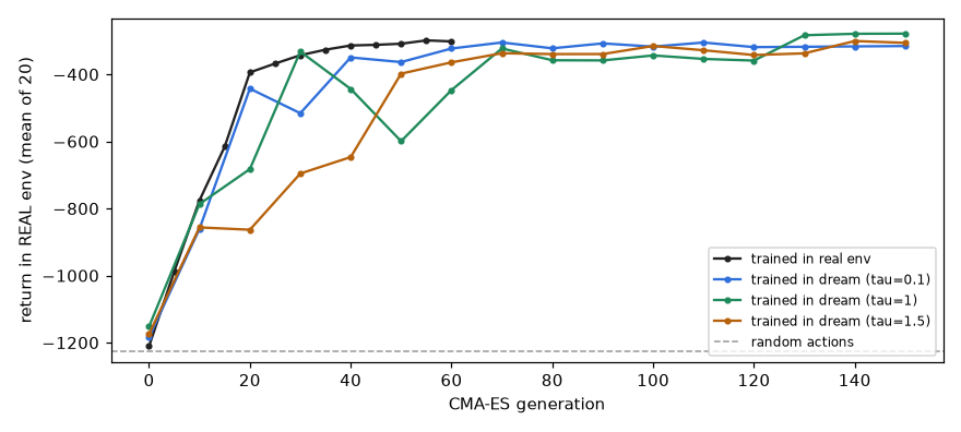
This plots the real-environment evaluation return (mean over 20 fixed initial states) against generation.
- Real-environment training starts at the random-action level (about −1210) and climbs to −302 within 60 generations. Because it receives scores directly from the real world, it makes the fastest progress per generation. This shows that a linear controller with just 289 numbers learned to look at images and balance the pendulum upright.
- Dream training at all three temperatures also starts at the random level and reaches −279 to −316 after 150 generations, on par with the controller trained in the real environment. These controllers never experienced the real pendulum during training.
- The τ = 1 curve drops sharply midway (around generation 50) and then recovers. The dream scores themselves are noisy, so the CMA-ES mean drifted in the wrong direction for a while. The more random the dream, the more the same candidate's score varies from evaluation to evaluation, so it is important to average over plenty of dreams per candidate (16 here).
- Figure: Figure 10-3. Real-environment evaluation return per generation for real-environment training and dream training at three temperatures
Dream return vs. real return
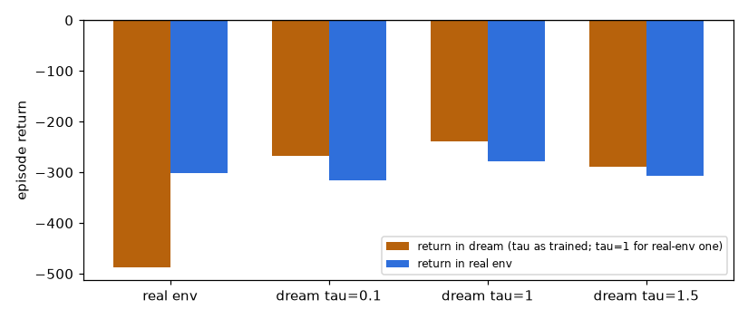
Each controller was evaluated in the dream (at its training τ, or τ = 1 for the controller trained in the real environment, with 64 initial states) and in the real environment.
| Controller | Dream return | Real return (mean ± std) | Dream − real |
| Real-environment training | −488.1 | −301.7 ± 181.1 | Dream is much worse |
| Dream τ = 0.1 | −268.0 | −315.6 ± 197.2 | 48 |
| Dream τ = 1 | −238.9 | −278.6 ± 144.4 | 40 |
| Dream τ = 1.5 | −289.6 | −306.1 ± 203.7 | 16 |
- All three controllers trained in the dream have a slightly better dream return than real return. This signals that the dream is a little more optimistic than reality and that the controllers are exploiting small loopholes in the dream. In this run, the gap shrank as τ increased (48 → 40 → 16).
- Conversely, the controller trained in the real environment scores −488 in the dream (τ = 1), much worse than in reality (−302). The dream and reality are not the same world, and a controller tuned to one does not carry over unchanged to the other.
- One possible reason is the collapsed dimensions seen in Chapter 9. In real rollouts, images are mapped to the mean \(\mu\), so the 25 collapsed dimensions always stay near 0, but in the τ = 1 dream those dimensions are sampled as \(\mathcal{N}(0,1)\) noise. A controller trained only in the real environment had no reason to clean up its weights on those dimensions, so it gets thrown off by the noise in the dream, whereas the controllers trained in the dream presumably learned to ignore that noise.
- Figure: Figure 10-4. Bar chart of the dream and real returns of the four controllers
A single run should not be trusted on its own. Below are the results of rerunning only the dream-training part with different random seeds.
| Setting (dream training) | Dream return | Real return |
| Run above: τ = 0.1 / 1 / 1.5, 150 generations, 16 dreams per candidate | −268 / −239 / −290 | −316 / −279 / −306 |
| Rerun with different seeds only: τ = 0.1 / 1 / 1 / 1.5, 150 generations, 16 dreams | −257 / −286 / −270 / −305 | −263 / −338 / −312 / −329 |
| First attempt: τ = 0.1 / 1 / 1.5, 60 generations, 4 dreams | −507 / −338 / −892 | −568 / −381 / −854 |
- With 150 generations and 16 dreams, every run produced a usable controller with a real return of −260 to −340, and the dream was always optimistic by 6 to 52.
- The differences between temperatures are small enough to flip from run to run, so it is not possible to say which τ is best for this pendulum.
- The last row is the setting first tried while preparing the tutorial (60 generations, 4 dreams per candidate). With too few generations and too few evaluations, dream training is far less stable, which is why the default settings were increased.
A controller trained in the dream balances the real pendulum
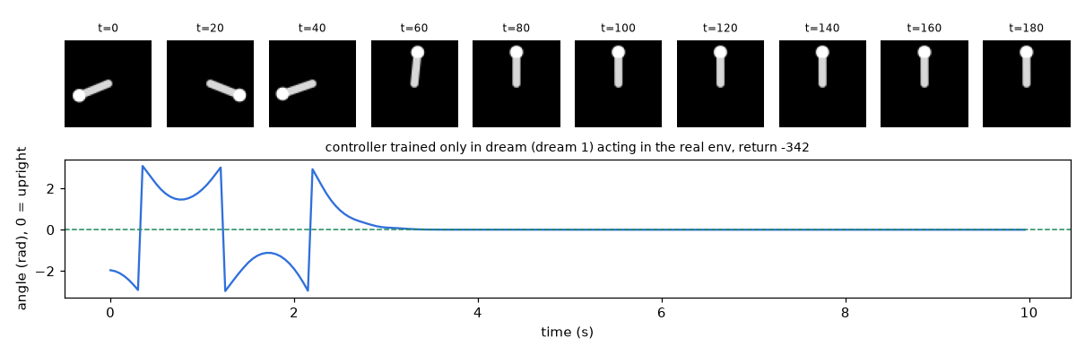
The controller with the best real return among those trained only in the dream (τ = 1) was placed in the real environment from one evaluation initial state that was not used in training. Over roughly the first 2 seconds, the controller swings the pendulum widely left and right twice to build up energy, raises it to the top on the third swing, and holds it upright from about 3 seconds until the end (10 seconds). Using only images, it discovered in the dream the crux of the pendulum problem: the torque is too weak to lift the pendulum in one go. In the angle plot, the points where the value jumps between \(+\pi\) and \(-\pi\) are the moments when the pendulum passes the very bottom (the hanging position). The return from this initial state is −342. The return is far from 0 because of the large angle penalties during the first 3 seconds of swinging up; after the pendulum is upright, the penalty is nearly 0.
Temperature and cheating in the dream
Training in the dream carries a fundamental risk: the controller will find anything that raises the return. If M makes wrong predictions in some situation (for example, if it wrongly believes that applying torque a certain way makes the pendulum stop at the top), the controller learns to exploit that error instead of learning the real physics. This is called model exploitation, or in the original paper's words, cheating inside the dream. A controller with a high dream score but a low real score is the symptom.
Ha & Schmidhuber demonstrated this directly in the VizDoom experiment.
| Dream temperature | Dream score | Real game score |
| Low (e.g., 0.1) | 2086 ± 140 (maximum 2100) | 193 ± 58 |
| 1.15 | 1092 ± 556 |
In a nearly deterministic dream, M could not switch to the mixture component in which a fireball is created and flies toward the agent (mode collapse), so the monsters in the dream never shot fireballs at all. In a dream with no danger, any controller gets a nearly perfect score but learns nothing. Raising the temperature to 1.15 made the dream more uncertain and harder than reality, so cheats that exploited M's loopholes no longer worked every time. The controller learned behavior that holds up whatever future comes, and that behavior also worked in the real game.
For the pendulum, the temperature did not make that much difference. The dream was slightly optimistic at every temperature, but dream training worked in reality even at low temperature. The likely reasons are as follows.
- The world is simple. The pendulum's physics is deterministic and smooth, so M learns it almost exactly (Chapter 9: error under 8° after 25 steps). There are few loopholes to begin with.
- The data covers the state space evenly. Episodes start from random angles, so the data contains a fair number of images near the top.
- The controller is small. A linear controller is not expressive enough to precisely exploit subtle loopholes in M.
VizDoom was the opposite: the scenes are complex, fireballs arrive in random patterns, and there are many situations that random actions never reach. The effect of temperature grows the more easily the model can be wrong about the world.
The quality of dream training depends not only on how closely the dream resembles reality but also on whether the controller can exploit loopholes in the dream. Raising the temperature to make the dream uncertain is the simplest way to signal "do not trust the model where it does not know", and it serves the same purpose as the ensemble (PETS) handling uncertainty in Chapter 7. The way to reduce the places where the model is wrong in the first place is iterative training.
Iterative training
V and M in this chapter were trained only on data collected with random actions. But a good controller goes where random actions rarely go. For the pendulum, that means staying nearly still at the top for several seconds (over a hundred steps). If such states are rare in the training data, M is likely to be wrong there, and that is where model exploitation happens. It is even more serious in tasks like CarRacing, where random actions never even reach the end of the track.
Ha & Schmidhuber proposed the following iterative training procedure. The original mentions only M and C; the steps below are spelled out for the tutorial's V, M, and C (exploration noise and retraining V are additions).
- Initialize M and C randomly.
- Collect episodes in the real environment with the current C (plus some exploration noise) and add them to the data.
- Retrain V and M on the accumulated data.
- Retrain C inside the dream of the new M.
- Go back to step 2 until the task is solved.
This steadily increases the data from wherever the controller goes, so M learns those regions accurately and the loopholes that cheating relied on get closed. This is the same structure as the model-based reinforcement learning in Chapters 6 and 7, which alternated between collecting data and training the model. PlaNet and Dreamer in Chapters 11 and 12 make this loop the basic structure of their training.
To try this with this chapter's code, pass the controller as the policy to Chapter 8's collect_pixel_episodes(n, policy=...) to collect episodes (the policy must reset its LSTM memory to 0 at the start of each episode), merge that data with the Chapter 8 data, rerun train_vae and train_mdnrnn, and then call train_controller("dream", ...) again.
Limitations of World Models
- V does not know the task. The VAE only learns what is needed to reconstruct the image, not what is relevant to the reward. It ignores objects that matter but occupy few pixels, such as a small ball, and spends capacity on things that do not matter but occupy many pixels, such as the background.
- V, M, and C are trained separately. M's errors are not passed back to V, and C's needs are not passed back to M. Training all three together would let them adapt to one another.
- C has to be small. CMA-ES slows down sharply once there are more than a few thousand parameters (the covariance learning rate shrinks as \(1/n^2\)). Simpler evolution strategies that do not learn a covariance are also used for larger neural networks, but they need many samples. Complex behavior requires a large policy.
- Gradients are not used inside the dream. Even though M is a differentiable neural network, C learns only from scores. If the policy could be improved directly by differentiating through the whole dream, much more could be learned from the same dream.
The RSSM in Chapter 11 merges V and M into a single probabilistic model trained jointly, and PlaNet plans at every step inside that model. Dreamer in Chapter 12 differentiates through the entire dream of that model to train a large neural-network policy.
Summary
- World Models = V (VAE) + M (MDN-RNN) + C (a small controller). The large V and M learn through self-supervised learning without rewards, and the small C learns from the return alone with an evolution strategy.
- The evolution strategy gradient is \(\nabla_\theta\mathbb{E}[F(\theta+\sigma\epsilon)] = \frac{1}{\sigma}\mathbb{E}[F(\theta+\sigma\epsilon)\epsilon]\). It is computed from values of \(F\) alone and comes from the log-derivative trick.
- CMA-ES samples from \(\mathcal{N}(m, \sigma^2C)\) and updates \(m\) with the weighted average of the top candidates, \(C\) with the weighted covariance of the successful steps (maximum likelihood) and the evolution path, and \(\sigma\) with the path length.
- In a dream rollout, M generates the next \(z\) and the reward without the real environment. It is fast and parallelizable, but the controller can exploit the model's errors (model exploitation).
- Raising the temperature τ to make the dream uncertain makes exploitation harder. Regions with too little data are filled in by iterative training.
- In the pendulum experiment, controllers trained only in the dream (real return −279 to −316) performed on par with the controller trained on 7,808 episodes in the real environment (−302).
Exercises
- 1. Counting parameters: if \(z\) has 64 dimensions, the LSTM hidden size is 512, and the action is 2-dimensional, how many parameters does the linear controller have?
- \((64 + 512) \times 2 + 2 = 1154\).
- 2. ES gradient: with \(F(x) = -x^2\), \(\theta = 1\), and \(\sigma = 0.5\), compute \(\frac{1}{\sigma}\mathbb{E}[F(\theta + \sigma\epsilon)\epsilon]\) and compare it with the value obtained by differentiating \(J(\theta)\) directly.
- Since \(-(1 + 0.5\epsilon)^2\epsilon = -(\epsilon + \epsilon^2 + 0.25\epsilon^3)\), the expectation is \(-(0 + 1 + 0) = -1\), and \(\frac{1}{0.5}\times(-1) = -2\). Computing directly, \(J(\theta) = -(\theta^2 + \sigma^2)\) and \(J'(1) = -2\), so they match.
- 3. Effective number of parents: if the weights are \((0.5,\ 0.3,\ 0.2)\), what is \(\mu_{\text{eff}}\)?
- \(1/(0.25 + 0.09 + 0.04) = 1/0.38 \approx 2.63\). There are three parents, but in effect they count as about 2.6.
- 4. Step size: if the mean keeps moving forward and backward over several generations, what happens to the length of \(p_\sigma\) and to \(\sigma\)?
- Steps in opposite directions cancel each other out, so \(\lVert p_\sigma\rVert\) becomes shorter than the expected length. The term in parentheses becomes negative and \(\sigma\) shrinks. This signals that the step was large enough to overshoot the optimum.
- 5. Model exploitation: you obtained a controller with a very high dream return but a low real return. What are two likely causes, and how would you address them?
- (1) M's predictions were wrong in states absent from the training data (for example, holding steady at the top for a long time), and the controller learned to steer into those wrong regions. Collect new data with that controller and retrain M (iterative training). (2) The dream was too deterministic (τ too low), so small model errors were reproduced identically every time and got exploited. Raise τ to make the dream uncertain.
Things worth changing in experiments:
- Reduce to
--dream-rollouts 4 --dream-generations 60to see how unstable dream training becomes. - Change to
--taus 0.1,1.0,2.0or--popsize 64and compare how Figures 10-3 and 10-4 change. - To trigger model exploitation deliberately, rerun Chapter 8 with
--episodes 20and retrain Chapter 9 on that data to give M more loopholes, then run this chapter. Watch how the gap between the dream return and the real return changes with τ. - Replace the controller with a small MLP with 16 hidden units (which increases the number of parameters) and measure how much slower CMA-ES becomes.
See also
- World Models:Tutorial
- World Models
- Recurrent World Models Facilitate Policy Evolution
- VAE
- Mixture Density Network
- LSTM
- Reinforcement learning
- Maximum likelihood estimation