WorldModels:Tutorial:09-MDN-RNN
lastmod 2026-11-18created 2026-11-172 edits
Building Memory: RNN and MDN-RNN is Chapter 9 of the World Model tutorial. The VAE from Chapter 8 summarizes a single image as 32 numbers \(z\), but a single image does not say which way the pendulum is swinging or how fast. This chapter covers recurrent neural networks (RNNs) and LSTMs, which remember past frames, and mixture density networks (MDNs), which predict a future that is not uniquely determined as a probability distribution. Combining the two gives the MDN-RNN, a model that dreams the future in latent space. It corresponds to M (Memory) in Ha & Schmidhuber's World Models, and Chapter 10 builds on the model and latent sequences trained here.
- Original: 09. Building Memory: RNN and MDN-RNN
- Hands-on code:
code/ch09_mdn_rnn.py(about 2 min 20 s in total on a laptop GPU; with 4 CPU threads, training alone takes about 20 minutes.--quickruns a smoke test. Run Chapter 8 first to producech08_vae.ptandch08_episodes.npz.) - Previous: 08. VAE / Next: 10. Ha and Schmidhuber's World Models
One image is not enough
Two identical images of a rod tilted 45° to the right can come from very different situations: in one the rod is falling quickly clockwise, in the other it is almost at rest. The next frames are completely different, yet an agent that sees only one image cannot tell them apart. Chapter 5 called this situation partial observability and such a problem a POMDP: the observation \(o_t\) does not contain the full state \(s_t = (\theta, \dot\theta)\).
The fix is to look at past frames as well. The pendulum environment's physics updates the angle as \(\theta_t = \theta_{t-1} + \dot\theta_t\,\Delta t\) (Chapter 6), so dividing the angle difference between two frames by \(\Delta t = 0.05\) s gives the velocity exactly.
\(\dot\theta_t = \frac{\theta_t - \theta_{t-1}}{\Delta t}\)
In the general world two frames may not be enough (acceleration, occluded objects, events long ago), so we need a way to carry around "a summary of everything seen so far". That summary is the hidden state \(h_t\), and the neural network that updates it at every step is a recurrent neural network (RNN).
Recurrent neural networks (RNNs)
Equations
The most basic RNN (the Elman RNN) fits on one line.
\(h_t = \tanh\big(W_h\,h_{t-1} + W_x\,x_t + b\big),\qquad y_t = W_y\,h_t + c\)
- \(x_t\): the input at time \(t\). In the MDN-RNN it is \([z_t; a_t]\).
- \(h_{t-1}\): the memory up to the previous step. The initial \(h_0\) is the zero vector.
- \(W_h, W_x, b\): the same weights at every time step (parameter sharing). Because the same network is applied repeatedly, it works on sequences of any length.
- \(\tanh\): squashes the result into -1 to 1 so the memory cannot grow without bound.
- \(y_t\): the output (prediction) at that time step.
A numerical example
For a one-dimensional RNN with \(W_h = 0.5\), \(W_x = 1\), \(b = 0\) and input \(x = (1, 0, 0)\):
\(\begin{align} h_1 &= \tanh(0.5 \cdot 0 + 1 \cdot 1) = \tanh(1) \approx 0.762 \\ h_2 &= \tanh(0.5 \cdot 0.762 + 1 \cdot 0) = \tanh(0.381) \approx 0.363 \\ h_3 &= \tanh(0.5 \cdot 0.363) = \tanh(0.182) \approx 0.180 \end{align}\)
Even with zero input, about half of the previous memory survives, but it shrinks by roughly half at every step. This RNN remembers that it "saw a 1" for only a few steps. This fast forgetting has the same root as the vanishing gradient described below.
Unrolling through time
Unrolling an RNN along the time axis gives a deep network made of identical cells chained side by side. Starting from \(h_0 = 0\), each cell takes an input \(x_t\), emits an output \(y_t\), and passes its memory \(h_t\) to the cell on its right. All cells share the same weights, so a sequence of length \(T\) becomes a network of depth \(T\).
BPTT and vanishing/exploding gradients
Backpropagation back through time
An unrolled RNN is a deep network, so the backpropagation from Chapter 4 applies unchanged. Because the gradient flows backward in time, it is called BPTT (backpropagation through time) (Backpropagation through time). The loss is the sum of per-step losses \(L = \sum_t L_t\), and since the same \(W_h\) is used at every step, the gradient of \(W_h\) is the sum of contributions from all time steps.
The key question is how sensitive the loss at time \(T\) is to a much earlier memory \(h_k\), that is, \(\partial L_T / \partial h_k\). If this is small, the model cannot learn relationships between the distant past and the present. By the chain rule, we multiply the rates of change at every step (Jacobian matrices in the vector case).
\(\frac{\partial L_T}{\partial h_k} = \frac{\partial L_T}{\partial h_T}\,\frac{\partial h_T}{\partial h_{T-1}}\,\frac{\partial h_{T-1}}{\partial h_{T-2}}\cdots\frac{\partial h_{k+1}}{\partial h_k} = \frac{\partial L_T}{\partial h_T}\prod_{t=k+1}^{T}\frac{\partial h_t}{\partial h_{t-1}}\)
Within one step, write \(h_t = \tanh(a_t)\) with \(a_t = W_h h_{t-1} + W_x x_t + b\) (in this derivation \(a_t\) is the pre-activation value fed into tanh, not the action).
- Since \(\frac{d}{da}\tanh(a) = 1 - \tanh^2(a)\) and tanh is applied element-wise, \(\frac{\partial h_t}{\partial a_t} = \operatorname{diag}(1 - h_t^2)\).
- \(a_t\) is linear in \(h_{t-1}\), so \(\frac{\partial a_t}{\partial h_{t-1}} = W_h\).
\(\frac{\partial L_T}{\partial h_k} = \frac{\partial L_T}{\partial h_T}\prod_{t=k+1}^{T}\operatorname{diag}\big(1 - h_t^2\big)\,W_h\)
A matrix of the same form, \(\operatorname{diag}(1-h_t^2)W_h\), is multiplied \(T - k\) times. Since these are matrices, order matters: the \(t = T\) factor is leftmost and the \(t = k+1\) factor is rightmost. The longer the product, the more likely the result is to go to zero or blow up.
The derivative of tanh follows from the quotient rule: write \(\tanh a = N/D\) with \(N = e^{a} - e^{-a}\) and \(D = e^{a} + e^{-a}\), so that \(N' = D\) and \(D' = N\).
\(\Big(\frac{N}{D}\Big)' = \frac{N'D - ND'}{D^2} = \frac{D\cdot D - N\cdot N}{D^2} = 1 - \frac{N^2}{D^2} = 1 - \tanh^2 a\)
The closer \(\vert\tanh a\vert\) is to 1 (saturation), the closer the derivative is to 0.
Why gradients vanish or explode
In one dimension, if the factor \(w(1 - h_t^2)\) multiplied at each step has magnitude roughly \(\rho\), then after 20 steps the gradient is multiplied by \(\rho^{20}\).
| \(\rho\) | \(\rho^{20}\) | Effect |
| 0.5 | \(0.5^{20} \approx 9.5 \times 10^{-7}\) | Vanishing gradient (Gradient Vanishing). Events from 20 steps earlier leave almost no trace in the gradient. |
| 1.5 | \(1.5^{20} \approx 3325\) | Exploding gradient (Gradient Exploding). The gradient swells by a factor of thousands and a single update throws training off course. |
Since \(\tanh' = 1 - h^2 \le 1\), a saturated memory (\(\vert h\vert \to 1\)) makes the factor even smaller, so vanishing becomes more likely. In the vector case, the eigenvalues of the matrix \(W_h\) play the same role. An eigenvector \(v\) satisfies \(Wv = \lambda v\), so
\(W^2 v = W(\lambda v) = \lambda^2 v, \qquad W^n v = \lambda^n v\)
If the largest eigenvalue has magnitude less than 1, every direction shrinks to zero; if it is greater than 1, that direction explodes.
Gradient clipping
Explosion is prevented with gradient clipping. If the norm of the gradient vector \(g\) exceeds a threshold \(c\), its direction is kept and only its length is scaled down to \(c\).
\(g \leftarrow g\cdot\min\Big(1, \frac{c}{\lVert g\rVert}\Big)\)
The code in this chapter uses \(c = 1\) with a single line, clip_grad_norm_(model.parameters(), 1.0). Clipping does not fix vanishing gradients; that requires changing the network architecture, which is what the LSTM does.
LSTM: memory with gates
Equations and gates
The LSTM (long short-term memory) (Hochreiter & Schmidhuber, 1997) splits memory in two: the cell state \(c_t\), which stores information long-term, and the hidden state \(h_t\), which is exposed to the outside. Three gates decide what to erase from the cell state, what to write to it, and what to output. The original 1997 version had no forget gate; Gers et al. (2000) added it, and the form below is today's standard. \([h_{t-1}; x_t]\) is the concatenation of the two vectors, \(\sigma\) is the sigmoid \(\sigma(u) = \frac{1}{1+e^{-u}}\) (values in 0 to 1), and \(\odot\) is element-wise multiplication. In this section \(o_t\) is the output gate, not the observation, and \(\sigma\) means the sigmoid only in this section (from the MDN section on it is the standard deviation again).
\(\begin{align} f_t &= \sigma\big(W_f[h_{t-1}; x_t] + b_f\big) && \text{forget gate} \\ i_t &= \sigma\big(W_i[h_{t-1}; x_t] + b_i\big) && \text{input gate} \\ g_t &= \tanh\big(W_g[h_{t-1}; x_t] + b_g\big) && \text{candidate (new content to write)} \\ o_t &= \sigma\big(W_o[h_{t-1}; x_t] + b_o\big) && \text{output gate} \\ c_t &= f_t \odot c_{t-1} + i_t \odot g_t && \text{cell state update} \\ h_t &= o_t \odot \tanh(c_t) && \text{hidden state} \end{align}\)
- Forget gate \(f_t\): decides how much of each cell-state entry to keep (1 keeps everything, 0 erases everything).
- Input gate \(i_t\) and candidate \(g_t\): decide how much of the new information \(g_t\) to write.
- Output gate \(o_t\): decides which parts of the cell state to expose now (to the next layer and the output).
Gate values lie between 0 and 1, so the gates act like valves. Because they are differentiable, what to remember is itself learned from data. Structurally, the input \([h_{t-1}; x_t]\) feeds all three gates and the candidate, while the cell state \(c_{t-1} \to c_t\) flows along a straight path with only one multiplication (\(\times f_t\)) and one addition (\(+\, i_t \odot g_t\)). \(h_t\) is obtained by applying tanh to \(c_t\) and multiplying by \(o_t\).
Why the cell state preserves gradients
In the update \(c_t = f_t \odot c_{t-1} + i_t \odot g_t\), \(c_{t-1}\) appears directly only in the first term, and the derivative of an element-wise product is the factor it was multiplied by.
\(\frac{\partial c_t}{\partial c_{t-1}} \approx \operatorname{diag}(f_t), \qquad \frac{\partial c_T}{\partial c_k} \approx \prod_{t=k+1}^{T}\operatorname{diag}(f_t)\)
\(f_t, i_t, g_t\) are also indirectly connected to \(c_{t-1}\) through \(h_{t-1}\), but that path shrinks just like in an RNN, so here we look only at the direct path. Along the direct path, only the forget-gate values are multiplied in; neither a weight matrix nor \(\tanh'\) appears.
- If \(f_t \approx 1\), the gradient reaches the distant past almost unchanged. The update then becomes \(c_t \approx c_{t-1} + i_t\odot g_t\), adding new content to the old memory, and addition has derivative 1, so it does not shrink the gradient.
- An RNN overwrites its memory by multiplying by a matrix and squashing with tanh at every step, whereas an LSTM keeps a separate path that erases and adds only as much as needed. This additive path leads on to ResNet's residual connections and the Transformer's residual stream.
- In practice the forget-gate bias \(b_f\) is sometimes initialized to a positive value such as 1 so that the network starts out remembering well.
The parameter count is four groups (three gates plus the candidate \(g_t\)) × (weights + biases). With hidden size \(H = 256\) and input size \(X = 32 + 1 = 33\), that is \(4 \times (256 \times 33 + 256 \times 256 + 256 + 256) = 297{,}984\) (PyTorch keeps two sets of biases, one on the input side and one on the hidden side).
GRU
The GRU (gated recurrent unit) (Cho et al., 2014) merges the cell state and hidden state into one and reduces the gates to two.
\(\begin{align} u_t &= \sigma\big(W_u[h_{t-1}; x_t] + b_u\big) && \text{update gate} \\ r_t &= \sigma\big(W_r[h_{t-1}; x_t] + b_r\big) && \text{reset gate} \\ \tilde{h}_t &= \tanh\big(W_h[r_t \odot h_{t-1}; x_t] + b_h\big) && \text{candidate} \\ h_t &= u_t \odot h_{t-1} + (1 - u_t)\odot \tilde{h}_t && \text{mixing} \end{align}\)
The new memory is a weighted average of the old memory and the candidate; when \(u_t \approx 1\) the old memory passes through unchanged (the same effect as \(f_t \approx 1\) in the LSTM). It has three quarters of the LSTM's parameters and often performs about as well, which is why the RSSM in Chapter 11 (PlaNet, Dreamer) uses a GRU.
The equations above follow the published (EMNLP) version of Cho et al. (2014), and PyTorch's nn.GRU uses \(u\) in the same direction. There are two common variants.
- Some papers, such as Chung et al. (2014), flip the role of \(u\) and write \(h_t = (1-u_t)\odot h_{t-1} + u_t\odot\tilde h_t\).
- When computing the candidate, PyTorch does not multiply \(h_{t-1}\) by \(r_t\) first; it computes \(W h_{t-1}\) and then multiplies. This is the form that appeared in the first arXiv version (v1) of the Cho et al. paper.
A single answer versus a distribution
MSE fits the conditional mean
Before predicting the next latent vector \(z_{t+1}\) from the RNN's output, let us see what MSE regression, as in Chapter 6, actually fits. When the target \(y\) varies across several values for the same input \(x\), we minimize the expected squared error with a single prediction \(c\).
\(\frac{d}{dc}\mathbb{E}\big[(y - c)^2\big] = \mathbb{E}\big[-2(y - c)\big] = -2\big(\mathbb{E}[y] - c\big) = 0 \quad\Rightarrow\quad c^\ast = \mathbb{E}[y \mid x]\)
The second derivative is \(2 \gt 0\), so this is a minimum. A network trained with MSE outputs the average of the possible futures.
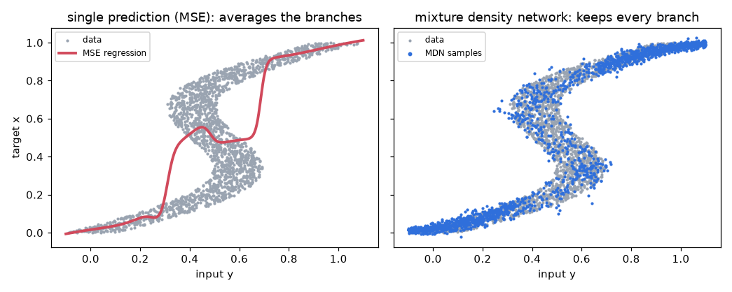
If the future is uniquely determined, the average is the answer. If the future branches, things change. A pendulum nearly at rest at the top can fall either left or right; if the target is one of two images with equal probability, the MSE answer is their average, a blurry image with two overlapping rods. That future never actually happens. In one dimension, if the target is \(\pm 1\) with equal probability, the MSE prediction is 0, a value that never occurs. If a World Model imagines such averaged futures, behavior learned on top of them goes wrong too, so the model must predict a distribution rather than a single value.
A toy problem
We use the classic example from Bishop (1994). Draw \(x\) from 0 to 1 and generate \(y = x + 0.3\sin(2\pi x) + \text{noise}\) (the code uses 2000 samples with noise uniform in ±0.1), then invert the task and predict \(x\) from \(y\). For \(y\) around 0.4 to 0.6, three different values of \(x\) produce such a \(y\).
- A network trained with MSE passes through the average of the branches, a region with almost no data. Samples drawn from a mixture density network follow all three branches.
- The run prints
[장난감] MSE 회귀 손실 0.0380 | MDN 음의 로그 가능도 -1.142: an MSE regression loss of 0.0380 and an MDN negative log-likelihood of -1.142 on the toy problem. An MSE loss of 0.038 means an average error of \(\sqrt{0.038} \approx 0.19\), which is large compared with the spread of the data. - A negative NLL for the MDN is not strange. The density of a continuous distribution can exceed 1 (at the peak of a narrow Gaussian), so the log density can be positive and the NLL negative.
- Figure: MSE regression line versus MDN samples (Figure 9-3)
Mixture density networks (MDNs)
A mixture of Gaussians
A mixture density network (MDN) (Bishop, 1994) outputs a mixture of \(K\) Gaussians instead of a single number (Mixture Density Network, Gaussian mixture model).
\(p(y \mid x) = \sum_{k=1}^{K} \pi_k(x)\;\mathcal{N}\big(y;\ \mu_k(x),\ \sigma_k^2(x)\big),\qquad \pi_k \ge 0,\ \ \sum_{k=1}^K \pi_k = 1\)
It is a sum of \(K\) bell curves weighted by \(\pi_k\), so it can have several peaks. For each input \(x\), the network outputs three numbers per component.
| Parameter | Network output | Transform |
| Mixture weight \(\pi_k\) | Logit \(\ell_k\) | Softmax \(\pi_k = \frac{e^{\ell_k}}{\sum_j e^{\ell_j}}\). Always positive and sums to exactly 1. |
| Mean \(\mu_k\) | \(\mu_k\) | Used as is. |
| Standard deviation \(\sigma_k\) | Log standard deviation \(\log\sigma_k\) | \(\sigma_k = e^{\log\sigma_k}\). Always positive. |
Here \(\pi_k\) is neither the circle constant nor a policy; it is the weight of the \(k\)-th component. Only the \(\pi\) inside \(\log 2\pi\) in the equations below is the circle constant.
When \(y\) is \(D\)-dimensional, Ha & Schmidhuber use a separate mixture of \(K\) components for each dimension.
\(p(y) = \prod_{d=1}^{D}\sum_k \pi_{d,k}\,\mathcal{N}(y_d;\mu_{d,k},\sigma_{d,k}^2)\)
So the number of outputs is \(3 \times K \times D\). With 32-dimensional \(z\) and \(K = 5\), that is \(3 \times 5 \times 32 = 480\).
Log-likelihood of a mixture
Training is maximum likelihood, i.e., minimizing the negative log-likelihood (NLL). The log of a sum cannot be split into a sum of logs, so we use \(u = \exp(\log u)\) to rewrite it in log-sum-exp form.
\(\begin{align} \log p(y \mid x) &= \log \sum_{k=1}^{K}\pi_k\,\mathcal{N}(y;\mu_k,\sigma_k^2) \\ &= \log \sum_{k=1}^{K}\exp\Big(\log\pi_k + \log\mathcal{N}(y;\mu_k,\sigma_k^2)\Big) \\ &= \operatorname{logsumexp}_{k}\big(a_k\big),\qquad a_k = \log\pi_k - \log\sigma_k - \tfrac{1}{2}\log 2\pi - \tfrac{1}{2}\Big(\frac{y - \mu_k}{\sigma_k}\Big)^2 \end{align}\)
Here \(\operatorname{logsumexp}(a) := \log\sum_k e^{a_k}\), and the last three terms of \(a_k\) are the Gaussian log density written out (\(\log\frac{1}{\sigma\sqrt{2\pi}} = -\log\sigma - \tfrac{1}{2}\log 2\pi\)).
Stabilizing log-sum-exp
Converting \(a_k\) directly to \(e^{a_k}\) is dangerous. If a prediction is even slightly off, \(a_k\) can be something like -1000, and in float32 \(e^{-1000}\) is exactly 0. If every component is 0, we get \(\log 0 = -\infty\) and training collapses. Conversely, a large \(a_k\) makes \(e^{a_k}\) overflow to infinity. The fix is to subtract the largest value \(m = \max_k a_k\) first.
\(\sum_{k} e^{a_k} = e^{m}\sum_k e^{a_k - m} \quad\Rightarrow\quad \log\sum_k e^{a_k} = m + \log\sum_k e^{a_k - m}\)
Since \(a_k - m \le 0\), we have \(e^{a_k - m} \le 1\), so nothing overflows; and since the largest term is \(e^0 = 1\), the sum is at least 1, so \(\log 0\) never occurs.
- Numerical example: computing \(a = (-1000,\ -1001)\) directly gives \(\log(0 + 0) = -\infty\). With stabilization, \(m = -1000\) and the result is \(-1000 + \log(e^0 + e^{-1}) = -1000 + \log(1.368) \approx -999.687\).
- PyTorch's
torch.logsumexpandF.log_softmaxuse this method. The log-softmax \(\log\pi_k = \ell_k - \operatorname{logsumexp}(\ell)\) relies on the same trick.
y.unsqueeze(-1) adds a component axis to the target so it can be compared with all \(K\) components at once (broadcasting), and logsumexp is taken over the last (component) axis.
def mdn_log_prob(y, log_pi, mu, log_sigma):
    """혼합 가우시안의 로그 가능도 log p(y) 를 log-sum-exp 로 안정하게 계산한다.

    y         : (..., D)      정답
    log_pi    : (..., D, K)   혼합 가중치의 로그 (log_softmax 결과)
    mu        : (..., D, K)   성분별 평균
    log_sigma : (..., D, K)   성분별 로그 표준편차
    반환       : (..., D)      차원마다의 log p(y_d)
    """
    y = y.unsqueeze(-1)  # (..., D, 1) → K 개 성분과 나란히 비교
    # 성분 k 의 로그 정규 밀도: -log σ - ½ log 2π - ½ ((y-μ)/σ)²
    log_normal = -log_sigma - 0.5 * LOG_2PI - 0.5 * ((y - mu) / log_sigma.exp()) ** 2
    # log Σ_k π_k N_k = logsumexp_k (log π_k + log N_k)
    return torch.logsumexp(log_pi + log_normal, dim=-1)
The toy-problem MDN has an output layer that emits three numbers per component (logit, mean, log standard deviation).
class ToyMDN(nn.Module):
    """입력 x (1차원) → 출력 y 의 혼합 가우시안 (K 개 성분)."""

    def __init__(self, n_mix: int = 5, hidden: int = 64):
        super().__init__()
        self.body = nn.Sequential(nn.Linear(1, hidden), nn.Tanh(), nn.Linear(hidden, hidden), nn.Tanh())
        self.head = nn.Linear(hidden, 3 * n_mix)  # 성분마다 (가중치 로짓, 평균, 로그 표준편차)

    def forward(self, x):
        logit_pi, mu, log_sigma = self.head(self.body(x)).chunk(3, dim=-1)  # 각각 (B, K)
        log_pi = F.log_softmax(logit_pi, dim=-1)  # 합이 1 이 되도록
        return log_pi.unsqueeze(1), mu.unsqueeze(1), log_sigma.clamp(-7, 3).unsqueeze(1)  # (B, 1, K)
Sampling with temperature
Sampling from a mixture takes two steps.
- Pick a component: choose component \(k\) with probabilities \(\pi_1, \dots, \pi_K\).
- Sample from that component: \(y = \mu_k + \sigma_k\,\epsilon\), \(\epsilon \sim \mathcal{N}(0, 1)\).
The resulting \(y\) is distributed as \(\sum_k P(k)\,p(y \mid k) = \sum_k\pi_k\mathcal{N}(y;\mu_k,\sigma_k^2)\), which is exactly the mixture (marginalization). Ha & Schmidhuber add a temperature \(\tau\) to control how random the dream is.
\(\pi_k^{(\tau)} = \frac{\exp(\log\pi_k/\tau)}{\sum_j\exp(\log\pi_j/\tau)} = \frac{\pi_k^{1/\tau}}{\sum_j \pi_j^{1/\tau}},\qquad y = \mu_k + \sigma_k\sqrt{\tau}\,\epsilon\)
| Temperature | Effect |
| \(\tau = 1\) | Exactly the distribution the model learned. |
| \(\tau \lt 1\) | Large components grow larger (sharper) and noise shrinks. As \(\tau \to 0\), the dream becomes noise-free, outputting only the mean of the largest component. |
| \(\tau \gt 1\) | Components are picked more evenly and noise grows. The dream is more uncertain and rougher. |
As a numerical example, take \(\pi = (0.7,\ 0.3)\). At \(\tau = 0.5\), raising to the power \(1/\tau = 2\) gives \((0.49,\ 0.09)\), and dividing by their sum 0.58 gives \((0.845,\ 0.155)\). At \(\tau = 2\), the square roots \((0.837,\ 0.548)\) divided by their sum 1.384 give \((0.604,\ 0.396)\). The higher the temperature, the closer the two components become. This \(\tau\) plays an important role in Chapter 10.
def mdn_sample(log_pi, mu, log_sigma, tau: float = 1.0):
    """온도 τ 로 혼합 가우시안에서 표본을 뽑는다 (Ha & Schmidhuber 의 방식).

    1) 성분 고르기: 확률 ∝ exp(log π_k / τ)   (τ 가 크면 고르게, 작으면 가장 큰 성분만)
    2) 그 성분에서 뽑기: μ_k + σ_k · √τ · ε
    τ = 0 이면 가장 큰 성분의 평균을 그대로 돌려준다 (잡음 없는 꿈).
    """
    if tau <= 1e-6:
        k = log_pi.argmax(dim=-1, keepdim=True)
        return mu.gather(-1, k).squeeze(-1)
    k = torch.distributions.Categorical(logits=log_pi / tau).sample().unsqueeze(-1)  # (..., D, 1)
    mu_k = mu.gather(-1, k).squeeze(-1)
    sigma_k = log_sigma.gather(-1, k).squeeze(-1).exp()
    return mu_k + sigma_k * math.sqrt(tau) * torch.randn_like(mu_k)
MDN-RNN: the M in World Models
Architecture
At each step the LSTM reads \([z_t; a_t]\) and updates its memory; from its output, the MDN head produces a mixture distribution over the next latent vector \(z_{t+1}\) and the reward head produces the reward \(r_t\) (Recurrent World Models Facilitate Policy Evolution).
\(\begin{align} (h_{t+1}, c_{t+1}) &= \text{LSTM}\big([z_t; a_t],\ (h_t, c_t)\big) \\ p_\theta(z_{t+1} \mid z_{\le t}, a_{\le t}) &= \prod_{d=1}^{32}\sum_{k=1}^{5}\pi_{d,k}\,\mathcal{N}\big(z_{t+1,d};\ \mu_{d,k},\ \sigma_{d,k}^2\big),\quad (\pi, \mu, \sigma) = \text{MDN}(h_{t+1}) \\ \hat{r}_t &= w_r^\top h_{t+1} + b_r \end{align}\)
The indexing convention differs from the previous sections. In the RNN and LSTM sections, \(h_t\) denoted the memory after reading input \(x_t\); from here on, following the original paper, the memory after reading \(z_t, a_t\) is written \(h_{t+1}\). So \(h_t\) is the memory before seeing \(z_t\), and this is why the controller in Chapter 10 takes \([z_t; h_t]\) together.
| Component | Size | Parameters |
| Input \(z_t\) (32) + \(a_t\) (1) | 33 | - |
| LSTM | Hidden 256 | 297,984 |
| MDN head (\(\pi, \mu, \sigma\)) | 256 → 480 = 3 × 5 × 32 | 123,360 |
| Reward head (\(\hat{r}_t\)) | 256 → 1 | 257 |
| Total | 421,601 |
The total parameter count is about a tenth of the Chapter 8 VAE (about 4.35 million). The memory \((h, c)\) carries hidden information such as velocity into the next step.
class MDNRNN(nn.Module):
    """M 모델: LSTM 이 (z_t, a_t) 를 읽고 z_{t+1} 의 혼합 가우시안과 보상 r_t 를 내놓는다.

    z 의 각 차원 d 마다 따로 K 개 성분의 혼합을 쓴다 (Ha & Schmidhuber 와 같다).
    """

    def __init__(self, z_dim: int = 32, act_dim: int = 1, hidden: int = 256, n_mix: int = 5):
        super().__init__()
        self.z_dim, self.act_dim, self.hidden, self.n_mix = z_dim, act_dim, hidden, n_mix
        self.lstm = nn.LSTM(z_dim + act_dim, hidden, batch_first=True)
        self.mdn_head = nn.Linear(hidden, 3 * z_dim * n_mix)  # 차원 · 성분마다 (로짓, μ, log σ)
        self.reward_head = nn.Linear(hidden, 1)

    def heads(self, out):
        """LSTM 출력 (B, T, H) → 혼합 매개변수 각각 (B, T, D, K), 보상 (B, T)."""
        B, T, _ = out.shape
        params = self.mdn_head(out).view(B, T, 3, self.z_dim, self.n_mix)
        logit_pi, mu, log_sigma = params.unbind(dim=2)
        log_pi = F.log_softmax(logit_pi, dim=-1)  # 성분 K 개에 대해 합 1
        log_sigma = log_sigma.clamp(-7.0, 2.0)  # 너무 작거나 큰 σ 막기 (수치 안정)
        reward = self.reward_head(out).squeeze(-1)
        return log_pi, mu, log_sigma, reward

    def forward(self, z, a, state=None):
        """z: (B, T, D), a: (B, T, A) → 혼합 매개변수, 보상, 새 LSTM 상태 (h, c)."""
        out, state = self.lstm(torch.cat([z, a], dim=-1), state)  # out: (B, T, H)
        return (*self.heads(out), state)

    def initial_state(self, batch: int, device):
        zeros = torch.zeros(1, batch, self.hidden, device=device)
        return (zeros, zeros.clone())
-
batch_first=Truemeans tensors are laid out as (batch, time, feature). -
view(B, T, 3, D, K)splits the output into (logit, μ, log σ) × 32 dimensions × 5 components, andunbind(dim=2)pulls out the three tensors. -
clamp(-7, 2)bounds \(\sigma\) between \(e^{-7} \approx 0.0009\) and \(e^{2} \approx 7.4\), preventing a component from narrowing into a needle and sending the NLL out of control. -
initial_stateis \((h_0, c_0) = (0, 0)\) at the start of an episode. The shape (number of layers 1, batch, hidden) is PyTorch's LSTM convention.
Training: teacher forcing and the loss
Every image in the 200 episodes is first converted to \(\mu, \log\sigma^2\) with the Chapter 8 VAE (encode_frames), and the MDN-RNN is trained on those sequences. The z sequences have shape (200, 201, 32), i.e., (episode, time, dimension).
\(\mathcal{L}(\theta) = \frac{1}{BL}\sum_{b=1}^{B}\sum_{t=1}^{L}\Big[-\sum_{d=1}^{32}\log p_\theta\big(z^{(b)}_{t+1,d}\big) + \lambda_r\big(\hat{r}^{(b)}_t - r^{(b)}_t\big)^2\Big]\)
The first term is the NLL of the next latent vector (summed over dimensions, averaged over time and batch), the second is the reward MSE, and \(\lambda_r = 1\).
- Teacher forcing
- During training, the LSTM's input is always the real \(z_t\). Even if the model mispredicted earlier, the next step receives the ground truth. This lets all time steps be computed at once (in parallel) and stabilizes training. When dreaming, however, the model receives its own predictions as input and so encounters slightly wrong inputs it never saw in training. This mismatch is called exposure bias, and it is one reason dreams drift further the longer they run (the same phenomenon as error accumulation in Chapter 6).
- A freshly sampled z every time
- Instead of fixing each image to its mean \(\mu\), a new \(z = \mu + \sigma\odot\epsilon\) is drawn for every batch (the same approach as Ha & Schmidhuber). Since the VAE encodes each image as a cloud, this is data augmentation that teaches the model to predict over the whole cloud.
- Truncated BPTT
- For each batch, an episode
epand a start timet0are chosen at random and a window of length 65 (= \(L + 1\)) is cut out. The input isz[:, :-1](indices 0 to 63) and the target isz[:, 1:](indices 1 to 64), offset by one so the model predicts "the next one". Because only a 64-step window is used rather than the full episode (200 steps), gradients flow back at most 64 steps. Even when a window starts in the middle of an episode, the memory starts at \((h, c) = (0, 0)\), so the first few steps of the window are predicted without knowing the velocity.
Hyperparameters: hidden size 256, 5 mixture components, 6000 steps, window length 64, batch size 64, Adam with learning rate 1e-3, reward weight 1.0, and gradient clipping at 1.0. The last 10% of episodes (20) are held out for validation.
def train_mdnrnn(mu, logvar, actions, rewards, hidden=256, n_mix=5, steps=6000, seq_len=64, batch=64,
                 lr=1e-3, reward_weight=1.0, device="cpu", log=print):
    """mu, logvar: (N, T+1, D) VAE 인코딩, actions: (N, T, 1), rewards: (N, T)."""
    N, T1, D = mu.shape
    T = T1 - 1
    model = MDNRNN(D, actions.shape[-1], hidden, n_mix).to(device)
    opt = torch.optim.Adam(model.parameters(), lr=lr)
    mu_t = torch.as_tensor(mu, device=device)
    std_t = torch.as_tensor(np.exp(0.5 * logvar), device=device)
    act_t = torch.as_tensor(actions, device=device)
    rew_t = torch.as_tensor(rewards, device=device)
    n_train = int(N * 0.9)  # 마지막 10% 에피소드는 검증용
    history = []
    for step in range(1, steps + 1):
        ep = torch.randint(0, n_train, (batch,), device=device)
        t0 = torch.randint(0, T - seq_len + 1, (batch,), device=device)
        idx = t0[:, None] + torch.arange(seq_len + 1, device=device)  # (B, L+1)
        # 매번 q(z|o) 에서 새로 뽑는다: z = μ + σ ε  (모델이 z 의 흔들림에 강해진다)
        z = mu_t[ep[:, None], idx] + std_t[ep[:, None], idx] * torch.randn(batch, seq_len + 1, D, device=device)
        a = act_t[ep[:, None], idx[:, :-1]]  # (B, L, 1)
        r = rew_t[ep[:, None], idx[:, :-1]]  # (B, L)
        # 교사 강요: 입력은 언제나 '진짜' z_t. 출력으로 z_{t+1} 과 r_t 를 맞힌다
        log_pi, m, log_s, r_hat, _ = model(z[:, :-1], a)
        nll = -mdn_log_prob(z[:, 1:], log_pi, m, log_s).sum(-1).mean()  # 차원 합 → 시간 · 배치 평균
        r_loss = F.mse_loss(r_hat, r)
        loss = nll + reward_weight * r_loss
        opt.zero_grad()
        loss.backward()
        nn.utils.clip_grad_norm_(model.parameters(), 1.0)  # 기울기 폭발 막기
        opt.step()
        if step % 500 == 0 or step == 1:
            val = evaluate(model, mu_t[n_train:], act_t[n_train:], rew_t[n_train:])
            history.append((step, nll.item(), r_loss.item(), *val))
            log(f"step {step:5d} | 학습 NLL {nll.item():8.2f}  보상 MSE {r_loss.item():.3f} | "
                f"검증 NLL {val[0]:8.2f}  보상 MSE {val[1]:.3f}")
    return model, history
Training results
장치: cuda
[장난감] MSE 회귀 손실 0.0380 | MDN 음의 로그 가능도 -1.142
z 시퀀스: (200, 201, 32) (에피소드, 시간, 차원)
step     1 | 학습 NLL    45.14  보상 MSE 49.446 | 검증 NLL    31.86  보상 MSE 50.686
step   500 | 학습 NLL    38.52  보상 MSE 0.580 | 검증 NLL    23.01  보상 MSE 0.116
step  1000 | 학습 NLL    37.70  보상 MSE 0.397 | 검증 NLL    21.85  보상 MSE 0.058
…
step  5500 | 학습 NLL    36.51  보상 MSE 0.106 | 검증 NLL    20.77  보상 MSE 0.018
step  6000 | 학습 NLL    36.32  보상 MSE 0.083 | 검증 NLL    20.64  보상 MSE 0.018
MDN-RNN 학습 69.4초
dream tau=0: 꿈 시작 후 10 · 25 · 50 스텝의 평균 각도 오차 = 1° · 7° · 14°
dream tau=1: 꿈 시작 후 10 · 25 · 50 스텝의 평균 각도 오차 = 2° · 8° · 16°
그림 저장: figures
- Training for 6,000 steps takes about 70 seconds on a laptop GPU, and the whole run including the dream analysis takes about 2 min 20 s. On a CPU (4 threads) each step takes about 0.19 s, so training alone takes about 20 minutes. Reducing to
--steps 2000does not change the dreams much. - The validation reward MSE drops to 0.018. Rewards range from 0 to -16, so an average error of \(\sqrt{0.018} \approx 0.13\) is very small.
- The run options
--n-mix 1(reduce the mixture to a single Gaussian) and--hidden 32(shrink the memory) let you compare how the dreams change.
Reading the NLL: noise in inactive dimensions
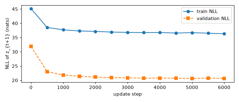
The validation NLL (about 21) is much lower than the training NLL (about 36). The reason for this unusual reversal lies in the inactive dimensions from Chapter 8. The Chapter 8 VAE used only 7 of its 32 dimensions; for the remaining 25, \(q(z_j \mid x) \approx \mathcal{N}(0, 1)\) for every image.
| Split | Input z | NLL of one inactive dimension | Sum over 25 |
| Training | A fresh \(z = \mu + \sigma\epsilon\) is drawn every time. Inactive dimensions carry pure \(\mathcal{N}(0,1)\) noise. | \(\tfrac{1}{2}\log(2\pi e) \approx 1.419\) | About 35.5 |
| Validation | The mean \(\mu\) is used without noise. In inactive dimensions \(\mu\) is nearly constant at 0. | \(\tfrac{1}{2}\log 2\pi + \tfrac{1}{2}\cdot 0^2 \approx 0.919\) | About 23.0 |
- Training: no model can predict pure noise, and the best it can do is predict \(\mathcal{N}(0,1)\) itself. The NLL is then the entropy of the standard normal distribution (Chapter 3), \(\mathbb{E}[-\log\mathcal{N}(z;0,1)] = \tfrac{1}{2}\log 2\pi + \tfrac{1}{2}\mathbb{E}[z^2] = \tfrac{1}{2}\log(2\pi e)\). The 25-dimension sum of 35.5 accounts for almost all of the training NLL of 36.
- Validation: because of the noise seen in training, the model predicts \(\sigma \approx 1\), giving 0.919 per dimension. The remaining 7 active dimensions are predicted well and contribute negative NLL, bringing the total to about 21.
"The NLL won't go below 36" is not a failure of the model; it comes from noise inherent in the data. Loss values should be read against such a floor.
Dreaming: feeding predictions back as input
Once trained, the MDN-RNN can generate the future without the real environment. Given the first frame's \(z\) and an action, it samples the next \(z\), feeds that back as input, samples the next \(z\) again, and so on. This is called a dream or an imagined rollout. Decoding the sampled \(z\) values into images with the Chapter 8 VAE decoder shows what the model is imagining.
@torch.no_grad()
def dream(model, z_real, actions, warmup: int, tau: float):
    """처음 warmup 스텝은 진짜 z 를 넣어 기억(h)을 만들고, 그 뒤로는 자기 예측을 다시 넣는다.

    z_real : (1, T+1, D) 진짜 잠재 시퀀스 (처음 warmup+1 개만 쓴다)
    actions: (1, T, 1) 행동 — 꿈속에서도 진짜와 같은 행동을 넣어 비교한다
    반환    : (T+1, D) 꿈속 z 시퀀스
    """
    state = model.initial_state(1, z_real.device)
    z = z_real[:, 0:1]  # (1, 1, D)
    out = [z[0, 0]]
    for t in range(actions.shape[1]):
        log_pi, mu, log_sigma, _, state = model(z, actions[:, t : t + 1], state)
        if t + 1 <= warmup:
            z = z_real[:, t + 1 : t + 2]  # 아직은 진짜를 보여 준다
        else:
            z = mdn_sample(log_pi, mu, log_sigma, tau)  # 이제부터는 꿈: 자기가 뽑은 z 를 다시 입력
        out.append(z[0, 0])
    return torch.stack(out)
Experimental setup
- For the first 10 steps (
warmup), the real \(z\) is fed in. A single image cannot convey velocity, so a few frames are shown to let the LSTM's memory capture how fast the pendulum is currently turning. After that, the model proceeds using only its own sampled \(z\). - For comparison, the actions are identical to those of the real episode, and validation episodes not used in training are used.
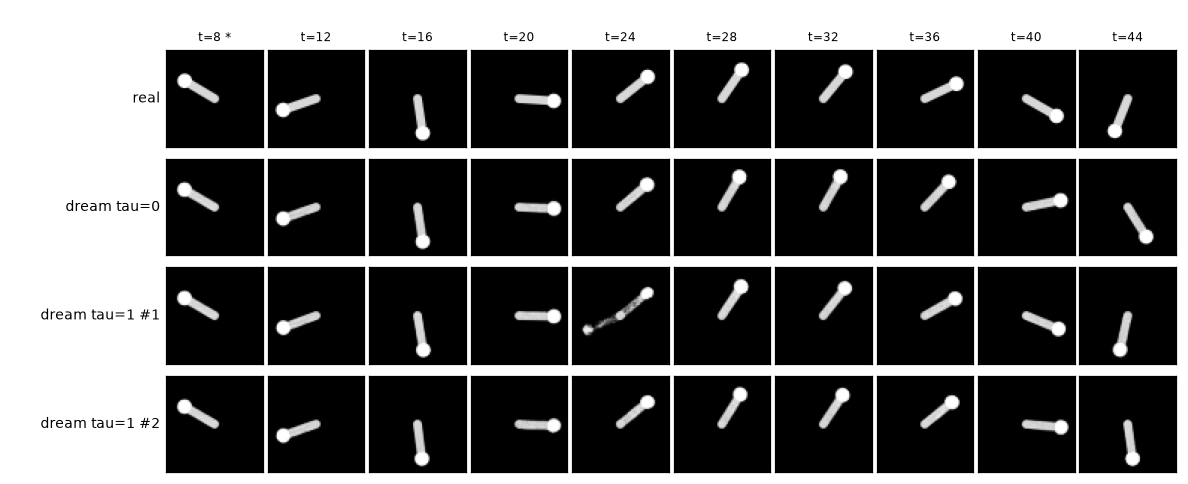
- Figure 9-6 decodes the real episode, one \(\tau = 0\) dream, and two \(\tau = 1\) dreams (same start, different random seeds) and lays them side by side in time order. The span \(t \le 10\) is where real frames were shown.
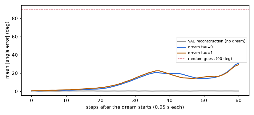
- Figure 9-7 runs dreams on all 20 validation episodes (\(\tau = 1\) four times per episode, 80 dreams in total), reads the angle from each decoded image, and compares it with the real angle. Measurements run up to 60 steps after the dream starts.
- Reading the angle (
image_angle): the brightness-weighted centroid lies on the rod, so the direction from the center toward the centroid is the rod's direction. When the VAE merely reconstructs images without dreaming, the error is around 0.5°, so the error of this reading method is negligible. - Random guessing gives an average error of 90°.
- Figures: Frames of the real episode versus dreams (Figure 9-6), Mean angle error by step after the dream starts (Figure 9-7)
Results
| Steps after the dream starts (time) | Mean angle error |
| 10 (0.5 s) | 1–2° (1° at \(\tau = 0\), 2° at \(\tau = 1\)) |
| 25 (1.25 s) | 7–8° (7° at \(\tau = 0\), 8° at \(\tau = 1\)) |
| Around 35 | About 20° |
| 50 | 14–16° (14° at \(\tau = 0\), 16° at \(\tau = 1\)) |
| 60 | About 30° |
- It learned the physics. Without seeing a single real frame, the error is 1–2° after 10 steps and still 7–8° after 25 steps. In Figure 9-6, from t = 12 to 32 the dreamed pendulum swings at almost the same angle as the real one. Gravity, rotation under torque, and memory of velocity are all captured inside the LSTM.
- It drifts over time. Small prediction errors at each step feed into the next input and accumulate (error accumulation from Chapter 6, exposure bias). The angle error rises and falls with the pendulum's swing rather than growing monotonically. In a system like a pendulum, where small differences grow large, this is unavoidable, but it is still far better than random guessing (90°).
- A \(\tau = 1\) dream is one of many possible futures. Its mean error is almost the same as at \(\tau = 0\), but the two \(\tau = 1\) dreams in Figure 9-6 take different paths from around t = 36 to 40. Occasionally a frame shows a blurred, smeared rod, as at t = 24; this is a moment when the mixture switches components. A \(\tau = 1\) dream does not try to hit a single correct answer but shows one of the futures that could happen, and in Chapter 10 this uncertainty turns out to be useful.
Combining V (the VAE) and M (the MDN-RNN) turns the world of images into a small simulator in a 32-dimensional latent space. Because this simulator does not render images, it is much faster than the real environment, thousands of copies can run at once, and it is differentiable. Chapter 10 learns behavior inside this dream.
Outputs for Chapter 10
| File | Contents |
| | The trained MDN-RNN. Load it with |
| | \(\mu, \log\sigma^2\), actions, and rewards for every episode. Chapter 10 uses them as the starting frames of dreams. |
Summary
- A single image does not capture velocity (partial observability). A hidden state \(h_t\) summarizing past frames is needed.
- An RNN computes \(h_t = \tanh(W_h h_{t-1} + W_x x_t + b)\). The gradient to the distant past is \(\prod\operatorname{diag}(1-h_t^2)W_h\), so it tends to vanish or explode.
- Thanks to the additive path of its cell state, an LSTM preserves gradients with \(\partial c_T/\partial c_k \approx \prod\operatorname{diag}(f_t)\). The GRU is a variant with only two gates. Explosion is prevented with gradient clipping.
- MSE regression outputs the conditional mean. When the future branches, the mean is a future that never happens. A mixture density network keeps every branch with \(\sum_k\pi_k\mathcal{N}(\mu_k,\sigma_k^2)\).
- The mixture log-likelihood is computed safely with log-sum-exp, \(m + \log\sum e^{a_k - m}\). The temperature \(\tau\) controls the randomness of the dream.
- The MDN-RNN predicts a mixture over \(z_{t+1}\) and \(r_t\) from \((z_t, a_t)\). It is trained with teacher forcing, and in dreams it feeds its own predictions back as input.
- The pendulum dream keeps the mean angle error under 8° even 25 steps (1.25 s) in; after that errors accumulate, growing to 15–20° at 35–50 steps and about 30° at 60 steps.
Exercises
- 1. RNN computation
- For a one-dimensional RNN with \(W_h = 1\), \(W_x = 1\), \(b = 0\) and input \(x = (1, 0, 0)\), compute \(h_1, h_2, h_3\) and compare with the example in the text (\(W_h = 0.5\)).
- Answer: \(h_1 = \tanh 1 \approx 0.762\), \(h_2 = \tanh(0.762) \approx 0.642\), \(h_3 = \tanh(0.642) \approx 0.566\). The memory decays much more slowly. However, if \(W_h\) is larger still (e.g., 3), \(h\) sticks near 1 even without input, tanh saturates, \(1 - h^2 \approx 0\), and the gradient vanishes.
- 2. Vanishing gradient
- If the factor multiplied at each step is 0.9, find the scaling of the gradient flowing back 50 steps, and compare it with an LSTM whose forget gate is 0.99.
- Answer: \(0.9^{50} \approx 0.0052\) and \(0.99^{50} \approx 0.605\). With a forget gate close to 1, 60% of the gradient survives even 50 steps back.
- 3. log-sum-exp
- For \(a = (2,\ 0,\ -1)\), compute \(\log\sum e^{a_k}\) with the stabilized formula (\(e^{-2} \approx 0.135\), \(e^{-3} \approx 0.050\)).
- Answer: \(m = 2\), so \(2 + \log(e^0 + e^{-2} + e^{-3}) = 2 + \log(1.185) \approx 2 + 0.170 = 2.170\).
- 4. Temperature
- For \(\pi = (0.5,\ 0.3,\ 0.2)\), find the component selection probabilities as \(\tau \to 0\) and \(\tau \to \infty\).
- Answer: as \(\tau \to 0\), only the largest value 0.5 survives in \(\pi_k^{1/\tau}\), giving \((1, 0, 0)\). As \(\tau \to \infty\), \(\pi_k^{1/\tau} \to \pi_k^0 = 1\), giving the uniform \((1/3, 1/3, 1/3)\).
- 5. The NLL floor
- If the Chapter 8 VAE had used only 3 active dimensions instead of 7, find the lower limit of the training NLL (assume the active dimensions contribute 0).
- Answer: 29 inactive dimensions × 1.419 ≈ 41.1. The training NLL cannot drop below about 41.
See also
- World Models:Tutorial
- World Models
- Recurrent World Models Facilitate Policy Evolution
- Recurrent neural network
- LSTM
- GRU
- Backpropagation through time
- Gradient Vanishing
- Gradient Exploding
- Mixture Density Network
- Gaussian mixture model
- Maximum likelihood estimation
- VAE