WorldModels:Tutorial:08-VAE
lastmod 2026-11-18created 2026-11-172 edits
Building the Eyes: VAE is chapter 8 of the World Model tutorial. The World Model in chapters 6 and 7 received the pendulum's state as three numbers \([\cos\theta, \sin\theta, \dot\theta]\), but from this chapter on the agent sees only a 64×64 grayscale image. Instead of predicting the image directly, we first build eyes that compress it into 32 numbers: a variational autoencoder (VAE). The chapter covers latent variable models, two derivations of the ELBO, the closed form of the KL term, the choice of decoder likelihood, the reparameterization trick, a convolutional implementation, and experimental results. The VAE and episode data trained here are reused in chapters 9 and 10.
- Original: 08. Building the Eyes: VAE
- Code:
code/ch08_vae.py,code/wm_envs.py(2–4 minutes in total on a laptop GPU, about 50 minutes on 4 CPU threads;--quickfinishes in under a minute on CPU) - Previous: 07. MPC and CEM / Next: 09. RNN and MDN-RNN
Why compress images
An observation \(o_t\) in the PixelPendulum environment has 64×64 = 4096 pixels, each with a brightness from 0 to 255. A World Model's job is to look at the current image and action and predict the next image, but predicting all 4096 numbers at once is hard and wasteful.
- Most pixels are always 0 (black). The rod covers only a few hundred pixels.
- The image can change in only one way. A pendulum image is fully determined by a single angle \(\theta\), so all such images lie on a thin loop in 4096-dimensional space that goes around once as the angle changes.
- 4096 pixels with 256 levels each can form \(256^{4096}\) images, but pendulum images make up just a one-dimensional loop among them.
The idea that high-dimensional data actually lies on a surface or curve of much lower dimension is called the manifold hypothesis. We can convert an image into coordinates on that curve, make predictions in coordinate space, and turn coordinates back into images only when needed. This is the strategy of Ha & Schmidhuber's (2018) World Models (chapter 10), and the VAE in this chapter corresponds to the V (Vision, the eyes) in that architecture.
The overall pipeline is image \(x\) (64×64 = 4096) → encoder \(q_\phi(z \mid x)\) → latent vector \(z\) (32 numbers) → decoder \(p_\theta(x \mid z)\) → reconstruction \(\hat{x}\) (64×64). The middle is a bottleneck that narrows from 4096 → 32 → 4096.
Autoencoders and their limits
The simplest compressor is an autoencoder (AE). The encoder \(f_\phi\) shrinks an image \(x\) into a small vector \(z = f_\phi(x)\), and the decoder \(g_\theta\) restores it as \(\hat{x} = g_\theta(z)\). Because the target is the input itself, no human labeling is needed (self-supervised learning), and because \(z\) is much smaller than the input, it ends up holding only the information essential for restoring the image.
\(\min_{\phi,\theta}\; \frac{1}{N}\sum_{n=1}^{N} \text{재구성 오차}\big(x^{(n)},\; g_\theta(f_\phi(x^{(n)}))\big)\)
The reconstruction error is usually per-pixel squared error (MSE) or binary cross-entropy (BCE). Autoencoders reconstruct well. The problem is the shape of the latent space. This chapter's code also trains an autoencoder with the same architecture as the VAE for comparison, and two problems show up.
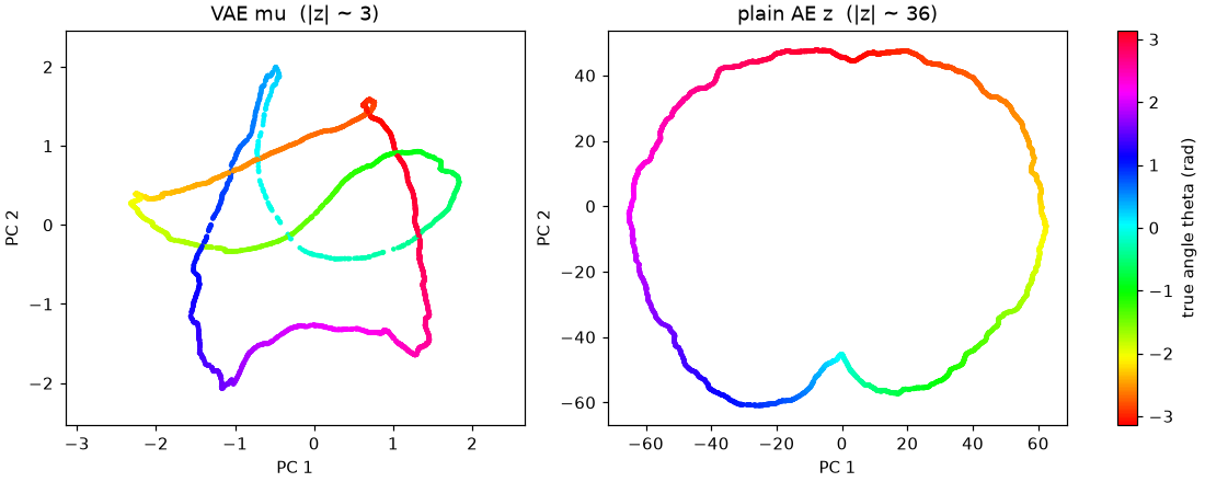
- We don't know where the latent vectors are. There is no constraint on the range of \(z\). In the trained autoencoder, a single component of \(z\) reached magnitudes of up to 36, and measured along principal axes the vectors spread out to around ±60. To generate a new image, we have no idea where to sample \(z\) from.
- The latent space is sparse. The decoder is trained only on the points where the training data actually lands. Feed it a \(z\) between or outside those points and it gets an input it has never seen, producing a nonsensical image.
The M model in chapter 9 imagines the future by sampling the next \(z\) in latent space, so if a sampled \(z\) lands somewhere the decoder doesn't know, the imagination immediately falls apart. What we need is a latent space where we know the distribution \(z\) follows, and where any \(z\) drawn from that distribution decodes to a plausible image. The VAE solves this with a probabilistic model.
Latent variable models
Generative process and marginal likelihood
A VAE assumes images are generated as follows.
- Sample a latent vector from the standard normal distribution: \(z \sim p(z) = \mathcal{N}(0, I)\) (32 independent components, each with mean 0 and variance 1).
- Feed \(z\) into the decoder to define a distribution over images, and sample an image from it: \(x \sim p_\theta(x \mid z)\).
Since \(z\) is not directly visible in the data, it is called a latent variable. The probability of a single image (the marginal likelihood) is obtained by marginalizing the joint probability over \(z\) and applying the product rule \(p(x, z) = p(x \mid z)\,p(z)\).
\(p_\theta(x) = \int p_\theta(x, z)\, dz = \int p_\theta(x \mid z)\, p(z)\, dz\)
The training objective is maximum likelihood (chapter 2).
\(\theta^\ast = \operatorname*{arg\,max}_\theta \sum_{n=1}^{N} \log p_\theta\big(x^{(n)}\big)\)
Why it cannot be computed
Since \(z\) is 32-dimensional, the integral above is a 32-fold integral. Even dividing each axis into just 10 cells means running the decoder on \(10^{32}\) cells. A Monte Carlo estimate that samples \(z\) from the prior and averages is correct as a formula.
\(p_\theta(x) = \mathbb{E}_{z \sim p(z)}\big[p_\theta(x \mid z)\big] \approx \frac{1}{S}\sum_{s=1}^{S} p_\theta\big(x \mid z^{(s)}\big),\qquad z^{(s)} \sim p(z)\)
However, only a tiny region of the latent space produces a particular image \(x\). For a randomly drawn \(z\), \(p_\theta(x \mid z^{(s)})\) is effectively 0, and the rare sample that happens to land in that region dominates the average. The estimate's variance is too large to serve as a training signal.
The posterior \(p_\theta(z \mid x)\) answers where the \(z\) that produced \(x\) is likely to be, and it can be written using Bayes' theorem.
\(p_\theta(z \mid x) = \frac{p_\theta(x \mid z)\, p(z)}{p_\theta(x)} = \frac{p_\theta(x \mid z)\, p(z)}{\int p_\theta(x \mid z')\, p(z')\, dz'}\)
The numerator takes a single decoder pass, but the denominator is exactly the integral we cannot compute. When neither \(p_\theta(x)\) nor \(p_\theta(z \mid x)\) can be computed, the posterior is said to be intractable.
Variational inference: a neural network that guesses the posterior
Variational inference replaces the intractable \(p_\theta(z \mid x)\) with an approximation by a tractable distribution \(q_\phi(z \mid x)\). A VAE builds this \(q_\phi\) as a neural network (the encoder).
\(q_\phi(z \mid x) = \mathcal{N}\big(z;\ \mu_\phi(x),\ \operatorname{diag}(\sigma^2_\phi(x))\big)\)
- The encoder takes an image \(x\) and outputs 32 means \(\mu_\phi(x)\) and 32 variances \(\sigma^2_\phi(x)\). This is a guess that the \(z\) that produced the image is near \(\mu\), with an error of about \(\sigma\).
- \(\operatorname{diag}(\cdot)\) means a diagonal covariance, i.e. a Gaussian whose 32 components are independent. It is simple but cheap to compute.
- The actual output is \(\log \sigma^2\), not \(\sigma^2\). A neural network can output negative numbers but variance must be positive, so converting with \(\sigma = \exp(\tfrac{1}{2}\log\sigma^2)\) always gives a positive value. Whether \(\sigma\) is 0.001 or 100, \(\log\sigma\) is −6.9 or 4.6 (−13.8 and 9.2 as log variance), so the numeric range is also narrow.
Instead of solving a separate optimization problem for each image, a single network outputs \(q\) for every image at once, which is why this is also called amortized inference. The ELBO answers the question of what to maximize so that \(q_\phi\) becomes a good guess while \(p_\theta(x)\) also grows.
ELBO
Derivation 1: Jensen's inequality
A concave function such as the logarithm satisfies Jensen's inequality \(\log \mathbb{E}[Y] \ge \mathbb{E}[\log Y]\) (chapter 3). For example, if \(Y\) is 1 or 4 with equal probability, then \(\log \mathbb{E}[Y] = \log 2.5 \approx 0.916\) and \(\mathbb{E}[\log Y] = \tfrac{1}{2}(\log 1 + \log 4) \approx 0.693\). We multiply inside the integral by \(q_\phi / q_\phi = 1\) to turn it into an expectation, then apply the inequality.
\(\begin{align} \log p_\theta(x) &= \log \int p_\theta(x, z)\, dz \\ &= \log \int q_\phi(z \mid x)\, \frac{p_\theta(x, z)}{q_\phi(z \mid x)}\, dz \\ &= \log \mathbb{E}_{z \sim q_\phi(z \mid x)}\left[\frac{p_\theta(x, z)}{q_\phi(z \mid x)}\right] \\ &\ge \mathbb{E}_{z \sim q_\phi(z \mid x)}\left[\log \frac{p_\theta(x, z)}{q_\phi(z \mid x)}\right] \\ &= \mathbb{E}_{q_\phi}\left[\log p_\theta(x \mid z) + \log p(z) - \log q_\phi(z \mid x)\right] \\ &= \mathbb{E}_{q_\phi}\left[\log p_\theta(x \mid z)\right] - \mathbb{E}_{q_\phi}\left[\log q_\phi(z \mid x) - \log p(z)\right] \end{align}\)
The equality becomes an inequality on the fourth line. The second term on the last line is exactly the definition of the KL divergence, \(D_{\mathrm{KL}}(q\,\Vert\,p) = \mathbb{E}_q[\log q - \log p]\).
\(\log p_\theta(x) \;\ge\; \underbrace{\mathbb{E}_{q_\phi(z \mid x)}\left[\log p_\theta(x \mid z)\right] - D_{\mathrm{KL}}\big(q_\phi(z \mid x)\,\Vert\,p(z)\big)}_{\text{ELBO}(\theta,\phi;\,x)}\)
The right-hand side is the ELBO (Evidence Lower BOund). The evidence is another name for \(p_\theta(x)\). Both terms can be computed. The first term just requires sampling \(z\) from \(q_\phi\) and feeding it to the decoder, and the second is a KL between two Gaussians, which has a formula. Training a VAE means maximizing this computable lower bound in place of the intractable \(\log p_\theta(x)\).
Derivation 2: what the gap is
Jensen's inequality only tells us that the ELBO is less than \(\log p_\theta(x)\). How much less can be derived purely with equalities, starting from the KL between the approximation \(q_\phi(z \mid x)\) and the true posterior \(p_\theta(z \mid x)\). Substitute the log of Bayes' theorem, \(\log p_\theta(z \mid x) = \log p_\theta(x, z) - \log p_\theta(x)\), and pull the constant \(\log p_\theta(x)\), which does not depend on \(z\), out of the expectation.
\(\begin{align} D_{\mathrm{KL}}\big(q_\phi(z \mid x)\,\Vert\,p_\theta(z \mid x)\big) &= \mathbb{E}_{q_\phi}\left[\log q_\phi(z \mid x) - \log p_\theta(z \mid x)\right] \\ &= \mathbb{E}_{q_\phi}\left[\log q_\phi(z \mid x) - \log p_\theta(x, z) + \log p_\theta(x)\right] \\ &= \mathbb{E}_{q_\phi}\left[\log q_\phi(z \mid x) - \log p_\theta(x, z)\right] + \log p_\theta(x) \\ &= -\,\mathbb{E}_{q_\phi}\left[\log \frac{p_\theta(x, z)}{q_\phi(z \mid x)}\right] + \log p_\theta(x) \\ &= -\,\text{ELBO} + \log p_\theta(x) \end{align}\)
\(\log p_\theta(x) = \text{ELBO}(\theta, \phi; x) + D_{\mathrm{KL}}\big(q_\phi(z \mid x)\,\Vert\,p_\theta(z \mid x)\big)\)
The log-likelihood (not computable) splits exactly into the ELBO (computable) plus the approximation error (KL ≥ 0). Several things follow from this identity.
- Since KL ≥ 0, ELBO ≤ \(\log p_\theta(x)\). Equality holds only when \(q_\phi(z \mid x) = p_\theta(z \mid x)\).
- Raising the ELBO with respect to the encoder \(\phi\) shrinks the gap. Since \(\log p_\theta(x)\) is fixed and independent of \(\phi\), the KL decreases by as much as the ELBO increases, and the encoder moves closer to the true posterior.
- Raising the ELBO with respect to the decoder \(\theta\) generally raises \(\log p_\theta(x)\). Pushing up a lower bound pushes up the value above it.
A VAE maximizes a single objective, the ELBO, with respect to \(\phi\) and \(\theta\) simultaneously. As a loss function, it minimizes the negated −ELBO.
The roles of the two terms
\(\text{ELBO} = \underbrace{\mathbb{E}_{q_\phi(z \mid x)}\big[\log p_\theta(x \mid z)\big]}_{\text{(1) 재구성 항}} \;-\; \underbrace{D_{\mathrm{KL}}\big(q_\phi(z \mid x)\,\Vert\,p(z)\big)}_{\text{(2) KL 항 (정규화)}}\)
- Reconstruction term
- The log probability that the original image \(x\) comes out when a \(z\) sampled from the encoder's guess is fed to the decoder. Higher is better. It plays the same role as an autoencoder's reconstruction error.
- KL term
- Keeps each image's guess \(q_\phi(z \mid x)\) from drifting too far from the prior \(\mathcal{N}(0, I)\). Lower is better.
The original tutorial uses a library analogy. When a librarian (the encoder) assigns a shelf location (\(z\)) to each book (image), the reconstruction term is the rule that the book must be findable again from its location alone, and the KL term is the rule that locations must be packed into a designated area near the entrance (\(\mathcal{N}(0, I)\)) and given as a range rather than a single point.
The KL term solves the autoencoder's two problems as follows.
- We know where to sample from. Since every image's \(q_\phi(z \mid x)\) gathers near the origin with a scale of about 1, we can expect the overall \(z\) to roughly follow \(\mathcal{N}(0, I)\). New images are generated by sampling \(z\) from \(\mathcal{N}(0, I)\).
- The latent space becomes dense. The encoder outputs a cloud of width \(\sigma\) rather than a point, and during training any point within that cloud is sampled and fed to the decoder. The decoder learns to produce the same image across that whole neighborhood, so nearby \(z\) values give similar images. As the clouds are pulled toward the origin and overlap, gaps also shrink. Because \(-\log\sigma^2\) grows without bound as \(\sigma \to 0\), the KL term also prevents the clouds from collapsing to points.
The two terms are in a tug-of-war. Looking only at reconstruction, it pays to make the clouds very small and far apart (an autoencoder); looking only at KL, it pays to send every image to the same \(\mathcal{N}(0, I)\) (then \(z\) carries no information and reconstruction is impossible). A VAE finds the balance between them.
Closed form of the KL term
One dimension
For \(q = \mathcal{N}(\mu, \sigma^2)\) and \(p = \mathcal{N}(0, 1)\), the two log densities are as follows.
\(\log q(z) = -\tfrac{1}{2}\log(2\pi) - \tfrac{1}{2}\log\sigma^2 - \frac{(z - \mu)^2}{2\sigma^2},\qquad \log p(z) = -\tfrac{1}{2}\log(2\pi) - \frac{z^2}{2}\)
Subtracting cancels the common term \(-\tfrac{1}{2}\log 2\pi\). Then plug in \(\mathbb{E}_q\big[(z-\mu)^2\big] = \sigma^2\) and \(\mathbb{E}_q\big[z^2\big] = \operatorname{Var}(z) + (\mathbb{E}[z])^2 = \sigma^2 + \mu^2\).
\(\begin{align} D_{\mathrm{KL}}(q\,\Vert\,p) &= \mathbb{E}_{z \sim q}\left[-\tfrac{1}{2}\log\sigma^2 - \frac{(z - \mu)^2}{2\sigma^2} + \frac{z^2}{2}\right] \\ &= -\tfrac{1}{2}\log\sigma^2 - \frac{\sigma^2}{2\sigma^2} + \frac{\sigma^2 + \mu^2}{2} \\ &= \tfrac{1}{2}\big(\mu^2 + \sigma^2 - 1 - \log\sigma^2\big) \end{align}\)
With \(\mu = 0,\ \sigma = 1\) this is 0, matching the requirement that the KL between identical distributions is 0. \(\mu^2\) is a penalty that grows as the mean moves away from 0, and \(\sigma^2 - 1 - \log\sigma^2\) is a penalty that grows as \(\sigma\) moves away from 1. For \(g(s) = s - 1 - \log s\) (\(s = \sigma^2\)), \(g'(s) = 1 - \tfrac{1}{s}\), so \(g\) decreases for \(s \lt 1\), increases for \(s \gt 1\), and has its minimum \(g(1) = 0\) at \(s = 1\). This term is always non-negative and is 0 only when \(\sigma = 1\).
32 dimensions
A Gaussian with diagonal covariance has independent components, so its density is the product of per-component densities (\(q_j = \mathcal{N}(\mu_j, \sigma_j^2)\), \(p_j = \mathcal{N}(0, 1)\)). The log of a product is the sum of logs, and since the \(j\)-th term depends only on \(z_j\), the integrals over the other components equal 1 and drop out. The KL of a diagonal Gaussian is the sum of the per-dimension KLs.
\(D_{\mathrm{KL}}(q\,\Vert\,p) = \sum_{j=1}^{32} \mathbb{E}_{z_j \sim q_j}\big[\log q_j(z_j) - \log p_j(z_j)\big]\)
\(D_{\mathrm{KL}}\big(q_\phi(z \mid x)\,\Vert\,\mathcal{N}(0, I)\big) = \frac{1}{2}\sum_{j=1}^{32}\big(\mu_j^2 + \sigma_j^2 - 1 - \log\sigma_j^2\big)\)
As a numeric example in 2 dimensions, with \(\mu = (0.5,\ 0)\) and \(\sigma = (1,\ 0.5)\), we get \(\tfrac{1}{2}(0.25 + 1 - 1 - 0) + \tfrac{1}{2}(0 + 0.25 - 1 - \log 0.25) = 0.125 + 0.318 = 0.443\). Here is code that checks this with Monte Carlo, along with its output.
import torch

mu = torch.tensor([0.5, 0.0])
sigma = torch.tensor([1.0, 0.5])

# 닫힌 꼴: ½ Σ (μ² + σ² − 1 − log σ²)
closed = 0.5 * torch.sum(mu**2 + sigma**2 - 1 - torch.log(sigma**2))

# 몬테카를로: z ~ q 를 많이 뽑아 log q(z) − log p(z) 를 평균
q = torch.distributions.Normal(mu, sigma)
p = torch.distributions.Normal(torch.zeros(2), torch.ones(2))
z = q.sample((1_000_000,))
mc = (q.log_prob(z) - p.log_prob(z)).sum(-1).mean()

print(f"닫힌 꼴 {closed.item():.4f} | 몬테카를로 {mc.item():.4f}")
Reconstruction term: the decoder likelihood
To compute the reconstruction term \(\mathbb{E}_{q_\phi}[\log p_\theta(x \mid z)]\), we need to decide how to compute the expectation and what distribution \(p_\theta(x \mid z)\) is.
Estimating the expectation with one sample
We sample a single \(z\) from \(q_\phi(z \mid x)\) and use \(\log p_\theta(x \mid z^{(1)})\) in place of the expectation (\(S = 1\) Monte Carlo). A single sample is noisy but unbiased, and since it is averaged over minibatches of 128 images across thousands of updates, the noise averages out. Monte Carlo, useless when sampling from the prior, works here because \(z\) is drawn from \(q_\phi(z \mid x)\), a guess made after looking at \(x\). Most samples land in the region that produces \(x\) well.
Bernoulli decoder and BCE
A pendulum image is mostly black (0), with a light gray rod (0.85) and a white bob at the end (1). We treat the brightness \(x_i \in [0, 1]\) of pixel \(i\) as a Bernoulli variable with probability \(p_i\) of being white. The decoder outputs a logit \(\ell_i\) for each pixel, with \(p_i = \text{sigmoid}(\ell_i) = \frac{1}{1 + e^{-\ell_i}}\). Given \(z\), pixels are assumed independent.
\(\begin{align} p_\theta(x \mid z) &= \prod_{i=1}^{4096} p_i^{\,x_i}\,(1 - p_i)^{\,1 - x_i} \\ \log p_\theta(x \mid z) &= \sum_{i=1}^{4096}\Big(x_i \log p_i + (1 - x_i)\log(1 - p_i)\Big) \\ -\log p_\theta(x \mid z) &= \sum_{i=1}^{4096} \text{BCE}(x_i, p_i),\qquad \text{BCE}(x, p) = -\big(x\log p + (1-x)\log(1-p)\big) \end{align}\)
The negative log-likelihood is the sum of per-pixel binary cross-entropies (Cross entropy), so the reconstruction loss in the code is binary_cross_entropy_with_logits(..., reduction="sum").
Caveat: gray pixels and the BCE floor. The rod body has brightness 0.85 and its edges are anti-aliased, so there are many gray pixels between 0 and 1. Strictly speaking this is not Bernoulli, but it is common in practice. The catch is that BCE cannot reach 0. For a target \(x \in (0, 1)\), the derivative of \(\text{BCE}(x, p)\) with respect to \(p\) is \(-\frac{x}{p} + \frac{1 - x}{1 - p}\), which is 0 at \(p = x\). The value there, \(-\big(x\log x + (1-x)\log(1-x)\big)\), is the entropy of the pixel. So even if the decoder matches the target exactly, a BCE equal to the sum of the gray pixels' entropies remains for each image. The floor computed by the code was about 80 nats per image (output 79.9), roughly half from the 0.85-brightness rod body and the rest from gray pixels at the edges.
Gaussian decoder and MSE
For natural images with many colors, pixel values are sometimes modeled as a Gaussian with the decoder output \(\hat{x}_i\) as the mean and a fixed variance \(s^2\). Ha & Schmidhuber used this approach (MSE). Here \(D = 4096\).
\(\log p_\theta(x \mid z) = \sum_{i=1}^{D}\log \mathcal{N}(x_i;\ \hat{x}_i,\ s^2) = \sum_{i=1}^{D}\left(-\tfrac{1}{2}\log(2\pi s^2) - \frac{(x_i - \hat{x}_i)^2}{2s^2}\right)\)
\(-\log p_\theta(x \mid z) = \frac{1}{2s^2}\,\lVert x - \hat{x}\rVert^2 + \frac{D}{2}\log(2\pi s^2)\)
The second term is a constant independent of \(\theta\) and does not affect training; what remains is the sum of squared errors multiplied by \(\frac{1}{2s^2}\). \(s\) sets the weight ratio relative to the KL term (see β-VAE below).
The reparameterization trick
Maximizing the ELBO with gradient descent requires gradients with respect to \(\phi\). But in the reconstruction term \(\mathbb{E}_{z \sim q_\phi}[\log p_\theta(x \mid z)]\), \(\phi\) is hidden in which distribution \(z\) is drawn from. A sampling step like z = torch.normal(mu, sigma) does not define how \(z\) changes when \(\mu\) changes slightly, so it cannot be differentiated and backpropagation stops at that line.
For a Gaussian, scaling and shifting a standard normal sample \(\epsilon\) gives a sample from the desired Gaussian.
\(z \sim \mathcal{N}(\mu, \sigma^2) \quad\Longleftrightarrow\quad z = \mu + \sigma\,\epsilon,\quad \epsilon \sim \mathcal{N}(0, 1)\)
\(\mathbb{E}[\mu + \sigma\epsilon] = \mu\), \(\operatorname{Var}(\mu + \sigma\epsilon) = \sigma^2\), and a scaled and shifted Gaussian is still Gaussian. The randomness remains only in \(\epsilon\), which is independent of \(\phi\), and \(z\) becomes a differentiable function of \(\mu, \sigma\). This is the reparameterization trick (Kingma & Welling, 2014). In terms of the computation graph, before reparameterization the gradient stops at the sampling node in \(\mu, \sigma\) → sample (\(z \sim \mathcal{N}\)) → \(f(z)\); after reparameterization, the gradient flows to \(\mu, \sigma\) through the node \(\mu + \sigma\epsilon\), with \(\epsilon\) entering from the side.
Since the distribution over which the expectation is taken no longer depends on \(\mu, \sigma\), differentiation and expectation can be swapped, and by the chain rule \(\frac{\partial z}{\partial \mu} = 1\), \(\frac{\partial z}{\partial \sigma} = \epsilon\).
\(\begin{align} \mathbb{E}_{z \sim \mathcal{N}(\mu,\sigma^2)}\big[f(z)\big] &= \mathbb{E}_{\epsilon \sim \mathcal{N}(0,1)}\big[f(\mu + \sigma\epsilon)\big] \\ \frac{\partial}{\partial \mu}\mathbb{E}_{\epsilon}\big[f(\mu + \sigma\epsilon)\big] &= \mathbb{E}_{\epsilon}\big[f'(\mu + \sigma\epsilon)\cdot 1\big] \\ \frac{\partial}{\partial \sigma}\mathbb{E}_\epsilon\big[f(\mu+\sigma\epsilon)\big] &= \mathbb{E}_{\epsilon}\big[f'(\mu + \sigma\epsilon)\cdot \epsilon\big] \end{align}\)
\(\nabla_{\mu,\sigma}\,\mathbb{E}\big[f(z)\big] \approx \frac{1}{S}\sum_{s=1}^{S} \nabla_{\mu,\sigma} f\big(\mu + \sigma\epsilon^{(s)}\big),\qquad \epsilon^{(s)} \sim \mathcal{N}(0,1)\)
The gradient for each sample is computed by PyTorch's automatic differentiation. To check with \(f(z) = z^2\): \(\mathbb{E}[z^2] = \mu^2 + \sigma^2\), so the true gradients are \(2\mu\) and \(2\sigma\), and the formula gives the same, \(\mathbb{E}_\epsilon[2(\mu + \sigma\epsilon)] = 2\mu\) and \(\mathbb{E}_\epsilon[2(\mu+\sigma\epsilon)\epsilon] = 2\mu\mathbb{E}[\epsilon] + 2\sigma\mathbb{E}[\epsilon^2] = 2\sigma\). The code below parameterizes by \(\log\sigma\) as a VAE does, so the correct answer is \(\frac{\partial}{\partial \log\sigma}(\mu^2 + \sigma^2) = 2\sigma\cdot\sigma = 2\sigma^2\).
import torch

torch.manual_seed(0)
mu = torch.tensor(1.5, requires_grad=True)
log_sigma = torch.tensor(0.0, requires_grad=True)   # σ = e^0 = 1

eps = torch.randn(100_000)                  # ε ~ N(0, 1): μ, σ 와 상관없는 잡음
z = mu + log_sigma.exp() * eps              # z = μ + σ ε  ← 미분이 지나가는 길
loss = (z ** 2).mean()                      # E[z²] 의 몬테카를로 추정
loss.backward()

print(f"E[z^2] 추정  {loss.item():.3f}   (정답 μ²+σ² = {1.5**2 + 1:.3f})")
print(f"dE/dμ 추정   {mu.grad.item():.3f}   (정답 2μ = {2*1.5:.3f})")
print(f"dE/dlogσ 추정 {log_sigma.grad.item():.3f}   (정답 2σ² = {2*1.0:.3f})")
E[z^2] 추정  3.245   (정답 μ²+σ² = 3.250)
dE/dμ 추정   2.995   (정답 2μ = 3.000)
dE/dlogσ 추정 1.998   (정답 2σ² = 2.000)
When a distribution cannot be reparameterized (for example, a discrete choice), the score-function (REINFORCE) estimator \(\nabla_\phi\mathbb{E}_{q_\phi}[f(z)] = \mathbb{E}_{q_\phi}[f(z)\,\nabla_\phi\log q_\phi(z)]\) is used. It is the same formula as the policy gradient in chapter 5. It works for any distribution but has much higher variance, so reparameterization is preferred whenever possible. Dreamer in chapter 12 uses both methods.
Implementation: a convolutional VAE
Data
The pendulum is driven with random torque (uniform on \([-2, 2]\)) for 200 episodes, collecting 40,200 images (collect_pixel_episodes, region collect). Since starting angles are uniformly random, images of every angle are evenly represented. The returned arrays are obs (N, T+1, 64, 64) uint8, action (N, T, 1), reward (N, T), and state (N, T+1, 3). The ground-truth state is used only to check what the VAE has learned, never for training.
Computing output sizes
The encoder shrinks the image through four convolutions with kernel size 4 and stride 2, and the decoder enlarges it again with transposed convolutions. This is Ha & Schmidhuber's architecture adapted to a single grayscale channel.
\(\text{합성곱: } W_{\text{out}} = \left\lfloor \frac{W_{\text{in}} + 2P - K}{S} \right\rfloor + 1,\qquad \text{전치 합성곱: } W_{\text{out}} = (W_{\text{in}} - 1)\,S - 2P + K\)
- The convolution formula counts how many positions a window of size \(K\) can occupy when it moves \(S\) cells at a time across an input padded by \(P\) on each side.
- In a transposed convolution, each input cell stamps a pattern of size \(K\) onto the output, and neighboring input cells stamp \(S\) cells apart. From the resulting length \((W_{\text{in}}-1)S + K\), padding \(P\) is trimmed from both sides. This is the same as solving the convolution formula backward for \(W_{\text{in}}\).
- Encoder (\(K = 4,\ S = 2,\ P = 0\)): \(64 \to 31 \to 14 \to 6 \to 2\). \(\tfrac{27}{2} = 13.5\) is rounded down to 13. At the end, 256 channels × 2 × 2 = 1024 numbers remain.
- Decoder: \(z\) is expanded to 1024 numbers, treated as a 1×1 image with 1024 channels, and transposed convolutions with kernel sizes 5, 5, 6, 6 and stride 2 produce \(1 \to 5 \to 13 \to 30 \to 64\).
| Layer | Configuration | Output shape (channels, height, width) | Parameters |
| Input | Grayscale image | (1, 64, 64) | None |
| Conv 1 | 32 channels, 4×4, stride 2, ReLU | (32, 31, 31) | 1·32·16 + 32 = 544 |
| Conv 2 | 64 channels, 4×4, stride 2, ReLU | (64, 14, 14) | 32·64·16 + 64 = 32,832 |
| Conv 3 | 128 channels, 4×4, stride 2, ReLU | (128, 6, 6) | 64·128·16 + 128 = 131,200 |
| Conv 4 | 256 channels, 4×4, stride 2, ReLU | (256, 2, 2) → flattened to 1024 | 128·256·16 + 256 = 524,544 |
| μ, log σ² | Fully connected 1024 → 32 (two of them) | (32), (32) | 2 × (1024·32 + 32) = 65,600 |
| Decoder input | Fully connected 32 → 1024 | (1024, 1, 1) | 32·1024 + 1024 = 33,792 |
| Transposed conv 1 | 128 channels, 5×5, stride 2, ReLU | (128, 5, 5) | 1024·128·25 + 128 = 3,276,928 |
| Transposed conv 2 | 64 channels, 5×5, stride 2, ReLU | (64, 13, 13) | 128·64·25 + 64 = 204,864 |
| Transposed conv 3 | 32 channels, 6×6, stride 2, ReLU | (32, 30, 30) | 64·32·36 + 32 = 73,760 |
| Transposed conv 4 | 1 channel, 6×6, stride 2 (logits) | (1, 64, 64) | 32·1·36 + 1 = 1,153 |
The parameter count of a convolutional layer is input channels × output channels × kernel size + output channels (biases). The total is about 4.35 million, and 75% of it is concentrated in the decoder's first transposed convolution.
Model
class ConvVAE(nn.Module):
    """합성곱 VAE. 입력 (B, 1, 64, 64) 값 범위 [0, 1] → 잠재 z (B, z_dim)."""

    def __init__(self, z_dim: int = 32):
        super().__init__()
        self.z_dim = z_dim
        # 인코더: 4×4 합성곱, 보폭 2 를 네 번. 64 → 31 → 14 → 6 → 2
        self.enc = nn.Sequential(
            nn.Conv2d(1, 32, 4, stride=2), nn.ReLU(),  # (B, 32, 31, 31)
            nn.Conv2d(32, 64, 4, stride=2), nn.ReLU(),  # (B, 64, 14, 14)
            nn.Conv2d(64, 128, 4, stride=2), nn.ReLU(),  # (B, 128, 6, 6)
            nn.Conv2d(128, 256, 4, stride=2), nn.ReLU(),  # (B, 256, 2, 2)
            nn.Flatten(),  # (B, 1024)
        )
        self.fc_mu = nn.Linear(1024, z_dim)  # 평균 μ
        self.fc_logvar = nn.Linear(1024, z_dim)  # 로그 분산 log σ²
        # 디코더: z → 1024 → (1024, 1, 1) 에서 전치 합성곱으로 1 → 5 → 13 → 30 → 64
        self.fc_dec = nn.Linear(z_dim, 1024)
        self.dec = nn.Sequential(
            nn.ConvTranspose2d(1024, 128, 5, stride=2), nn.ReLU(),  # (B, 128, 5, 5)
            nn.ConvTranspose2d(128, 64, 5, stride=2), nn.ReLU(),  # (B, 64, 13, 13)
            nn.ConvTranspose2d(64, 32, 6, stride=2), nn.ReLU(),  # (B, 32, 30, 30)
            nn.ConvTranspose2d(32, 1, 6, stride=2),  # (B, 1, 64, 64) 로짓
        )

    def encode(self, x):
        """q_φ(z|x) 의 평균과 로그 분산."""
        h = self.enc(x)
        return self.fc_mu(h), self.fc_logvar(h)

    def reparameterize(self, mu, logvar):
        """재매개변수화: z = μ + σ ⊙ ε,  ε ~ N(0, I)."""
        std = torch.exp(0.5 * logvar)  # σ = exp(½ log σ²)
        eps = torch.randn_like(std)
        return mu + std * eps

    def decode_logits(self, z):
        """p_θ(x|z) 의 베르누이 로짓. 픽셀 밝기 = sigmoid(로짓)."""
        h = self.fc_dec(z).view(-1, 1024, 1, 1)
        return self.dec(h)

    def decode(self, z):
        return torch.sigmoid(self.decode_logits(z))

    def forward(self, x):
        mu, logvar = self.encode(x)
        z = self.reparameterize(mu, logvar)
        return self.decode_logits(z), mu, logvar
-
fc_muandfc_logvarproduce two 32-dimensional vectors from the same 1024 features: the \(\mu\) and \(\log\sigma^2\) of \(q_\phi(z \mid x)\). -
reparameterizecomputes \(\sigma = \exp(\tfrac{1}{2}\log\sigma^2) = (\sigma^2)^{1/2}\) and \(z = \mu + \sigma\odot\epsilon\).randn_likesamples an \(\epsilon\) of the same shape. -
decode_logitsreturns logits, not brightness values. The sigmoid is computed inside the loss function. -
forward(encode → reparameterize → decode) is the path used during training. When chapter 10 converts images from the real environment into \(z\), it uses the mean \(\mu\) without sampling. When training the MDN-RNN in chapter 9, a fresh \(z\) is sampled for each batch from the stored \(\mu, \log\sigma^2\). - The
ConvAEused for comparison has the same architecture with only the probabilistic parts (\(\sigma\), KL) removed, and is trained on the BCE sum alone.
Loss function
def vae_loss(logits, x, mu, logvar, beta: float = 1.0):
    """음의 ELBO (그림 한 장당 평균). 작을수록 좋다.

    재구성 항: -log p_θ(x|z) = 픽셀마다 이진 교차 엔트로피(BCE)의 합
    KL 항    : KL(N(μ, σ²) ‖ N(0, 1)) = ½ Σ_j (μ_j² + σ_j² − 1 − log σ_j²)
    """
    batch = x.shape[0]
    recon = F.binary_cross_entropy_with_logits(logits, x, reduction="sum") / batch
    kl = 0.5 * torch.sum(mu.pow(2) + logvar.exp() - 1.0 - logvar) / batch
    return recon + beta * kl, recon, kl
| Formula | Code |
| \(-\log p_\theta(x \mid z) = \sum_i \text{BCE}(x_i, \text{sigmoid}(\ell_i))\) | |
| \(\tfrac{1}{2}\sum_j(\mu_j^2 + \sigma_j^2 - 1 - \log\sigma_j^2)\) | |
| Batch average (per image) | |
| \(-\text{ELBO} = \text{재구성} + \beta\cdot\text{KL}\) | |
- Why use with_logits: if you compute the sigmoid first and then take the log, a large logit such as +20 makes \(p\) exactly 1 in float32, giving \(\log(1-p) = -\infty\) (with a logit below −100, \(p\) becomes exactly 0 and \(\log p\) blows up).
binary_cross_entropy_with_logitscomputes \(\log\text{sigmoid}(\ell) = -\log(1 + e^{-\ell})\) directly in a numerically stable way. - Why sum over pixels: averaging over pixels makes the reconstruction term 4096 times smaller, so the KL term becomes relatively 4096 times stronger and images get blurry.
Training loop and results
def train_vae(frames, z_dim=32, epochs=10, batch_size=128, lr=1e-3, beta=1.0, device="cpu", log=print):
    """frames: (N, 64, 64) uint8. 학습한 VAE 와 에폭별 (재구성, KL) 기록을 돌려준다."""
    model = ConvVAE(z_dim).to(device)
    opt = torch.optim.Adam(model.parameters(), lr=lr)
    n = len(frames)
    history = []
    for epoch in range(1, epochs + 1):
        perm = np.random.permutation(n)
        sums = np.zeros(3)
        for i in range(0, n, batch_size):
            x = to_float(frames[perm[i : i + batch_size]], device)  # (B, 1, 64, 64)
            logits, mu, logvar = model(x)
            loss, recon, kl = vae_loss(logits, x, mu, logvar, beta)
            opt.zero_grad()
            loss.backward()
            opt.step()
            sums += np.array([loss.item(), recon.item(), kl.item()]) * len(x)
        loss_e, recon_e, kl_e = sums / n
        history.append((recon_e, kl_e))
        log(f"epoch {epoch:2d} | -ELBO {loss_e:7.2f} = 재구성 {recon_e:7.2f} + KL {kl_e:5.2f}")
    return model, history
The hyperparameters are a 32-dimensional \(z\), 10 epochs, batch size 128, Adam with learning rate 1e-3, and \(\beta = 1\). The order is shuffled every epoch (permutation), and to_float divides the uint8 images by 255 to map them to [0, 1]. The command-line arguments are --quick (6 episodes, 1 epoch), --episodes, --epochs, --z-dim, --beta, --seed, --fig-dir, and --out.
$ python ch08_vae.py
장치: cuda
에피소드 200개, 그림 40200장 모음 (10.3초)
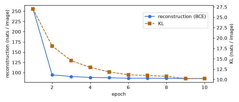
epoch  1 | -ELBO  282.76 = 재구성  255.74 + KL 27.03
epoch  2 | -ELBO  112.65 = 재구성   94.57 + KL 18.08
epoch  3 | -ELBO  105.07 = 재구성   90.51 + KL 14.56
…
epoch  9 | -ELBO   95.57 = 재구성   85.34 + KL 10.23
epoch 10 | -ELBO   95.95 = 재구성   85.72 + KL 10.23
VAE 학습 97.1초
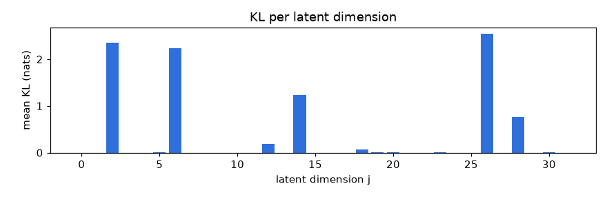
차원별 평균 KL (큰 순서 5개): z[26]=2.55, z[2]=2.35, z[6]=2.23, z[14]=1.23, z[28]=0.76
KL > 0.05 인 '살아 있는' 차원: 7개 / 32개
재구성 항(BCE)의 이론적 바닥값: 그림당 79.9 nats
그림 저장: figures
On a laptop GPU, 10 epochs of VAE training take about 30 seconds on their own; the run above, which shared the GPU with other training jobs, took about 97 seconds, and the full run including the comparison autoencoder took 2–4 minutes. With CPU only (4 threads), each step takes about 0.5 seconds, and the VAE and autoencoder together take about 50 minutes. Reducing to --epochs 3 gives nearly identical figures.
Reading the results
Learning curves and reconstruction
- The KL rises to 27 nats in the first epoch, then drops to around 10. At first the model uses the latent space generously to get reconstruction right, then finds ways to achieve the same reconstruction with less information.
- The reconstruction term is about 85 nats, close to the floor of about 80 nats. The remaining roughly 6 nats is what the model actually gets wrong.
- The KL term can be seen as an upper bound on the amount of information an image stores in \(z\). 10 nats is \(10/\ln 2 \approx 14.4\) bits, enough information to distinguish the angle in \(2^{14} \approx 16{,}000\) steps. In other words, the 4096 pixels actually held only a little over 14 bits of information.
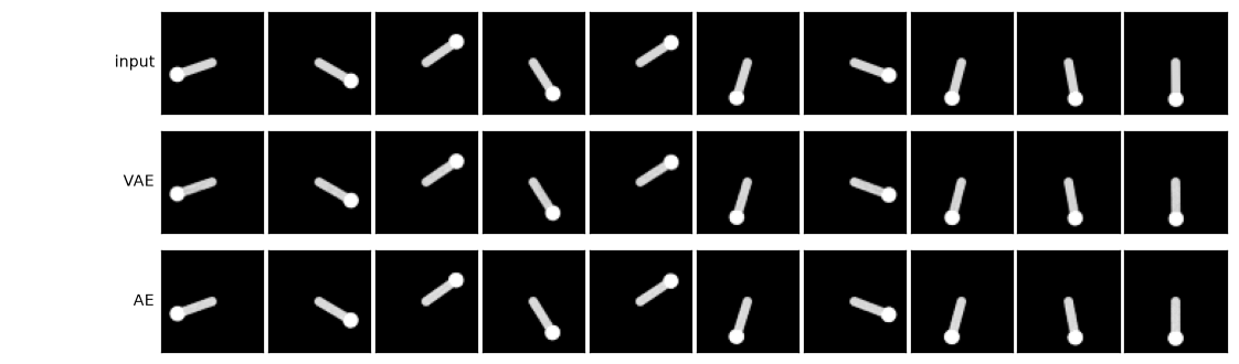
- In the reconstruction comparison (input, the VAE's reconstruction from the mean \(\mu\), and an autoencoder with the same architecture), both restore the angle accurately.
- Figure: Reconstruction and KL terms over epochs
- Figure: 10 inputs and their VAE and autoencoder reconstructions
Number of dimensions used
A per-dimension KL of 0 means that for that dimension, every image's \(q_\phi(z_j \mid x)\) equals \(\mathcal{N}(0, 1)\), so the dimension carries no information about the image. Because of the KL penalty, a VAE uses only the dimensions it needs and switches off the rest. Only 7 of the 32 were used (6–8 depending on the run).
There are two reasons why more than one dimension is used even though the only degree of freedom is the angle. The angle lives on a circle, returning to where it started after a full turn, so representing it without discontinuity requires at least 2 dimensions. Also, since the encoder and decoder are finite neural networks, they cannot lay the circle out as a clean circle and instead represent it as a bent loop spread over several dimensions. The representation a VAE finds is not a clean one but one that raises the ELBO.
Shape of the latent space
Projecting the latent vectors of 4,000 images onto 2 dimensions with principal component analysis (PCA) and coloring them by the true angle, both the VAE and the autoencoder give a closed loop whose color changes continuously with the angle. Without being told the angle, they found from images alone that the data lies on a circle. The difference is scale.
| VAE | Autoencoder | |
| Maximum absolute component value | About 3 | About 36 |
| Range along principal axes | Within ±3 (where \(\mathcal{N}(0, I)\) mostly lies) | Around ±60 |
The VAE's loop looks twisted because it is a 2-dimensional shadow of a loop in a space of about 7 dimensions.
Latent traversal
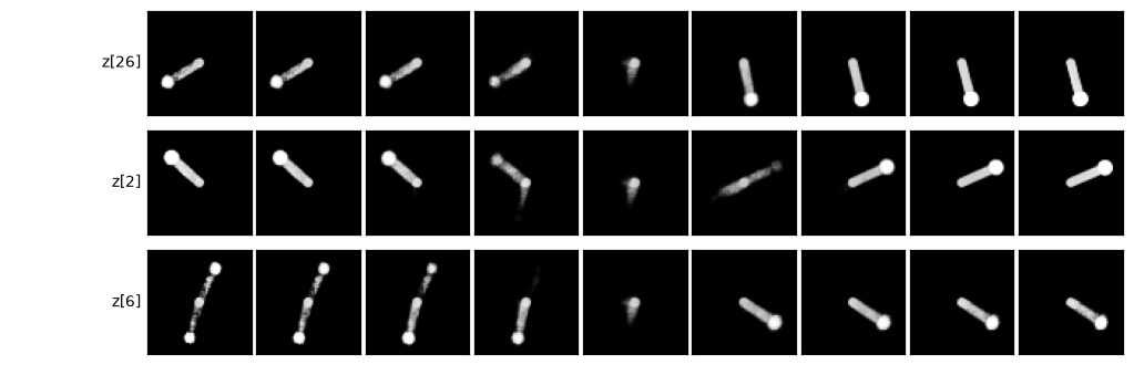
We take each of the three most informative dimensions in turn, keep the other dimensions at 0, vary only that dimension from −3 to 3 in 9 steps, and decode (latent traversal). Moving one dimension rotates the rod, but no single dimension maps cleanly to the angle. Partway through, the rod becomes blurry or two angles appear overlaid. Because the loop-shaped data is spread across several axes, moving along one axis alone passes through regions off the loop. Having each dimension handle only one human-interpretable property is called disentanglement, and an ordinary VAE does not guarantee it.
Sampling from the prior
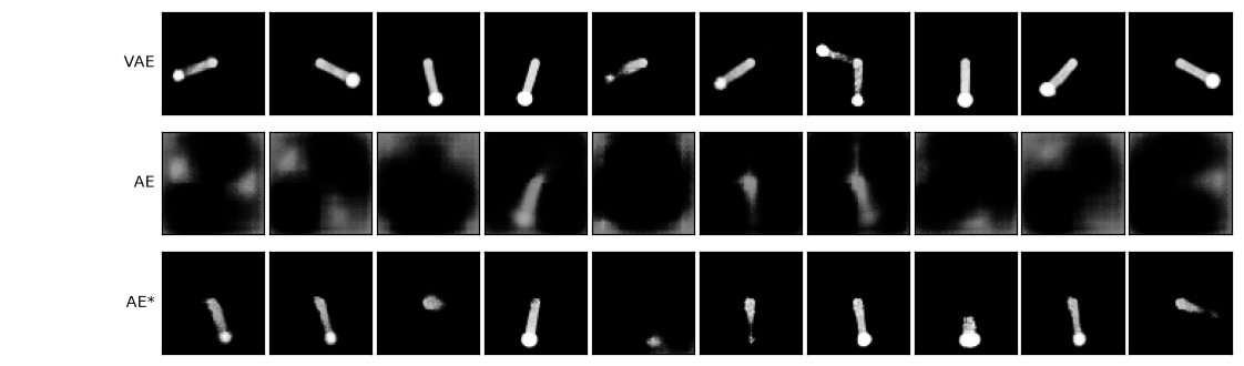
When we sample \(z \sim \mathcal{N}(0, I)\) and decode, the VAE produces a pendulum image for almost every \(z\) (occasionally a blurry image or one with two overlapping rods). The autoencoder receives a \(z\) at the wrong scale and produces meaningless smudges, and even when sampling each dimension to match its actual mean and standard deviation (AE*), many images still look wrong. The autoencoder's data lies only on a thin loop in a large space, and points sampled independently per dimension mostly fall off that loop. Since the M model in chapter 9 keeps sampling new \(z\) in latent space to imagine the future, this difference separates eyes that can be used for imagination from eyes that cannot.
β-VAE and the KL weight
Adding a weight \(\beta\) to the KL term of the loss gives the β-VAE (Higgins et al., 2017).
\(\mathcal{L}_\beta = \mathbb{E}_{q_\phi}\big[-\log p_\theta(x \mid z)\big] + \beta\,D_{\mathrm{KL}}\big(q_\phi(z \mid x)\,\Vert\,p(z)\big)\)
- \(\beta \gt 1\): pushes the model to use less information. The latent space tends to be smoother and more disentangled (not guaranteed), but reconstructions get blurrier.
- \(\beta \lt 1\): reconstructions get sharper, but the latent space becomes sparse like an autoencoder's. With \(\beta = 0\) it is nearly the same as an autoencoder (with \(\sigma\)).
\(\beta\) plays the same role as the variance \(s^2\) of a Gaussian decoder. Plugging the Gaussian decoder's negative log-likelihood into −ELBO and multiplying both sides by the positive number \(2s^2\) (which does not move the minimum) gives the same form as a β-VAE with squared error.
\(\begin{align} -\text{ELBO} &= \frac{1}{2s^2}\,\mathbb{E}_{q_\phi}\big\lVert x - \hat{x}\big\rVert^2 + D_{\mathrm{KL}} + \text{상수} \\ 2s^2 \cdot (-\text{ELBO}) &= \mathbb{E}_{q_\phi}\big\lVert x - \hat{x}\big\rVert^2 + 2s^2\,D_{\mathrm{KL}} + \text{상수}' \end{align}\)
\(\beta = 2s^2\)
The larger the pixel error the decoder assumes (the larger \(s\)), the less weight it gives to reconstruction and the more to KL. Merely switching MSE between a pixel mean and a pixel sum effectively changes \(\beta\) by a factor of 4096.
Posterior collapse and remedies
If the KL term or the decoder is too strong, the model can fall into a state where the encoder outputs \(q_\phi(z \mid x) = \mathcal{N}(0, I)\) for every image (KL = 0) and the decoder ignores \(z\), producing only an average image. This is posterior collapse. The 25 switched-off dimensions in this chapter are a partial, per-dimension collapse, and they switched off because their information was not needed, so they are not a problem. The problem is when every dimension switches off.
- Gradually increasing the KL weight (KL annealing)
- For the first few thousand steps, \(\beta\) is raised slowly from 0 to 1 so the model learns reconstruction first.
- Free bits, KL tolerance
- No penalty is applied when the KL is below a set value \(c\). The loss uses \(\max(D_{\mathrm{KL}}, c)\). In the region \(D_{\mathrm{KL}} \lt c\), the gradient of this term is 0, so the pressure to squeeze the KL down to 0 disappears. It is the same technique as free nats in chapter 11. Ha & Schmidhuber's public code applies a tolerance of 0.5 nats per dimension, 16 nats in total over 32 dimensions, to the summed KL (
kl_tolerance; this does not appear in the paper itself), and DreamerV3 in chapter 12 uses 1 nat of free bits. - Monitoring per-dimension KL
- Plotting a bar chart of per-dimension KL during training shows right away whether the number of informative dimensions is collapsing to 0.
What chapter 9 needs
When the code finishes running, it leaves two files, which chapters 9 and 10 start from.
| File | Contents | Used in |
| | The trained VAE (loaded with | Chapter 9: converting episodes into \(z\) sequences, rendering dream images. Chapter 10: converting real environment images into \(z\) |
| | Images, actions, rewards, and ground-truth states (for checking) from 200 episodes | Chapter 9: MDN-RNN training data |
We can now summarize an image as 32 numbers, but a single image cannot tell how fast the pendulum is spinning. Chapter 9 builds a memory (MDN-RNN) that remembers past frames and predicts the next \(z\).
Summary
- Images (4096 dimensions) actually lie in a much lower dimension. A World Model compresses images into a small latent vector \(z\) and predicts the future in that space.
- An autoencoder reconstructs well, but since we don't know where its latent space lies or what shape it has, we cannot sample new \(z\) from it.
- A VAE assumes the generative process \(z \sim \mathcal{N}(0, I),\ x \sim p_\theta(x \mid z)\) and maximizes the ELBO in place of the intractable \(\log p_\theta(x)\).
- \(\log p_\theta(x) = \text{ELBO} + D_{\mathrm{KL}}(q_\phi(z\mid x)\,\Vert\,p_\theta(z\mid x))\), and ELBO = reconstruction term − \(D_{\mathrm{KL}}(q_\phi(z\mid x)\,\Vert\,\mathcal{N}(0,I))\).
- The closed form of the KL term is \(\tfrac{1}{2}\sum_j(\mu_j^2 + \sigma_j^2 - 1 - \log\sigma_j^2)\). A Bernoulli decoder gives BCE, and a fixed-variance Gaussian decoder gives MSE.
- Reparameterization, \(z = \mu + \sigma\odot\epsilon\), lets gradients flow even through random sampling.
- The pendulum VAE discovered the angle as a closed loop, used only about 7 of its 32 dimensions, and produces plausible images from \(z\) sampled from \(\mathcal{N}(0, I)\).
Exercises
- 1. Computing KL
- For \(q = \mathcal{N}(1, 0.25)\) (\(\mu = 1\), \(\sigma = 0.5\)), \(D_{\mathrm{KL}}(q\,\Vert\,\mathcal{N}(0,1))\) is \(\tfrac{1}{2}(1 + 0.25 - 1 + 1.386) = \tfrac{1}{2}(1.636) \approx 0.818\) nats.
- 2. ELBO and the gap
- If \(\log p_\theta(x) = -90\) and the ELBO is \(-95\), then \(D_{\mathrm{KL}}(q_\phi(z\mid x)\,\Vert\,p_\theta(z\mid x)) = -90 - (-95) = 5\). If training only the encoder raises the ELBO to \(-92\), \(\log p_\theta(x)\) stays the same, so the KL drops from \(5 \to 2\).
- 3. Reparameterization
- For \(f(z) = 3z + 1\), \(\mathbb{E}[f(z)] = 3\mu + 1\), so \(\partial/\partial\mu = 3\) and \(\partial/\partial\sigma = 0\). The formula agrees: from \(f'(z) = 3\), \(\mathbb{E}[3] = 3\) and \(\mathbb{E}[3\epsilon] = 0\). The expectation of a linear function does not depend on the variance.
- 4. Output sizes
- With a 96×96 input, the encoder gives \(96 \to 47 \to 22 \to 10 \to 4\), and the flattened length is 256 × 4 × 4 = 4096. The input size of
fc_muandfc_logvarmust change from 1024 to 4096. Left unchanged, the decoder still outputs 64×64, so the transposed convolutions must also be modified to reconstruct 96×96. - 5. The loss scale trap
- If the reconstruction loss is changed from a pixel sum to a pixel mean (with KL unchanged), multiplying the whole loss by 4096 shows it equals "reconstruction (sum) + 4096 × KL". This makes it a β-VAE with \(\beta = 4096\), so most dimensions switch off and images become very blurry. Changing only
reduction="mean"invae_lossalso divides by the batch size once more, so the trailing/ batchmust be removed as well to match this calculation. - 6. Trying different β
- Compare per-dimension KL and prior samples with
python ch08_vae.py --beta 4and--beta 0.25. The original tutorial expects that a larger \(\beta\) reduces the number of active dimensions and blurs the samples, while a smaller one increases the dimensions and produces more odd samples.
See also
- World Models:Tutorial
- World Models
- VAE
- Autoencoder
- Recurrent World Models Facilitate Policy Evolution
- Maximum likelihood estimation
- Bayes' theorem
- Cross entropy
- Normal distribution
- Convolution arithmetic