WorldModels:Tutorial:07-PlanningMPC
lastmod 2026-11-18created 2026-11-172 edits
Planning in Imagination: MPC and CEM is chapter 7 of the World Model tutorial. Using the dynamics model trained in chapter 6, it tries out hundreds of action sequences in imagination, executes only the first action of the best one, and then replans. This model predictive control (MPC) is used to swing up and balance a pendulum. It uses only a model and search (random shooting, CEM), with no policy network and no reward learning. The second half covers probabilistic ensembles and PETS, which let the model reveal where it does not know.
- Original: 07. Planning in Imagination: MPC and CEM
- Code:
code/ch07_mpc.py(about 6–10 minutes on 4 threads of a laptop CPU, a little over 20 seconds with--quick) andcode/ch07_pets.py(about 20 minutes, around 1 minute with--quick).ch06_dynamics.pyandwm_envs.pymust be in the same folder. - Previous: 06. The First World Model / Next: 08. VAE
Planning: optimizing an action sequence
Given the current observation \(o_t\), once an action sequence \(a_{t:t+H-1} = (a_t, a_{t+1}, \dots, a_{t+H-1})\) for the next \(H\) steps is chosen, the World Model \(f_\theta\) can imagine its outcome without executing it.
\(\hat o_t = o_t, \qquad \hat o_{t+k+1} = f_\theta(\hat o_{t+k},\ a_{t+k}) \quad (k = 0, 1, \dots, H-1)\)
The sum of rewards along the imagined trajectory is the score of that action sequence.
\(J(a_{t:t+H-1}) = \sum_{k=0}^{H-1} r\big(\hat o_{t+k},\ a_{t+k}\big)\)
Planning is the optimization problem of finding the action sequence that maximizes this score.
\(a^*_{t:t+H-1} = \operatorname*{arg\,max}_{a_{t:t+H-1}\ \in\ [-2,\,2]^H}\ J(a_{t:t+H-1})\)
- \([-2, 2]^H\) is the set of all length-\(H\) vectors whose components lie between \(-2\) and \(2\) (the pendulum's torque range).
- The reward \(r\) is the known function
pendulum_reward. The model only stands in for the next observation. - The reinforcement learning of chapter 5 trains a policy \(\pi(a \mid s)\) in advance and evaluates it once when acting. Planning learns no policy; it computes each action on the spot by optimization. This is computationally heavy, but when the reward function changes, the agent can plan for the new goal without retraining.
Why exhaustive search is not feasible
Even if actions are discretized into just five values \(\{-2, -1, 0, 1, 2\}\), there are \(5^{25} \approx 3\times10^{17}\) action sequences for \(H = 25\). Testing a million per second would take over 9,000 years. A method that tests only a subset is therefore needed, and this chapter uses two derivative-free, sample-based methods (random shooting and CEM). They are simple to implement, well suited to evaluating hundreds of candidates at once as a batch, and work even when the model is not smooth (e.g., clipped angular velocity). Methods that differentiate through the model and adjust actions with gradients are covered in chapter 12.
Scoring candidate action sequences
Both methods use a function that scores \(N\) candidate action sequences at once.
@torch.no_grad()
def evaluate_sequences(model, obs, actions):
    """후보 행동열 N 개를 모델 속에서 굴려, 각 행동열의 예측 총 보상 J 를 계산한다.

    obs     : (3,)        지금의 진짜 관측 o_t (여기서 상상을 시작한다)
    actions : (N, H, 1)   후보 행동열 N 개, 각각 길이 H
    반환    : (N,)        J = Σ_k r(ô_{t+k}, a_{t+k})
    """
    N, H, _ = actions.shape
    o = obs.expand(N, -1)  # (N, 3): 모든 후보가 같은 곳에서 출발
    total = torch.zeros(N, device=actions.device)
    for k in range(H):
        a = actions[:, k]  # (N, 1)
        total += pendulum_reward(o, a)  # 알려진 보상 함수로 점수를 매긴다
        o, _ = model.predict(o, a)  # 상상 속 다음 관측
    return total
-
obs.expand(N, -1)makes a single observation look as if it were copied \(N\) times, without copying memory. - The loop runs only over time \(k\). Candidates are the batch dimension, so even with \(N = 400\) the network is called only \(H\) times.
Model predictive control (MPC)
The \(H\)-step action sequence obtained by planning is not executed to the end, because, as seen in chapter 6, imagination becomes less accurate the longer it runs. Instead, the following is repeated at every step.
- Plan \(H\) steps from the current real observation \(o_t\): \(a^*_{t:t+H-1}\).
- Execute only the first action \(a^*_t\) in the real environment.
- Receive the new real observation \(o_{t+1}\), return to step 1, and replan from scratch.
This is model predictive control (MPC). Because the planning window slides forward one step at a time, it is also called receding horizon control. It came into wide use in chemical process control in the 1970s and 1980s and is now a basic tool for controlling robots and autonomous vehicles. At every step it builds an \(H\)-step plan, but only the first step is executed; the rest is imagined and then discarded (Figure 7-1 in the original). It is like driving at night: you look at the 50 m lit by the headlights, turn the wheel slightly, and a second later decide again based on the newly visible 50 m.
MPC suits the error accumulation problem of chapter 6 for two reasons.
- Short imagination: only \(H\) steps are imagined, so the rollout stops before errors pile up without bound.
- Feedback: every step restarts from the real observation (closed loop), so the errors of the previous plan do not carry over into the next one.
The price is computation: choosing a single action calls the model tens of thousands of times. With large models this becomes heavy, which is why methods such as Dreamer in chapter 12 learn a policy in imagination instead of planning.
In the code, run_episode(env, planner) (region run_episode in ch07_mpc.py) calls planner(obs) again with the new observation at every step. The planner returns only the first action to execute, not the whole plan.
Random shooting
The simplest planner:
- Draw \(N\) random action sequences uniformly from \([-2, 2]\).
- Compute the score \(J\) of each one inside the model.
- Pick the first action of the highest-scoring sequence.
RandomShootingPlanner (region random_shooting, default horizon=25, n_candidates=1000) implements this procedure. Early work combining neural-network World Models with MPC (Nagabandi et al., 2018) also used random shooting. However, it hits a limit as the horizon grows.
Probability of drawing a good candidate
Suppose a fraction \(p\) of random action sequences are good enough, and \(N\) are drawn independently.
\(\begin{align} P(\text{none is good}) &= (1-p)^N = e^{N\log(1-p)} \\ P(\text{at least one is good}) &= 1 - (1-p)^N \approx 1 - e^{-pN} \end{align}\)
The approximation uses \(\log(1-p) \approx -p\) for small \(p\) (\(\log(1+x)\) has value 0 and slope 1 at \(x=0\)). \(pN\) is the expected number of good candidates: at around 1 the chance of getting a good candidate is about 63%, and at 3 it is about 95%.
- Example: with \(p = 0.001\) and \(N = 1000\), the exact value is \(1 - 0.999^{1000} = 0.6323\) and the approximation is \(1 - e^{-1} = 0.6321\).
- The problem is that \(p\) shrinks exponentially with the horizon \(H\). Even if half of the actions are acceptable at each step, the fraction that is acceptable at all 25 steps is \(0.5^{25} \approx 3\times10^{-8}\). A method that samples more densely near good candidates is needed.
Cross-entropy method (CEM)
The cross-entropy method (CEM) repeats random shooting several times, each time resampling near the candidates that did well in the previous round (Rubinstein, 1999). It places one Gaussian on each component of the action sequence.
\(a_{t+k} \sim \mathcal{N}(\mu_k,\ \sigma_k^2), \qquad k = 0, 1, \dots, H-1\)
One iteration is as follows.
- Sample: draw \(N\) action sequences, \(a^{(i)}_{t+k} = \mu_k + \sigma_k\,\epsilon^{(i)}_k\) with \(\epsilon \sim \mathcal{N}(0, 1)\), and clip them to \([-2, 2]\).
- Score: compute \(J\) for each candidate inside the model.
- Select elites: take the top \(K\) candidates by score as the elites.
- Refit: replace \(\mu\) and \(\sigma\) with the Gaussian that best fits the \(K\) elites.
Repeating this a few times (5 here) moves the Gaussian toward good action sequences and narrows it. The final mean \(\mu_0\) is the first action to execute.
In the original's 2D demo (60 samples, 10 elites, a score function with one high peak and one low peak), the ellipse (mean ± 2σ) narrows onto a peak after five or six iterations, but roughly one run in ten gets stuck on the low peak. CEM is a local search that does not guarantee the global optimum.
Refitting to the elites is maximum likelihood estimation
Step 4 is the maximum likelihood estimation of chapter 2. Looking at a single component, it maximizes the log-likelihood of the elite values \(x_1, \dots, x_K\).
\(\begin{align} \ell(\mu, \sigma^2) &= \sum_{i=1}^K \log\mathcal{N}(x_i;\mu,\sigma^2) = \sum_{i=1}^K\left[-\frac12\log(2\pi\sigma^2) - \frac{(x_i - \mu)^2}{2\sigma^2}\right] \\ &= -\frac{K}{2}\log(2\pi) - \frac{K}{2}\log\sigma^2 - \frac{1}{2\sigma^2}\sum_{i=1}^K (x_i-\mu)^2 \end{align}\)
Differentiating with respect to \(\mu\) and setting it to 0 gives the mean.
\(\frac{\partial \ell}{\partial \mu} = \frac{1}{\sigma^2}\sum_{i=1}^K (x_i - \mu) = 0 \ \Rightarrow\ \hat\mu = \frac1K\sum_{i=1}^K x_i\)
Treating \(v = \sigma^2\) as a single variable, differentiating and setting it to 0 gives the variance.
\(\frac{\partial \ell}{\partial \sigma^2} = -\frac{K}{2\sigma^2} + \frac{1}{2(\sigma^2)^2}\sum_{i=1}^K (x_i-\mu)^2 = 0 \ \Rightarrow\ \hat\sigma^2 = \frac1K\sum_{i=1}^K (x_i - \hat\mu)^2\)
The sample mean and sample variance of the elites (dividing by \(K\), i.e., the biased sample variance) are the new Gaussian. elites.mean(dim=0) and elites.std(dim=0, unbiased=False) in the code are these two formulas.
This is also where the name "cross-entropy" comes from. The cross entropy (chapter 3; here \(H(\cdot,\cdot)\) is not the planning horizon) between the distribution \(\hat p\) that assigns probability \(\frac1K\) to each elite and the Gaussian \(q\) is
\(H(\hat p, q) = -\mathbb{E}_{x\sim\hat p}[\log q(x)] = -\frac1K\sum_{i=1}^K \log q(x_i)\)
so minimizing the cross entropy is the same as maximizing the log-likelihood of the elites. It finds the Gaussian that best imitates the distribution of the elites.
Smoothing and warm start
Smoothing: instead of switching to the new values at once, mix in a fraction \(\alpha\) of the old values.
\(\mu \leftarrow \alpha\,\mu_{\text{old}} + (1-\alpha)\,\hat\mu, \qquad \sigma \leftarrow \alpha\,\sigma_{\text{old}} + (1-\alpha)\,\hat\sigma\)
- With \(\alpha = 0.1\), the new values get 90% of the weight. Example: with \(\mu_{\text{old}} = 0\) and \(\hat\mu = 1.5\), \(\mu = 1.35\).
- It prevents \(\sigma\) from suddenly collapsing toward 0 when the elites happen to cluster on one side, which would stop further exploration.
- The public PETS implementation mixes the variance \(\sigma^2\) rather than the standard deviation with the same formula. Here \(\sigma\) is mixed; the effect is the same.
Warm start: the plan \(\mu_{0:H-1}\) from the previous step is a good starting point for the current step as well. Since its first action has already been executed, the plan shifted by one step, \((\mu_1, \mu_2, \dots, \mu_{H-1}, 0)\), is used as the initial mean of the current plan. This reaches a good plan in fewer iterations than starting from 0 every time.
class CEMPlanner:
    """교차 엔트로피 방법(CEM): 가우시안에서 행동열을 뽑고, 정예(elite)에 가우시안을 다시 맞추기를 되풀이한다."""

    def __init__(self, model, horizon=25, n_candidates=400, n_elites=40, n_iters=5,
                 alpha=0.1, init_std=1.0, device="cpu"):
        self.model, self.H, self.N, self.K = model, horizon, n_candidates, n_elites
        self.n_iters, self.alpha, self.init_std, self.device = n_iters, alpha, init_std, device
        self.reset()

    def reset(self):
        # 에피소드가 시작될 때 평균 행동열을 0 으로 (= 아무 정보 없음)
        self.mean = torch.zeros(self.H, 1, device=self.device)

    def evaluate(self, obs, actions):
        # 후보 행동열의 점수. 확률적 모델(ch07_pets.py)은 이 메서드만 바꿔 끼운다.
        return evaluate_sequences(self.model, obs, actions)

    def __call__(self, obs):
        obs = torch.as_tensor(obs, dtype=torch.float32, device=self.device)
        mean = self.mean.clone()  # (H, 1) μ
        std = torch.full_like(mean, self.init_std)  # (H, 1) σ
        for _ in range(self.n_iters):
            # 1) 표본 뽑기: a = μ + σ ⊙ ε,  ε ~ N(0, I). 범위 밖은 잘라낸다.
            eps = torch.randn(self.N, self.H, 1, device=self.device)
            actions = (mean + std * eps).clamp(-MAX_U, MAX_U)  # (N, H, 1)
            # 2) 모델 속에서 점수 매기기
            returns = self.evaluate(obs, actions)  # (N,)
            # 3) 점수 상위 K 개 = 정예
            elites = actions[returns.topk(self.K).indices]  # (K, H, 1)
            # 4) 정예에 가우시안을 최대우도로 맞춘다: 평균 = 표본 평균, 분산 = 표본 분산
            new_mean = elites.mean(dim=0)
            new_std = elites.std(dim=0, unbiased=False)
            # 5) 평활: 한 번에 너무 크게 바뀌지 않게 옛 값을 α 만큼 섞는다
            mean = self.alpha * mean + (1 - self.alpha) * new_mean
            std = self.alpha * std + (1 - self.alpha) * new_std
        # 웜 스타트: 다음 시각의 계획은 이번 계획을 한 칸 당긴 것에서 시작한다
        self.mean = torch.cat([mean[1:], torch.zeros(1, 1, device=self.device)])
        return mean[0].cpu().numpy()  # 첫 행동만 실행한다 (MPC)
Only the mean is carried over by the warm start; the standard deviation restarts from init_std at every step. The evaluate method is kept separate so that PETS can swap out just this part.
Hyperparameters
| Name | Value in this chapter | Increasing it | Decreasing it |
| Horizon \(H\) | 25 (1.25 s) | Considers the farther future, but model errors accumulate and computation grows | Becomes short-sighted and cannot find behaviors like "first swing the other way" |
| Number of candidates \(N\) | 400 | Higher chance of finding a better action sequence, more computation | Coarser search |
| Number of elites \(K\) | 40 (10%) | The Gaussian narrows slowly (more exploration) | Narrows quickly (risk of getting stuck in the wrong place) |
| Iterations | 5 | More precise optimization, more computation | Less precise |
| Smoothing \(\alpha\) | 0.1 | Slower changes | Fits the elites immediately |
| Initial \(\sigma\) | 1.0 | Explores widely at first | Looks only near the mean from the start |
With these settings, choosing one action calls the model \(5\times400\times25 = 50{,}000\) times (125 batched calls), and a single 200-step episode takes ten million calls. On 4 threads of a laptop CPU, one action took about 0.09 s and one episode about 18 s.
Balancing the pendulum: the model-based reinforcement learning loop
Since there is almost no data at first, the following loop is repeated (Figure 7-2 in the original).
- Data \(\mathcal{D}\): initially one episode of random actions.
- Train the model:
train_modelfrom chapter 6. - Run one episode (200 steps) in the real environment with CEM-MPC.
- Add the new experience (one episode = 200 transitions) to the data and return to step 2.
Acting by planning with the model collects data from places that random actions never reach (e.g., the upright position), and the model becomes accurate there too.
    # 1) 시드 데이터: 무작위 행동 에피소드 몇 개
    env = Pendulum(seed=args.seed)
    data = collect_episodes(env, args.seed_episodes, seed=args.seed)
    print(f"seed data: {args.seed_episodes} random episodes, "
          f"mean return {np.mean([ep['reward'].sum() for ep in data]):.1f}")

    # 2) 되풀이: 모델 학습 → 그 모델로 계획하며 진짜 환경에서 한 에피소드 → 데이터에 더하기
    returns_per_iter = []
    for it in range(1, args.iterations + 1):
        model, loss = fit_model(data, device, seed=args.seed + it, train_steps=train_steps)
        planner = CEMPlanner(model, horizon=args.horizon, device=device)
        episode, ret = run_episode(env, planner)
        data.append(episode)
        returns_per_iter.append(ret)
        print(f"iter {it:2d} | data {len(data):2d} episodes | model loss {loss:.5f} | "
              f"CEM-MPC return {ret:8.1f} | {time.time() - start:5.0f}s")
The model is retrained from scratch at every iteration. fit_model sets the number of epochs so that training takes about 3,000 gradient steps (batch size 256) regardless of data size. This is slower than continuing training, but it is simple and stable because weights fitted to old data do not interfere with learning from new data. The defaults are 1 seed episode and 8 iterations.
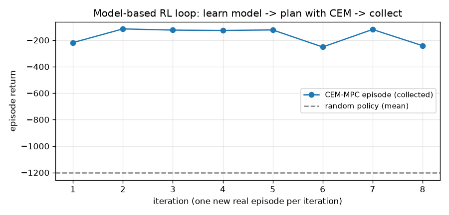
seed data: 1 random episodes, mean return -1071.9
iter  1 | data  2 episodes | model loss 0.00005 | CEM-MPC return   -218.4 |    40s
iter  2 | data  3 episodes | model loss 0.00005 | CEM-MPC return   -114.7 |    70s
iter  3 | data  4 episodes | model loss 0.00007 | CEM-MPC return   -123.9 |   103s
iter  4 | data  5 episodes | model loss 0.00010 | CEM-MPC return   -126.4 |   128s
iter  5 | data  6 episodes | model loss 0.00005 | CEM-MPC return   -122.5 |   164s
iter  6 | data  7 episodes | model loss 0.00014 | CEM-MPC return   -251.5 |   209s
iter  7 | data  8 episodes | model loss 0.00010 | CEM-MPC return   -119.0 |   244s
iter  8 | data  9 episodes | model loss 0.00007 | CEM-MPC return   -241.5 |   291s
- With a model trained on a single random episode (200 transitions), the first MPC episode already scored \(-218\). The pendulum has only a 3-dimensional state and smooth physics, so 200 transitions are enough for a model accurate enough to swing up.
- The return swinging between \(-115\) and \(-250\) across iterations is mainly due to the starting state. Episodes that start near the bottom and need an extra swing land near \(-250\); episodes that get up in one swing land near \(-115\).
- Figure: CEM-MPC episode return per iteration and the random policy average
Comparing the three methods
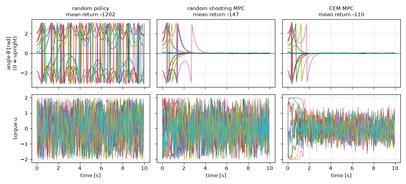
Results of comparing the three methods from the same 10 starting states, using one model trained on the final data (9 episodes):
random policy       : mean return  -1202.1 ±  183.2  (episodes: -866, -1248, -1183, -1173, -1397, -1307, -1506, -1296, -1068, -975)
random shooting MPC : mean return   -147.1 ±  106.4  (episodes: -1, -119, -125, -120, -243, -123, -366, -248, -126, -1)
CEM MPC             : mean return   -110.4 ±   66.6  (episodes: -0, -119, -126, -119, -124, -116, -249, -123, -128, -0)
| Method | Mean return (10 episodes) | Standard deviation | Model calls per action |
| Random policy | \(-1202.1\) | 183.2 | 0 |
| Random shooting MPC (\(N=1000\), \(H=25\)) | \(-147.1\) | 106.4 | 25,000 |
| CEM MPC (\(N=400\), \(K=40\), 5 iterations, \(H=25\)) | \(-110.4\) | 66.6 | 50,000 |
- CEM brings the pendulum upright within 3 seconds, and random shooting within about 4 seconds at the latest; both then hold it there until the end. With the random policy the angle keeps rotating.
- Random shooting's torque jumps between \(\pm2\) at every step even while balancing. CEM uses \(\pm2\) only during the swing-up and mostly stays within \(\pm1\) while balancing (some jitter remains), because it concentrates on refining the region around good action sequences.
- Episodes with a return close to 0 are those that started almost upright.
- The chapter 5 baselines (100 starting states) were about \(-1234\) for the random policy and about \(-183\) for a hand-crafted policy that uses the energy equation. CEM MPC's \(-110\) beats that without using any laws of physics. However, only 10 starting states are used here and the seeds differ, so this is not a rigorous comparison.
- Figure: Angle and torque trajectories for the three methods, 10 each
Key point: without any policy learning, the pendulum swing-up was solved with just "a World Model learned from data + search inside it (CEM) + replanning at every step (MPC)". Interaction with the real environment was only 9 episodes (1,800 steps). Doing trial and error inside the model instead of the real world is the most direct benefit of a World Model.
The model exploitation problem
The planner takes the model's scores at face value and searches for the action sequence that maximizes them. If the model wrongly predicts somewhere that "going here gives a huge reward", the planner will find that wrong spot. Optimization does not experience errors evenly; it seeks out and uses errors that happen to be wrong in its favor. This is model exploitation. It is like a student who finds a loophole in the grading criteria and gets a high score.
The most dangerous places are those without data. Predictions there are unconstrained, so if the planner happens to find an optimistic prediction, the actual outcome is nothing like what was expected. For the pendulum this was not a big problem because the model is smooth and the data is evenly spread, but it happens often in problems with many states and actions. There are three remedies.
- Keep running the loop: when an exploiting action is actually executed, its outcome enters the data and the model gets corrected.
- Shorten the horizon and replan often: keep wrong imagination from running on for long (MPC).
- Make the model aware of what it does not know: if the model can flag where it is unsure, optimistic predictions there need not be trusted. This is the topic of the second half of this chapter.
Probabilistic models: predicting the mean and variance together
The chapter 6 model predicted the next state as a single number. Now, for each output, it produces both a mean \(\mu_\theta(x)\) and a variance \(\sigma^2_\theta(x)\), predicting the next state as a distribution.
\(p_\theta(y \mid x) = \mathcal{N}\big(y;\ \mu_\theta(x),\ \sigma_\theta^2(x)\big)\)
The variance can differ for each input \(x\) (heteroscedastic). This lets the model distinguish states whose outcome is almost always the same from states whose outcome varies widely.
Gaussian NLL that also learns the variance
In chapter 6 the variance was fixed, so the NLL reduced to MSE. This time the model also sets the variance, so every term of the NLL stays. The network outputs the log variance \(s = \log\sigma^2\) instead of the variance. \(\sigma^2 = e^{s}\) is positive for any real \(s\), and very small and very large variances can be handled as numbers of similar magnitude.
\(\begin{align} -\log\mathcal{N}(y;\mu,\sigma^2) &= \frac12\log(2\pi) + \frac12\log\sigma^2 + \frac{(y-\mu)^2}{2\sigma^2} \\ &= \frac12\log(2\pi) + \frac12\left[(y-\mu)^2 e^{-s} + s\right] \end{align}\)
Dropping the constant \(\frac12\log 2\pi\) and multiplying by 2 does not move the minimum, so the loss is as follows. ((target - mean) ** 2) * torch.exp(-logvar) + logvar in the code is this formula.
\(\mathcal{L}(\mu, s) = (y - \mu)^2 e^{-s} + s\)
The two terms pull against each other. The gradients are:
\(\frac{\partial\mathcal{L}}{\partial\mu} = -\frac{2(y-\mu)}{\sigma^2}, \qquad \frac{\partial\mathcal{L}}{\partial s} = 1 - \frac{(y-\mu)^2}{\sigma^2}\)
- The gradient for the mean is the MSE gradient \(-2(y-\mu)\) divided by \(\sigma^2\). Errors where the model says the data is noisy (large variance) count less, and errors where it claims certainty count more.
- \(\frac{\partial\mathcal{L}}{\partial s} = 0 \Leftrightarrow \sigma^2 = (y-\mu)^2\). If the variance is smaller than the actual squared error, the gradient is negative and \(s\) increases; if larger, \(s\) decreases. Averaged over many data points, the learned variance matches the mean squared error near that input. The model learns to predict the size of its own error.
- Numerical example: with \(y = 1.0\), \(\mu = 0.4\), \(s = 0\), we get \(\mathcal{L} = 0.36\), \(\frac{\partial\mathcal{L}}{\partial\mu} = -1.2\) (increase \(\mu\)), and \(\frac{\partial\mathcal{L}}{\partial s} = 0.64\) (decrease \(s\); a variance of 1 is too large compared with the actual error of 0.36).
Caution: if \(\mu\) exactly matches the target at some data point, \(\mathcal{L} = s\), and \(s \to -\infty\) (variance → 0) can decrease without bound. Conversely, it is also possible to make \(s\) very large and wipe out the error term. That is why the log variance is confined to a range.
Bounding the log variance with softplus
Clipping with torch.clamp makes the gradient 0 outside the range, which stops learning. PETS bounds it smoothly with \(\mathrm{softplus}(x) = \log(1 + e^{x})\). Softplus is always greater than 0; it is a smooth ReLU that is \(\approx x\) for large \(x\) and \(\approx 0\) for very small \(x\).
\(\begin{align} s' &= s_{\max} - \mathrm{softplus}(s_{\max} - s_{\text{raw}}) \\ s &= s_{\min} + \mathrm{softplus}(s' - s_{\min}) \end{align}\)
- In the first formula \(s' \le s_{\max}\), and if \(s_{\text{raw}}\) is well below \(s_{\max}\), it passes through unchanged as \(s' \approx s_{\text{raw}}\). By the same logic, the second formula gives \(s \ge s_{\min}\).
- In the middle of the range \(s \approx s_{\text{raw}}\), and it bends smoothly at both ends. The gradient is nonzero everywhere. The exact upper limit is \(\log(e^{s_{\min}} + e^{s_{\max}})\), which exceeds \(s_{\max}\) by a negligible amount.
- Example: with \(s_{\max} = 0.5\) and \(s_{\text{raw}} = 3\), \(s' = 0.5 - \log(1 + e^{-2.5}) = 0.5 - 0.0789 = 0.421\). Then with \(s_{\min} = -10\), \(s = -10 + \log(1+e^{10.421}) \approx 0.421\).
- \(s_{\max}\) and \(s_{\min}\) are also learned parameters (initial values 0.5 and -10), and \(0.01\,(s_{\max} - s_{\min})\) is added to the loss so that the range does not grow needlessly wide.
Two kinds of uncertainty and ensembles
| Aleatoric uncertainty | Epistemic uncertainty | |
| Cause | The world itself is random (dice, sensor noise) | The model has not seen enough yet (lack of data) |
| With more data | Does not decrease | Decreases |
| Example | A ball thrown with the same force lands in slightly different places | The outcome of a state never visited before |
| In the model | The variance \(\sigma^2_\theta(x)\) output by each model | How much the predictions of several models disagree |
A single model that outputs a variance represents only aleatoric uncertainty. A single model cannot tell when it is confidently wrong where there is no data. So an ensemble of several trained models is used. The members give similar answers where there is data, and different answers where there is none, depending on their initialization and training path. The degree of disagreement is the epistemic uncertainty.
=== Total variance = aleatoric + epistemic === When \(E\) members each predict \(\mathcal{N}(\mu_e, \sigma_e^2)\), compute the variance of the mixture distribution obtained by picking a member uniformly at random and sampling from its distribution.
\(\begin{align} \mathbb{E}[y] &= \frac1E\sum_{e=1}^E \mu_e =: \bar\mu \\ \mathbb{E}[y^2] &= \frac1E\sum_{e=1}^E \mathbb{E}[y^2 \mid e] = \frac1E\sum_{e=1}^E (\sigma_e^2 + \mu_e^2) \\ \operatorname{Var}[y] &= \mathbb{E}[y^2] - \mathbb{E}[y]^2 = \frac1E\sum_e \sigma_e^2 + \frac1E\sum_e \mu_e^2 - \bar\mu^2 \\ &= \underbrace{\frac1E\sum_{e=1}^E \sigma_e^2}_{\text{aleatoric: mean of variances}} + \underbrace{\frac1E\sum_{e=1}^E (\mu_e - \bar\mu)^2}_{\text{epistemic: variance of means}} \end{align}\)
The first line uses the law of total expectation, and the second uses \(\operatorname{Var} = \mathbb{E}[y^2] - \mathbb{E}[y]^2\) within each member. The toy experiment toy_uncertainty_figure in the code computes the two terms separately: aleatoric = var.mean(0), epistemic = mu.var(0).
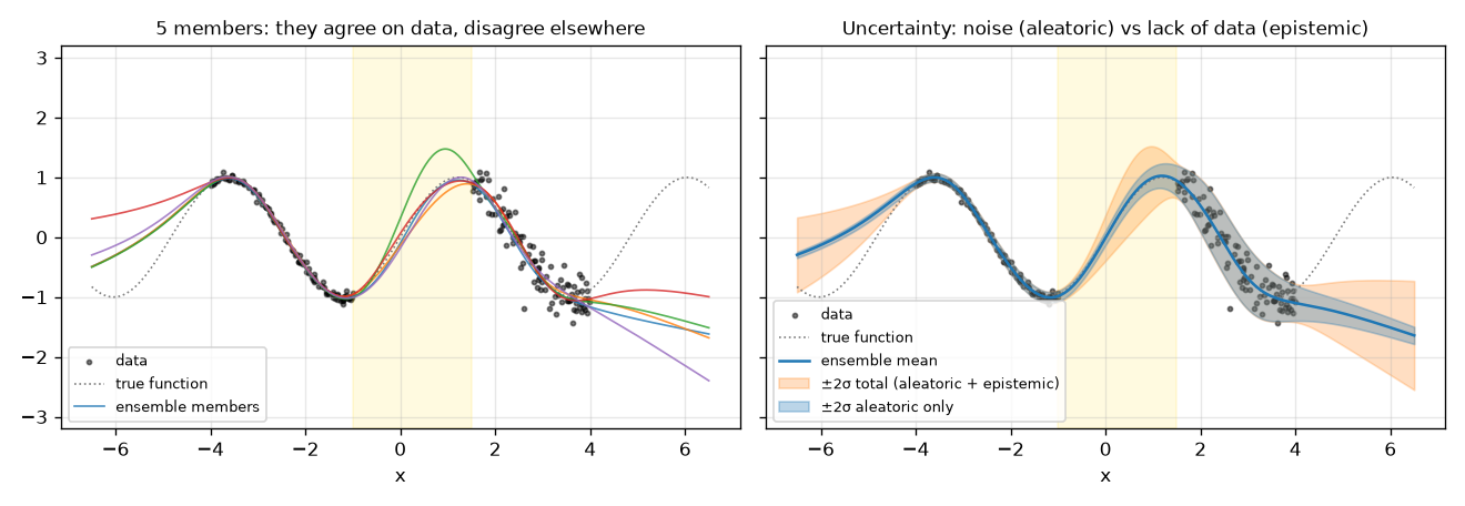
The toy problem is 1D regression \(y = \sin(1.3x) + \text{noise}\). Data exists only on \(x \in [-4,-1]\) (noise standard deviation 0.04, 100 points) and \([1.5, 4]\) (noise standard deviation 0.25, 100 points). There are 5 members with 64 hidden units.
  toy x=-2.50: aleatoric std 0.044, epistemic std 0.024
  toy x= 0.25: aleatoric std 0.071, epistemic std 0.238
  toy x= 2.75: aleatoric std 0.270, epistemic std 0.036
  toy x= 6.00: aleatoric std 0.080, epistemic std 0.389
- The learned aleatoric standard deviations (0.044, 0.270) recover the actual noise (0.04, 0.25) well.
- At \(x = 0.25\) and \(x = 6\), where there is no data, the epistemic standard deviations (0.238, 0.389) are nearly ten times larger than on the data (0.024, 0.036).
- The mean predictions of the five members overlap on the data and diverge in the gap and outside. However, at \(x \approx 6\) the true function lies outside the ±2σ band. Even an ensemble does not know everything outside the data.
- Figure: Per-member predictions for the 1D toy problem with aleatoric and total uncertainty bands
Bootstrap
To make the members disagree, each member gets not only a different initialization but also different training data. This is the bootstrap: drawing \(N\) samples with replacement from \(N\) data points. The probability that a given data point is never drawn is \(\left(1 - \frac1N\right)^N\), which approaches \(e^{-1} \approx 0.368\) for large \(N\) (the same calculation as the random shooting derivation with \(p = \frac1N\)). So each member sees only about 63.2% of the original data.
class EnsembleLinear(nn.Module):
    """E 개의 Linear 층을 배치 행렬곱 한 번으로 계산한다. x (E, B, in) → (E, B, out)."""

    def __init__(self, n_members: int, in_dim: int, out_dim: int):
        super().__init__()
        bound = 1.0 / math.sqrt(in_dim)  # nn.Linear 와 같은 초기화 범위
        self.weight = nn.Parameter(torch.empty(n_members, in_dim, out_dim).uniform_(-bound, bound))
        self.bias = nn.Parameter(torch.empty(n_members, 1, out_dim).uniform_(-bound, bound))

    def forward(self, x):
        return torch.baddbmm(self.bias, x, self.weight)  # bias + x @ weight  (멤버마다 따로)


class GaussianEnsemble(nn.Module):
    """멤버 E 개가 각자 평균 μ 와 로그 분산 log σ² 을 내는 확률적 앙상블."""

    def __init__(self, in_dim: int, out_dim: int, n_members: int = 5, hidden: int = 128):
        super().__init__()
        self.E = n_members
        self.layers = nn.ModuleList([
            EnsembleLinear(n_members, in_dim, hidden),
            EnsembleLinear(n_members, hidden, hidden),
            EnsembleLinear(n_members, hidden, hidden),
            EnsembleLinear(n_members, hidden, 2 * out_dim),  # 평균 + 로그 분산
        ])
        # 로그 분산의 위 · 아래 한계 (이것도 학습한다)
        self.max_logvar = nn.Parameter(torch.full((out_dim,), 0.5))
        self.min_logvar = nn.Parameter(torch.full((out_dim,), -10.0))

    def forward(self, x):
        h = x
        for layer in self.layers[:-1]:
            h = F.silu(layer(h))
        mean, raw_logvar = self.layers[-1](h).chunk(2, dim=-1)
        # softplus 로 부드럽게 [min_logvar, max_logvar] 안에 가둔다
        logvar = self.max_logvar - F.softplus(self.max_logvar - raw_logvar)
        logvar = self.min_logvar + F.softplus(logvar - self.min_logvar)
        return mean, logvar
-
EnsembleLinearkeeps the weights as a single tensor of shape(E, in, out)and computes all five members at once withtorch.baddbmm(batched matrix multiplication + bias). The input is also(E, B, in), so each member can receive a different input. - The last layer outputs twice the output dimension; the first half is used as the mean and the second half as the log variance before bounding.
def gaussian_nll(mean, logvar, target):
    """가우시안 음의 로그 가능도에서 상수(½ log 2π)와 앞의 ½ 을 뺀 것: (y − μ)²/σ² + log σ²."""
    return (((target - mean) ** 2) * torch.exp(-logvar) + logvar).mean()


def train_ensemble(model, X, Y, steps=3000, batch_size=256, lr=1e-3, device="cpu", seed=0):
    """X (N, in), Y (N, out) 는 numpy 배열 (진자에서는 호출하는 쪽이 미리 표준화한다). 멤버마다 부트스트랩 표본으로 학습한다.

    돌려주는 값은 마지막 미니배치의 손실(NLL + 로그 분산 범위 벌점)이다.
    """
    g = torch.Generator().manual_seed(seed)
    N, E = len(X), model.E
    X, Y = to_tensor(X, device), to_tensor(Y, device)
    boot = torch.randint(N, (E, N), generator=g).to(device)  # 멤버 e 의 데이터 = X[boot[e]] (복원 추출)
    opt = torch.optim.Adam(model.parameters(), lr=lr)
    for step in range(steps):
        pos = torch.randint(N, (E, batch_size), generator=g).to(device)
        idx = torch.gather(boot, 1, pos)  # (E, B): 멤버마다 자기 부트스트랩 목록에서 뽑은 번호
        mean, logvar = model(X[idx])  # (E, B, out)
        loss = gaussian_nll(mean, logvar, Y[idx])
        loss = loss + 0.01 * (model.max_logvar.sum() - model.min_logvar.sum())  # 한계를 좁게 유지
        opt.zero_grad()
        loss.backward()
        opt.step()
    return loss.item()
boot[e] is the list of bootstrap indices for member \(e\), and at every step each member draws a minibatch from its own list (torch.gather). The loss is the mean NLL over the five members plus \(0.01\sum_d (s_{\max,d} - s_{\min,d})\) (one term per output dimension).
PETS: planning with probabilistic ensembles
PETS (Probabilistic Ensembles with Trajectory Sampling, Chua et al., NeurIPS 2018) puts the pieces so far together. The model is a probabilistic ensemble, the planner is CEM, and what connects them is trajectory sampling (TS).
Trajectory sampling (TS∞)
With a probabilistic model, the outcome of an action sequence is not uniquely determined. So \(P\) particles are launched for each action sequence and rolled out separately.
- Each particle \(p\) is assigned one ensemble member \(e(p)\), which does not change until the end of the imagined rollout (hence TS∞).
- At every step a particle samples its next state from its member's distribution: \(\hat o^{(p)}_{k+1} = \hat o^{(p)}_k + \mu_{e(p)} + \sigma_{e(p)}\,\epsilon\), \(\epsilon \sim \mathcal{N}(0, I)\) (notation omits undoing the standardization).
- The score of an action sequence is the average of the particles' total rewards: \(\hat J = \frac1P\sum_{p=1}^P \sum_k r(\hat o^{(p)}_k, a_k)\).
Step 3 is a Monte Carlo estimate of the expected return \(\mathbb{E}[J]\). Step 1 is the key: fixing the member per particle means each particle lives in "one plausible world consistent with the data" until the end. Where the members disagree (where there is no data), the particles scatter into different worlds.
The PETS score is a simple average over particles, with no separate penalty term for uncertainty. Even so, model exploitation decreases for two reasons.
- Where only one member happens to be optimistically wrong, its score is pulled down when averaged with the particles of the other members.
- With a reward that penalizes the squared distance from the goal, the scatter itself lowers the average reward. Since \(\mathbb{E}[-\theta^2] = -\mathbb{E}[\theta]^2 - \operatorname{Var}[\theta]\), the loss equals the variance of the particles.
As a result, CEM tends to choose action sequences in regions where the models agree (where there is data).
The pendulum model ProbabilisticDynamics (region prob_dynamics) predicts the distribution of \([o_t, a_t] \to \Delta o_t\) with GaussianEnsemble(4, 3) and trains on standardized inputs and outputs. sample_next(obs, act) draws samples in the reparameterized form \(\mu + \sigma\odot\epsilon\) (chapter 8). The input shape is (E, B, 3), so the first dimension determines which member rolls it out.
@torch.no_grad()
def evaluate_sequences_ts(dyn, obs, actions, n_particles=10):
    """궤적 표본 전파(TS∞): 후보마다 입자 P 개를 띄우고, 입자마다 앙상블 멤버 하나를 끝까지 고정해 굴린다.

    obs (3,), actions (N, H, 1) → 기대 총 보상 (N,) = 그 후보에 속한 입자들의 총 보상 평균
    배치 모양: 멤버 E 개 × (후보 N × 멤버당 입자 m) — 후보 n 의 입자는 행 n·m … n·m+m−1.
    """
    N, H, _ = actions.shape
    E = dyn.E
    m = max(1, n_particles // E)  # 후보 하나에서 멤버 하나가 맡는 입자 수
    o = obs.expand(E, N * m, 3).clone()  # (E, N·m, 3) 모든 입자가 지금 관측에서 출발
    total = torch.zeros(E, N * m, device=actions.device)
    for k in range(H):
        a = actions[:, k].repeat_interleave(m, dim=0).expand(E, N * m, 1)  # 후보의 행동을 그 입자들에게
        total += pendulum_reward(o, a)
        o = dyn.sample_next(o, a)
    return total.view(E, N, m).mean(dim=(0, 2))  # 입자 평균 = 기대 리턴의 몬테카를로 추정


class PETSPlanner(CEMPlanner):
    """CEM 은 그대로 두고, 점수 매기기만 TS 입자 평균으로 바꾼 계획기."""

    def __init__(self, dyn, n_particles=10, **kwargs):
        super().__init__(dyn, **kwargs)
        self.P = n_particles

    def evaluate(self, obs, actions):
        return evaluate_sequences_ts(self.model, obs, actions, self.P)
- The batch is laid out with shape
(E, N·m, 3). For each of the \(N\) candidates, each member handles \(m = P/E\) particles, so each candidate gets \(P\) particles in total. -
repeat_interleave(m, dim=0)copies the actions of candidate \(n\) into rows \(nm, \dots, nm + m - 1\), and at the endview(E, N, m)reshapes back to take the per-candidate average. - With this chapter's settings (\(N = 200\), \(P = 10\), \(E = 5\), \(m = 2\)), each step computes \(5\times400 = 2{,}000\) rows.
Particles scatter where there is no data
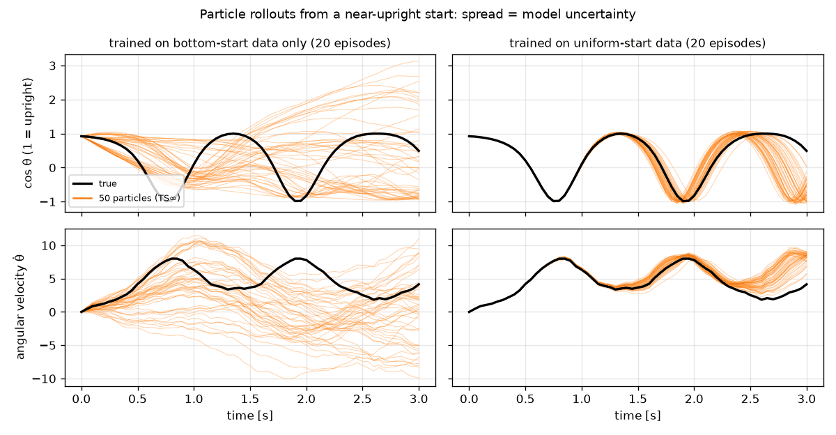
Two ensembles are trained and compared. One is trained only on 20 episodes that always start near the hanging position (random actions cannot reach the upper half, so the maximum of \(\cos\theta\) in this data is \(-0.33\)). The other is trained on 20 episodes with uniformly distributed starting positions. Both roll out 50 particles from an almost upright position (\(\theta = 0.4\)) with the same random action sequence (60 steps).
  bottom-start data only  : particle std of θ̇ at step 10/30/60 = 1.958 / 3.792 / 5.273
  uniform-start data      : particle std of θ̇ at step 10/30/60 = 0.037 / 0.455 / 0.753
- In the model that saw only bottom data, the particles scatter in all directions from the start, and it even imagines impossible values such as \(\cos\theta \gt 1\).
- In the model trained on uniform data, the particles stay tightly bunched along the true trajectory for a little over 2 seconds. The scatter of the particles becomes a signal that says "I don't know here".
- This signal has limits. Even with the uniform data, from about 2.3 seconds the particles spread a little, but the whole group drifts away from the truth, and the actual error is larger than the spread. When the members are wrong in the same direction, the ensemble does not notice.
- Figure: Rollouts of 50 particles starting from an almost upright position, with the true trajectory
Balancing the pendulum with PETS
The loop is the same as in the first half; only the model and planner change (region pets_loop). At every iteration a new ProbabilisticDynamics() is created and trained with fit(data, steps=3000), and one episode is run with PETSPlanner(dyn, n_particles=10, horizon=25, n_candidates=200, n_elites=30) and added to the data.
iter  1 | data  2 episodes | NLL  -8.821 | PETS return   -221.8 |   127s
iter  2 | data  3 episodes | NLL  -9.090 | PETS return   -115.1 |   261s
iter  3 | data  4 episodes | NLL  -7.906 | PETS return   -123.9 |   418s
iter  4 | data  5 episodes | NLL  -9.217 | PETS return   -127.0 |   532s
iter  5 | data  6 episodes | NLL  -8.947 | PETS return   -124.1 |   629s
iter  6 | data  7 episodes | NLL  -9.025 | PETS return   -253.8 |   682s
iter  7 | data  8 episodes | NLL  -9.100 | PETS return   -119.6 |   751s
iter  8 | data  9 episodes | NLL  -8.872 | PETS return   -243.3 |   796s
PETS (eval)         : mean return   -110.5 ±   66.4  (episodes: -1, -119, -123, -120, -125, -118, -248, -124, -128, -1)
- The mean return over 10 evaluation episodes is \(-110.5 \pm 66.4\), practically the same as the deterministic model + CEM (\(-110.4 \pm 66.6\)). The per-episode scores and the returns during the loop are also nearly identical.
- Computation is much heavier. On the same CPU, one action took about 0.23 s (200 candidates × 10 particles, 30 elites), 2.5 times the deterministic CEM (about 0.09 s, 400 candidates). The whole script took about 19 minutes while sharing the CPU with other workloads. On a GPU, one action took about 0.09 s, 2.6 times faster.
- The
NLLcolumn is the loss of the last training minibatch (mean NLL + range penalty). A value near \(-9\) means the log variance \(s\) went down close to the lower limit (initially \(-10\); it is learned and shifts slightly). The pendulum has no noise, so the model shrank the variance as far as it could. - Why the difference is small for the pendulum: there is no noise at all (zero aleatoric uncertainty) and the state is only 3-dimensional, so a few episodes of data cover almost everywhere. In the PETS paper, probabilistic ensembles clearly outperformed deterministic models on tasks with states of around twenty dimensions, such as robot arms and half-cheetah. Techniques for handling uncertainty pay off when the problem is hard and data is scarce, and computation grows by a factor of the particle count \(P\).
Pros and cons of planning with a World Model
| Pros | Cons |
| Can act right away without learning a policy | Heavy optimization for every action (tens of thousands of model calls) |
| When the reward function changes, plans for the new goal without retraining | Cannot consider anything beyond the horizon \(H\) (no value function) |
| Very little interaction with the real environment (data efficiency) | Sample-based search becomes hard as the action dimension and horizon grow |
| Replans at every step, correcting model errors through feedback | Model exploitation: the optimizer finds loopholes in the model |
- The inability to see beyond the horizon is addressed by adding a value function (an estimate of the reward obtainable from that point on) at the end of the horizon (TD-MPC in chapter 13).
- The heavy computation is addressed by learning a policy in imagination ahead of time (Dreamer in chapter 12).
Experiments suggested in the original:
- Shorten the horizon, e.g.,
python ch07_mpc.py --horizon 8, and see at what value it starts to fail (swinging up requires briefly moving the other way). - Set
n_itersofCEMPlannerto 1 and compare with random shooting. - Change
run_episodeto an open loop that executes the entire planned action sequence to the end. - Plan with a "stay still in the hanging position" reward instead of
pendulum_reward. The model does not need to be retrained.
Summary
- Planning is finding the action sequence that maximizes the total reward imagined in the model, \(J(a_{t:t+H-1}) = \sum_k r(\hat o_{t+k}, a_{t+k})\).
- MPC plans \(H\) steps at every step, executes only the first action, and then replans. Short imagination and feedback make it robust to model error.
- Random shooting is limited because the fraction \(p\) of good candidates shrinks exponentially with the horizon (\(1 - e^{-pN}\)).
- CEM repeatedly refits a Gaussian to the elites by maximum likelihood (mean = sample mean, variance = sample variance), and uses smoothing and warm start.
- The "collect → train → plan while collecting" loop balanced the pendulum after only 9 episodes of real experience (random \(-1202\) → CEM \(-110\)).
- A probabilistic model learns the mean and log variance together with the NLL \((y-\mu)^2e^{-s} + s\), and the learned variance matches the squared error.
- The total variance of an ensemble = mean of variances (aleatoric) + variance of means (epistemic). PETS feeds this uncertainty into planning with TS∞ particles.
Exercises
- 1. Number of candidates needed for random shooting
- With \(p = 10^{-4}\), how many candidates are needed for a 95% chance of getting at least one good candidate? From \(1 - e^{-pN} = 0.95\), \(pN = \log 20 \approx 3.0\), so \(N \approx 30{,}000\).
- 2. Running one CEM iteration by hand
- The \(K = 4\) elite values are \(1.0,\ 1.4,\ 1.8,\ 1.8\), with \(\mu_{\text{old}} = 0\), \(\sigma_{\text{old}} = 1\), \(\alpha = 0.1\). Since \(\hat\mu = 1.5\), \(\hat\sigma^2 = (0.25 + 0.01 + 0.09 + 0.09)/4 = 0.11\), and \(\hat\sigma = 0.3317\), we get \(\mu = 0.9\times1.5 = 1.35\) and \(\sigma = 0.1 + 0.9\times0.3317 = 0.3985\).
- 3. Equilibrium of variance learning
- For three data points with errors \(y - \mu = 0.1,\ -0.3,\ 0.2\) and a single log variance \(s\), which variance minimizes the total NLL? Differentiating with respect to \(s\) gives \(-e^{-s}\sum_i(y_i-\mu_i)^2 + 3 = 0\), so \(\sigma^2 = \frac{0.01+0.09+0.04}{3} = 0.0467\), which is the mean squared error.
- 4. Decomposing ensemble variance
- Three members predict \((\mu_e, \sigma_e^2) = (1.0, 0.04),\ (1.2, 0.04),\ (1.4, 0.07)\). Aleatoric = \(0.15/3 = 0.05\), \(\bar\mu = 1.2\), epistemic = \(0.08/3 \approx 0.0267\), total = \(0.0767\).
- 5. Why TS∞
- If the member is reselected at random at every step (TS1 in the PETS paper), a single particle effectively lives in a mix of worlds, so the systematic differences between members (epistemic uncertainty) are averaged at each step and partly cancel out. With TS∞, the differences between members keep growing until the end of the trajectory, so epistemic uncertainty shows up more clearly. The PETS paper tested both schemes, and the performance difference between them varied by task but was not large.
See also
- World Models:Tutorial
- World Models
- Reinforcement learning
- Policy
- Maximum likelihood estimation
- Cross entropy
- Normal distribution