WorldModels:Tutorial:06-FirstWorldModel
lastmod 2026-11-18created 2026-11-172 edits
First World Model is chapter 6 of the World Model tutorial. It first derives the pendulum's equation of motion from Newton's laws to get the ground truth, then gives an MLP that has never seen that law nothing but (state, action, next state) data and has it learn the same law. It covers standardization, predicting changes, the link between MSE and Gaussian maximum likelihood, error accumulation in open-loop rollouts, and multi-step loss. The DynamicsModel built here is reused as-is by the planning (MPC) in chapter 7.
- Original: 06. First World Model
- Code:
code/ch06_dynamics.py,code/wm_envs.py(about 46 seconds on 4 CPU threads of a laptop;--quicktakes a little over 5 seconds. The trained model is saved asch06_model.pt) - Previous: 05. Reinforcement Learning Basics / Next: 07. MPC and CEM
The big picture
A World Model is "a learned simulator that predicts what happens next if this action is taken in the current state." This chapter implements that definition in its simplest form.
- The observation is three numbers, \(o_t = [\cos\theta_t,\ \sin\theta_t,\ \dot\theta_t]\), and the action is one number (the torque \(a_t = u_t\)).
- The real environment (three lines of
step()inwm_envs.py) and the World Model \(f_\theta\) (an MLP with 34,180 parameters) take the same input \((o_t, a_t)\) and produce the same kind of output \((o_{t+1}, r_t)\). - Using data \(\mathcal{D}\) collected from the environment (10,000 transitions), the model is trained so that its output \(\hat o\) gets close to the environment's output \(o\). The model cannot see the laws of physics.
The steps are (1) deriving the environment's law, (2) computing that law in discrete time, (3) formulating the problem and collecting data, (4) building and training the model, and (5) measuring the accuracy of one-step prediction and multi-step imagination.
The physics of the pendulum
Notation and setup
A rod rotates with one end fixed to a pivot. The angle is measured from the upward vertical.
| Symbol | Meaning |
| \(\theta\) | Angle from the upward vertical [rad]. 0 is the upright position; \(\pm\pi\) is hanging straight down. |
| \(\dot\theta,\ \ddot\theta\) | Angular velocity [rad/s], angular acceleration |
| \(m = 1\ \mathrm{kg},\ l = 1\ \mathrm{m}\) | Mass and length of the rod |
| \(g = 10\ \mathrm{m/s^2}\) | Gravitational acceleration |
| \(u \in [-2, 2]\) | Motor torque applied at the pivot |
| \(I\) | Moment of inertia: how hard it is to rotate. |
| \(\tau\) | Torque: the turning force. |
Newton's law for rotation
The rotational counterpart of \(F = ma\) for linear motion is:
\(\tau = I\,\ddot{\theta}\)
| Linear motion | Rotational motion | Meaning |
| Force \(F\) | Torque \(\tau\) | How hard it pushes (linear) or turns (rotational) |
| Mass \(m\) | Moment of inertia \(I\) | How hard it is to change the motion |
| Acceleration \(a\) | Angular acceleration \(\ddot\theta\) | How much the velocity changes per second |
Torque is "force × lever arm." If \(\vec r\) is the vector from the pivot to the point where the force acts and \(\vec F\) is the force, then \(\vec\tau = \vec r \times \vec F\), with magnitude:
\(\lvert\tau\rvert = \lvert\vec r\rvert\,\lvert\vec F\rvert\,\sin\alpha\)
\(\alpha\) is the angle between \(\vec r\) and \(\vec F\). Only the component of the force perpendicular to the arm, \(\lvert\vec F\rvert\sin\alpha\), does the turning; the component parallel to the arm just pushes or pulls on the pivot. The same quantity can be read as "force × (perpendicular distance from the pivot to the force's line of action)," and this perpendicular distance \(\lvert\vec r\rvert\sin\alpha\) is called the lever arm.
Moment of inertia
A single point of mass \(m\) at distance \(r\) from the axis has \(I = mr^2\) (pushing the point perpendicularly gives \(F = m\,r\ddot\theta\) and \(\tau = rF = mr^2\ddot\theta\)). For a uniform rod rotating about one end, cut it into \(n\) pieces and add up each piece's \(m_i r_i^2\). Each piece has mass \(m_i = m/n\) and distance \(r_i = i\,l/n\).
\(\begin{align} I &\approx \sum_{i=1}^{n} \frac{m}{n}\left(\frac{i\,l}{n}\right)^2 = \frac{m\,l^2}{n^3}\sum_{i=1}^{n} i^2 = \frac{m l^2}{n^3}\cdot\frac{n(n+1)(2n+1)}{6} \\ &= \frac{ml^2}{6}\left(1+\frac{1}{n}\right)\left(2+\frac{1}{n}\right) \ \xrightarrow{\ n\to\infty\ }\ \frac{1}{3}ml^2 \end{align}\)
With \(m = l = 1\), \(n = 4\) gives 0.46875, \(n = 10\) gives 0.385, \(n = 100\) gives 0.33835, and \(n = 1000\) gives 0.33383, approaching \(1/3\). As an integral it takes one line, since each piece has mass \(dm = \frac{m}{l}dr\).
\(I = \int_0^l r^2\,dm = \int_0^l r^2\,\frac{m}{l}\,dr = \frac{m}{l}\Big[\frac{r^3}{3}\Big]_0^l = \frac{1}{3}ml^2\)
This pendulum has \(m = l = 1\), so \(I = \frac13\).
Gravitational torque
For a uniform rod, gravity acts as if the whole weight \(mg\) were applied at the center of mass (\(l/2\) from the pivot). Gravity's line of action is the vertical line through the center of mass, and the distance from the pivot to that line is the horizontal position of the center of mass, \(\frac{l}{2}\sin\theta\).
\(\tau_g = \frac{l}{2}\, m g\, \sin\theta\)
The sign is \(+\). When \(\theta \gt 0\), gravity turns the rod in the direction of increasing \(\theta\). At \(\theta = 0\) the torque is zero, but even a slight tilt produces torque that makes it fall further, so the upright position is unstable.
Equation of motion
Two torques act on the rod: the gravitational torque \(\tau_g\) and the motor torque \(u\) (\(u\) is also positive in the direction of increasing \(\theta\)).
\(\begin{align} I\,\ddot\theta &= \tau_g + u \\ \frac{1}{3}ml^2\,\ddot\theta &= \frac{l}{2}mg\sin\theta + u \\ \ddot\theta &= \frac{3}{ml^2}\left(\frac{l}{2}mg\sin\theta + u\right) = \frac{3g}{2l}\sin\theta + \frac{3}{ml^2}u \\ \ddot\theta &= 15\sin\theta + 3u \qquad (g=10,\ m=l=1) \end{align}\)
This is the expression 3.0 * self.g / (2.0 * self.l) * np.sin(th) + 3.0 / (self.m * self.l**2) * u in wm_envs.py.
Why it cannot be lifted in one go
When the rod is horizontal (\(\theta = \pi/2\)), the gravity term is 15 and the motor term is at most \(3 \times 2 = 6\). Holding it horizontal would require \(15 + 3u = 0\), i.e. \(u = -5\), which is impossible with a torque limit of 2. The agent has to swing back and forth like a swing to build up kinetic energy and then use that momentum to rise. What is needed is not "the action that reduces the angle right now" but "an action that briefly goes the other way," and this is why chapter 7 needs planning that looks several steps ahead.
Euler integration
The equation of motion is a differential equation. A computer slices time into intervals of \(\Delta t = 0.05\) seconds and computes one step at a time. Taking the definition of the derivative and leaving \(\Delta t\) as a small value instead of sending it to 0 gives the update rules.
\(\begin{align} \dot\theta(t) &\approx \frac{\theta(t+\Delta t) - \theta(t)}{\Delta t} \\ \theta(t+\Delta t) &\approx \theta(t) + \dot\theta(t)\,\Delta t \\ \dot\theta(t+\Delta t) &\approx \dot\theta(t) + \ddot\theta(t)\,\Delta t \end{align}\)
Explicit Euler and semi-implicit Euler
There are two methods, depending on the order in which the two equations are applied.
| Method | Angular velocity update | Angle update | Difference |
| Explicit Euler | \(\dot\theta_{t+1} = \dot\theta_t + \ddot\theta_t\,\Delta t\) | \(\theta_{t+1} = \theta_t + \dot\theta_{t}\,\Delta t\) | Updates the angle with the old velocity. |
| Semi-implicit Euler | \(\dot\theta_{t+1} = \dot\theta_t + \ddot\theta_t\,\Delta t\) | \(\theta_{t+1} = \theta_t + \dot\theta_{t+1}\,\Delta t\) | Updates the angle with the new velocity. |
Running 200 steps (10 seconds) with no torque (\(u=0\)) from \(\theta_0 = 2.0\), \(\dot\theta_0 = 0\) and measuring the mechanical energy \(E = \frac12 I\dot\theta^2 + mg\frac{l}{2}\cos\theta\) gives the following (velocity clipping was removed so that only the integration methods are compared). With no friction, the energy should be conserved.
- Explicit Euler: \(-2.081 \to 18.015\). The energy grows on its own and the pendulum swings wider and wider.
- Semi-implicit Euler: \(-2.081 \to -2.292\). It stays near the initial value.
That is why the Gym pendulum and wm_envs.py use semi-implicit Euler.
Mapping to the environment code
    def step(self, action) -> tuple[np.ndarray, float, bool]:
        u = float(np.clip(np.asarray(action, dtype=np.float64).reshape(-1)[0], -self.max_torque, self.max_torque))
        th, thdot = self.th, self.thdot

        # 보상은 '움직이기 전' 상태로 계산한다 (Gym 과 같다).
        cost = angle_normalize(th) ** 2 + 0.1 * thdot**2 + 0.001 * u**2

        # 물리: θ̈ = (3g / 2l)·sin θ + (3 / m l²)·u     (6장에서 유도한다)
        # 오일러 적분: 속도를 먼저 갱신하고, 새 속도로 각도를 갱신한다 (semi-implicit Euler).
        thdot_new = thdot + (3.0 * self.g / (2.0 * self.l) * np.sin(th) + 3.0 / (self.m * self.l**2) * u) * self.dt
        thdot_new = float(np.clip(thdot_new, -self.max_speed, self.max_speed))
        th_new = th + thdot_new * self.dt

        self.th, self.thdot = th_new, thdot_new
        self.t += 1
        done = self.t >= self.max_steps
        return self._obs(), float(-cost), done
| Formula | Code |
| \(u \leftarrow \mathrm{clip}(a_t, -2, 2)\) | |
| \(r_t = -(\theta_t^2 + 0.1\dot\theta_t^2 + 0.001u^2)\) | |
| \(\dot\theta_{t+1} = \dot\theta_t + \left(\frac{3g}{2l}\sin\theta_t + \frac{3}{ml^2}u\right)\Delta t\) | |
| \(\dot\theta_{t+1} \leftarrow \mathrm{clip}(\dot\theta_{t+1}, -8, 8)\) | |
| \(\theta_{t+1} = \theta_t + \dot\theta_{t+1}\Delta t\) | |
- The class constants are
max_speed = 8.0,max_torque = 2.0,dt = 0.05(200 steps = 10 seconds),g = 10.0,m = 1.0, andl = 1.0.reset()picks the angle at random from \([-\pi, \pi]\) and the angular velocity from \([-1, 1]\). - The \(\theta_t\) in the reward is the angle wrapped into \([-\pi, \pi)\). The environment's internal
thkeeps growing past \(2\pi\) when the pendulum spins several times, soangle_normalizewraps it to measure only how far it is from upright. The reward is computed from the state before the move. - \(\Delta t = 0.05\) is a fairly large interval, so the Euler integration has error, and clipping the angular velocity at \(\pm 8\) is a rule that real physics does not have. From the World Model's point of view this does not matter. The "world" the model must learn is this code itself, and the model imitates the data this environment produces, not real physics.
Why the observation is (cos θ, sin θ, θ̇)
Angles have a seam. \(\theta = 3.1\) and \(\theta = -3.1\) are both nearly hanging straight down and physically close (the actual angular difference is \(6.2 - 2\pi \approx -0.083\)), yet numerically they are 6.2 apart. This is bad for a neural network, which should give similar outputs for similar inputs. Switching to \((\cos\theta, \sin\theta)\) makes the distance between the two poses reflect the actual angular difference.
\(\begin{align} d^2 &= (\cos a - \cos b)^2 + (\sin a - \sin b)^2 \\ &= (\cos^2 a + \sin^2 a) + (\cos^2 b + \sin^2 b) - 2(\cos a\cos b + \sin a\sin b) \\ &= 2 - 2\cos(a-b) = 4\sin^2\frac{a-b}{2} \\ d &= 2\left\lvert\sin\frac{a-b}{2}\right\rvert \end{align}\)
This uses the subtraction formula \(\cos(a-b) = \cos a\cos b + \sin a \sin b\) and the half-angle formula \(1 - \cos x = 2\sin^2\frac{x}{2}\). The value is the same even if \(a - b\) changes by a multiple of \(2\pi\), so this distance has no seam. With \(a = 3.1\) and \(b = -3.1\), \(d = 2\lvert\sin 3.1\rvert = 2 \times 0.04158 = 0.0832\), matching the actual angular difference. To recover the angle from an observation, use atan2(sin θ, cos θ). It looks at the signs of both values and returns an angle in \([-\pi, \pi]\).
Turning it into a supervised learning problem
Interact with the environment to collect transition data.
\(\mathcal{D} = \big\{ (o_t,\ a_t,\ o_{t+1},\ r_t) \big\}\)
The goal is a function that takes the input \(x = [o_t,\ a_t]\) (4 numbers) and outputs values close to the target \(y = [o_{t+1},\ r_t]\) (4 numbers). The actual neural network outputs standardized changes, and \(f_\theta\) refers to the whole model including that post-processing.
\(f_\theta:\ \underbrace{[\cos\theta_t,\ \sin\theta_t,\ \dot\theta_t,\ u_t]}_{\text{4 inputs}} \ \longmapsto\ \underbrace{[\hat o_{t+1},\ \hat r_t]}_{\text{4 outputs}}\)
This is a plain regression problem in supervised learning. What makes a World Model special is not that the problem is hard, but that the learned function is chained over and over to imagine the future.
The reward function \(r = -(\theta^2 + 0.1\dot\theta^2 + 0.001u^2)\) defines a task we chose ourselves, so it is usually known. In this chapter the model also predicts the reward for practice; the planning in chapter 7 uses the known reward function (pendulum_reward). When the reward cannot be computed directly from the state, as from chapter 8 onward where observations are images, the reward must be learned as well.
Collecting data
There is no good policy yet, so actions are chosen at random from \([-2, 2]\). 50 training episodes (10,000 transitions) and 10 validation episodes with a different seed (2,000 transitions) are collected separately.
def episodes_to_arrays(episodes):
    """에피소드 목록 → 전이(transition) 배열 네 개.

    에피소드 하나의 obs 는 (T+1, 3) 이라서, 앞의 T 개가 o_t, 뒤의 T 개가 o_{t+1} 이 된다.
    """
    obs = np.concatenate([ep["obs"][:-1] for ep in episodes])  # (N, 3)  o_t
    act = np.concatenate([ep["action"] for ep in episodes])  # (N, 1)  a_t
    next_obs = np.concatenate([ep["obs"][1:] for ep in episodes])  # (N, 3)  o_{t+1}
    rew = np.concatenate([ep["reward"] for ep in episodes])  # (N,)    r_t
    return obs, act, next_obs, rew


def make_inputs_targets(obs, act, next_obs, rew):
    """신경망의 입력 x = [o_t, a_t], 정답 y = [o_{t+1} − o_t, r_t]."""
    inputs = np.concatenate([obs, act], axis=1)  # (N, 4)
    targets = np.concatenate([next_obs - obs, rew[:, None]], axis=1)  # (N, 4)
    return inputs.astype(np.float32), targets.astype(np.float32)
An episode's obs includes the initial observation, so its length is \(T+1 = 201\). ep["obs"][:-1] becomes \(o_t\) and ep["obs"][1:] becomes \(o_{t+1}\), producing pairs offset by one step. Collection is done with collect_episodes(Pendulum(seed=args.seed), args.episodes, seed=args.seed) and, for validation, collect_episodes(Pendulum(seed=args.seed + 1000), 10, seed=args.seed + 1000).
- Limits of random data
- Random actions cannot make the pendulum stand up, so there are almost no "slowly balancing at the top" states. In the training data, only 1.45% of transitions have \(\lvert\theta\rvert \lt 0.3\) and \(\lvert\dot\theta\rvert \lt 1\), while 28.6% are near the bottom (\(\lvert\theta\rvert \gt \pi - 0.5\)). The model is accurate where data is plentiful and inaccurate where it is scarce. Chapter 7 fills this gap by collecting new data with actions planned using the model.
Two tricks that make training easier
Standardization
Inputs and targets have different scales in each column. The standard deviations of the targets in the training data are as follows (the inputs also differ: \(\cos\theta\) 0.67, \(\dot\theta\) 3.67).
| Target column | \(\Delta\cos\theta\) | \(\Delta\sin\theta\) | \(\Delta\dot\theta\) | Reward |
| Standard deviation | 0.125 | 0.134 | 0.538 | 3.756 |
Using MSE as is, the squared errors would differ by about 900 times, \(3.756^2 \approx 14.1\) versus \(0.125^2 \approx 0.016\), so the model would fit only the reward and ignore the change in \(\cos\theta\). So each column is standardized by subtracting its mean and dividing by its standard deviation.
\(\tilde{x} = \frac{x - \mu}{\sigma}, \qquad \mu = \frac1N\sum_{i=1}^N x_i, \qquad \sigma = \sqrt{\frac1N\sum_{i=1}^N (x_i - \mu)^2}\)
Standardized values have mean 0 and variance 1.
\(\begin{align} \frac1N\sum_{i=1}^N \tilde x_i &= \frac{1}{\sigma}\left(\frac1N\sum_{i=1}^N x_i - \frac{N\mu}{N}\right) = \frac{1}{\sigma}(\mu - \mu) = 0 \\ \frac1N\sum_{i=1}^N (\tilde x_i - 0)^2 &= \frac{1}{\sigma^2}\cdot\frac1N\sum_{i=1}^N (x_i-\mu)^2 = \frac{1}{\sigma^2}\cdot\sigma^2 = 1 \end{align}\)
- Example: the reward column has mean \(-5.965\) and standard deviation 3.756, so a reward of \(-1.0\) becomes \(\frac{-1.0 - (-5.965)}{3.756} = 1.32\).
- The model learns in the standardized space and converts back with \(x = \tilde x\,\sigma + \mu\) when predicting.
- \(\mu\) and \(\sigma\) are computed from the training data only, and the same values are used for validation and actual use. Using statistics from the validation data leaks information into training and makes performance look better than it really is.
- A column whose value never changes has \(\sigma = 0\), which would mean dividing by zero, so the code divides by \(\sigma + 10^{-6}\).
Predicting the change instead of the next state
The pendulum does not move much in \(\Delta t = 0.05\) seconds, so \(o_{t+1}\) is very similar to \(o_t\). Asking the model to output all of \(o_{t+1}\) means it must learn both "copy the input almost unchanged" and "add a small change," and the important information is in the small change. So the model predicts the change \(\Delta o_t = o_{t+1} - o_t\), and the next observation is obtained by adding it.
\(\hat o_{t+1} = o_t + \widehat{\Delta o}_t\)
Suppose \(\dot\theta_t = 5.0\) and \(\dot\theta_{t+1} = 5.3\). Predicting \(o_{t+1}\) in full with a 1% error gets it wrong by 0.053, about 18% of the actual change of 0.3. Predicting the change with a 1% error gets it wrong by only 0.003. This is the same idea as ResNet's residual connection, and almost every dynamics model uses it.
MLP dynamics model
class DynamicsModel(nn.Module):
    """(o_t, a_t) → (Δo_t, r_t) 를 예측하는 MLP. 이것이 우리의 첫 World Model 이다."""

    def __init__(self, obs_dim: int = 3, act_dim: int = 1, hidden: int = 128):
        super().__init__()
        self.obs_dim, self.act_dim = obs_dim, act_dim
        self.net = nn.Sequential(
            nn.Linear(obs_dim + act_dim, hidden),
            nn.SiLU(),
            nn.Linear(hidden, hidden),
            nn.SiLU(),
            nn.Linear(hidden, hidden),
            nn.SiLU(),
            nn.Linear(hidden, obs_dim + 1),  # Δo 3개 + 보상 1개
        )
        # 표준화 통계. buffer 로 두면 학습은 되지 않지만 .to(device) · 저장 때 함께 따라간다.
        self.register_buffer("in_mean", torch.zeros(obs_dim + act_dim))
        self.register_buffer("in_std", torch.ones(obs_dim + act_dim))
        self.register_buffer("out_mean", torch.zeros(obs_dim + 1))
        self.register_buffer("out_std", torch.ones(obs_dim + 1))

    def set_normalizer(self, inputs: np.ndarray, targets: np.ndarray) -> None:
        """학습 데이터로 열마다 평균 μ 와 표준편차 σ 를 구해 둔다 (x̃ = (x − μ) / σ)."""
        dev = self.in_mean.device
        self.in_mean.copy_(torch.as_tensor(inputs.mean(0), device=dev))
        self.in_std.copy_(torch.as_tensor(inputs.std(0) + 1e-6, device=dev))
        self.out_mean.copy_(torch.as_tensor(targets.mean(0), device=dev))
        self.out_std.copy_(torch.as_tensor(targets.std(0) + 1e-6, device=dev))

    def forward_normalized(self, obs: torch.Tensor, act: torch.Tensor) -> torch.Tensor:
        """표준화된 공간에서의 예측 ỹ (학습할 때 쓴다). obs (B, 3), act (B, 1) → (B, 4)."""
        x = torch.cat([obs, act], dim=-1)
        x = (x - self.in_mean) / self.in_std
        return self.net(x)

    def predict(self, obs: torch.Tensor, act: torch.Tensor):
        """원래 단위의 예측: 다음 관측 ô_{t+1} = o_t + Δô_t 와 보상 r̂_t."""
        y = self.forward_normalized(obs, act) * self.out_std + self.out_mean
        next_obs = obs + y[..., : self.obs_dim]
        reward = y[..., self.obs_dim]
        return next_obs, reward
-
self.net: an MLP with 4 inputs → 3 hidden layers of width 128 → 4 outputs (3 for \(\Delta o\) + 1 for the reward). The activation function is SiLU (Sigmoid Linear Unit, also called Swish), \(\mathrm{SiLU}(x) = x\cdot\sigma(x) = \frac{x}{1+e^{-x}}\). It is similar to ReLU but smooth near 0, which suits imitating smooth physical laws. - Parameter count: first layer \(4\times128 + 128 = 640\), second and third layers \(128\times128 + 128 = 16{,}512\) each, last layer \(128\times4 + 4 = 516\), for a total of \(640 + 16{,}512 \times 2 + 516 = 34{,}180\).
-
register_buffer: stores the standardization statistics \(\mu_x, \sigma_x, \mu_y, \sigma_y\) inside the model. They are not changed by gradient descent, but they travel with the weights onmodel.to("cuda")ortorch.save. -
forward_normalized: produces the standardized output \(\tilde y\) from the standardized input \(\tilde x\). Training happens in this space. -
predict: the function used at inference time. It returns \(\hat o_{t+1} = o_t + [\tilde y\odot\sigma_y + \mu_y]_{1:3}\) and \(\hat r_t = [\tilde y\odot\sigma_y + \mu_y]_4\).
- cos² + sin² = 1 can break
- Because the model predicts \(\cos\theta\) and \(\sin\theta\) separately, \(\hat c^2 + \hat s^2\) may not be exactly 1, and the gap can grow when many steps are chained. This chapter leaves it as is and reduces the effect by using
atan2, which looks only at the ratio of the two values, when recovering the angle. Another option is to rescale \((\hat c, \hat s)\) to unit length after each prediction.
Loss function: MSE is Gaussian maximum likelihood
The loss is the mean squared error (MSE) in the standardized space.
\(\mathcal{L}(\theta) = \frac{1}{N D}\sum_{i=1}^{N}\sum_{d=1}^{D} \big(\tilde y_{i,d} - f_\theta(\tilde x_i)_d\big)^2 \qquad (D = 4)\)
The reason for squaring comes from maximum likelihood in chapter 2. Assume "true value = model prediction + Gaussian noise."
\(\tilde y = f_\theta(\tilde x) + \epsilon, \qquad \epsilon \sim \mathcal{N}(0, \sigma^2)\)
Then \(p_\theta(\tilde y \mid \tilde x) = \mathcal{N}\big(\tilde y;\ f_\theta(\tilde x),\ \sigma^2\big)\), and the negative log-likelihood (NLL) expands as follows (\(\hat y_i := f_\theta(\tilde x_i)\), for one output dimension).
\(\begin{align} p_\theta(\tilde y_i \mid \tilde x_i) &= \frac{1}{\sqrt{2\pi\sigma^2}}\exp\left(-\frac{(\tilde y_i - \hat y_i)^2}{2\sigma^2}\right) \\ -\log p_\theta(\tilde y_i \mid \tilde x_i) &= \frac12\log(2\pi\sigma^2) + \frac{(\tilde y_i - \hat y_i)^2}{2\sigma^2} \\ \mathrm{NLL}(\theta) &= \frac{1}{2\sigma^2}\sum_{i=1}^N(\tilde y_i - \hat y_i)^2 + \frac{N}{2}\log(2\pi\sigma^2) \\ \operatorname*{arg\,min}_\theta \mathrm{NLL}(\theta) &= \operatorname*{arg\,min}_\theta \sum_{i=1}^N (\tilde y_i - \hat y_i)^2 = \operatorname*{arg\,min}_\theta\ \mathrm{MSE}(\theta) \end{align}\)
With \(\sigma\) fixed, the second term is a constant independent of \(\theta\), and \(\frac{1}{2\sigma^2}\) is a positive scale factor, so the location of the minimum does not change. If the output is \(D\)-dimensional and the noise is assumed independent and of equal size in each dimension, there is just one more \(\sum_d\) and the conclusion is the same.
- Using MSE assumes that "the noise is Gaussian and has the same size everywhere." The pendulum is deterministic, so this assumption causes little trouble. Chapter 7 extends this to a probabilistic model that also predicts \(\sigma\).
- The gradient is \(\frac{\partial}{\partial \hat y}(\hat y - y)^2 = 2(\hat y - y)\). If the prediction is 0.3 above the target, the gradient is 0.6; the bigger the error, the bigger the correction.
Training
train_model first sets the training data statistics with model.set_normalizer(inputs, targets), then standardizes the targets with the same statistics to get y = (targets - model.out_mean) / model.out_std. Below is the training loop that follows (the full code is in the train section of ch06_dynamics.py).
    opt = torch.optim.Adam(model.parameters(), lr=lr)
    history = {"train": [], "val": []}
    n = len(o)
    for epoch in range(1, epochs + 1):
        model.train()
        perm = torch.randperm(n, device=device)  # 매 에폭 순서를 섞는다
        total = 0.0
        for i in range(0, n, batch_size):
            idx = perm[i : i + batch_size]
            pred = model.forward_normalized(o[idx], a[idx])  # (B, 4)
            loss = ((pred - y[idx]) ** 2).mean()  # MSE
            opt.zero_grad()
            loss.backward()
            opt.step()
            total += loss.item() * len(idx)
        history["train"].append(total / n)
| Item | Value |
| Optimizer | Adam, |
| Epochs | 100 ( |
| Batch size | 256. With 10,000 samples, that is 40 updates per epoch. |
| Loss | One-step MSE in the standardized space |
| Validation | MSE on validation data not used for training is measured every epoch. If only the training loss falls while the validation loss rises, that is overfitting. |
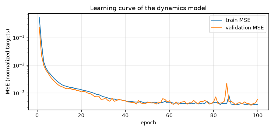
epoch    1 | train MSE 0.52619 | val MSE 0.23190
epoch   10 | train MSE 0.00231 | val MSE 0.00184
epoch   20 | train MSE 0.00131 | val MSE 0.00108
epoch   30 | train MSE 0.00073 | val MSE 0.00059
epoch   40 | train MSE 0.00052 | val MSE 0.00051
epoch   50 | train MSE 0.00047 | val MSE 0.00045
epoch   60 | train MSE 0.00044 | val MSE 0.00052
epoch   70 | train MSE 0.00042 | val MSE 0.00043
epoch   80 | train MSE 0.00046 | val MSE 0.00047
epoch   90 | train MSE 0.00038 | val MSE 0.00037
epoch  100 | train MSE 0.00038 | val MSE 0.00058
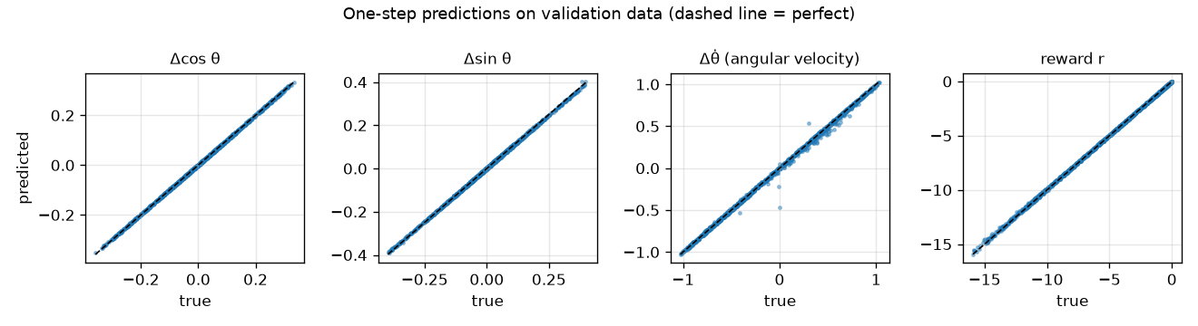
one-step accuracy on validation data:
  d_cos    RMSE 0.00161  (target std 0.1412)  R^2 0.99987
  d_sin    RMSE 0.00275  (target std 0.1470)  R^2 0.99965
  d_thdot  RMSE 0.02024  (target std 0.5686)  R^2 0.99873
  reward   RMSE 0.06770  (target std 4.0399)  R^2 0.99972
Standardized targets have variance 1, so a model that only outputs the mean has an MSE of about 1. After 100 epochs the MSE is around 0.0004, leaving only 0.04% of the variance unexplained. The validation loss tracks the training loss, so there is no sign of overfitting. The small fluctuations in validation loss come from Adam's uneven steps.
One-step prediction accuracy
\(y_i\) is the target, \(\hat y_i\) the prediction, and \(\bar y\) the mean of the targets.
\(\mathrm{RMSE} = \sqrt{\frac1N\sum_{i}(\hat y_i - y_i)^2}, \qquad R^2 = 1 - \frac{\sum_i (\hat y_i - y_i)^2}{\sum_i (y_i - \bar y)^2}\)
RMSE expresses the typical size of the error in the original units. The denominator of \(R^2\) is the error from guessing the single mean \(\bar y\) for everything; the numerator is the model's error. \(R^2 = 1\) means no error, and \(R^2 = 0\) means no better than guessing the mean.
- The RMSE of \(\Delta\dot\theta\) is 0.020, small compared with the validation targets' standard deviation of 0.569, giving \(R^2 = 0.9987\). The reward also has \(R^2 = 0.9997\). Without seeing the laws of physics, the model imitated the equation of motion almost exactly from data alone.
- Many of the outliers in \(\Delta\dot\theta\) occur at the moments when the angular velocity is clipped at \(\pm 8\). Among the 2,000 validation samples, the mean error at these 18 moments is 0.114, about 15 times that of the rest (0.008), and 8 of the 20 largest errors fall here. Clipping is a non-smooth rule, which is hard for an MLP to imitate.
- Figure: Four target-versus-prediction scatter plots on validation data; almost all points lie on the diagonal
Open-loop rollout
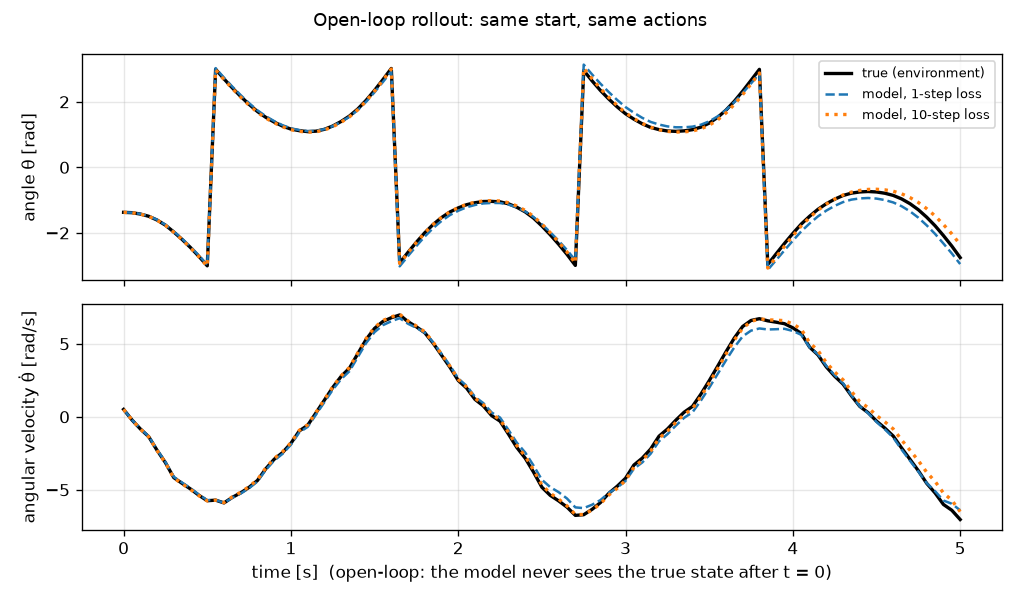
The purpose of a World Model is to imagine several steps ahead. Given only an initial observation \(o_0\) and an action sequence \(a_0, \dots, a_{H-1}\), feed the model's predictions back in as its inputs and roll forward \(H\) steps.
\(\hat o_1 = f_\theta(o_0, a_0),\quad \hat o_2 = f_\theta(\hat o_1, a_1),\quad \dots,\quad \hat o_H = f_\theta(\hat o_{H-1}, a_{H-1})\)
Because it never looks at the real observation again along the way, this is called an open-loop rollout. Restarting from the real observation at every step is closed-loop, that is, a method with feedback. The real observation is used only at the start, so any error that appears carries over to the next step.
@torch.no_grad()
def rollout(model, obs0, actions):
    """열린 고리(open-loop) 롤아웃: 시작 관측과 행동열만 주고, 모델의 예측을 다시 입력으로 넣어 H 스텝을 상상한다.

    obs0 (B, 3), actions (B, H, 1) → 예측 관측 (B, H+1, 3), 예측 보상 (B, H)
    진짜 관측은 시작할 때 한 번만 본다. 그 뒤로는 모델이 만든 '상상' 만 이어진다.
    """
    o = obs0
    obs_seq, rew_seq = [o], []
    for k in range(actions.shape[1]):
        o, r = model.predict(o, actions[:, k])
        obs_seq.append(o)
        rew_seq.append(r)
    return torch.stack(obs_seq, dim=1), torch.stack(rew_seq, dim=1)
The key is that in o, r = model.predict(o, actions[:, k]), o is overwritten by its own prediction. The batch dimension B computes many rollouts at once, and @torch.no_grad() turns off gradient tracking.
Rolling one validation episode open-loop for 100 steps (5 seconds), the prediction almost overlaps the real trajectory for the first 2 seconds or so; after that the one-step-loss model starts to drift away gradually.
Analyzing error accumulation
The tendency of a rollout to drift further from reality as it gets longer is called compounding error. Omitting actions, write the real environment as \(s_{k+1} = f(s_k)\), the model as \(\hat s_{k+1} = \hat f(\hat s_k)\), and the error after \(k\) steps as \(e_k = \lVert\hat s_k - s_k\rVert\). There are two assumptions.
- The one-step error is small: \(\lVert\hat f(s) - f(s)\rVert \le \varepsilon\) for all \(s\).
- The model is Lipschitz continuous: \(\lVert\hat f(s) - \hat f(s')\rVert \le L\,\lVert s - s'\rVert\) for all \(s, s'\). \(L\) is called the Lipschitz constant. If \(L \gt 1\), a small difference can grow by up to a factor of \(L\) per step; if \(L \lt 1\), it shrinks.
Recurrence
Subtract and add the same value \(\hat f(s_k)\) to split the error into "the part due to different starting points" and "the part due to the model being wrong," then apply the triangle inequality.
\(\begin{align} e_{k+1} &= \lVert\hat f(\hat s_k) - f(s_k)\rVert \\ &= \lVert\hat f(\hat s_k) - \hat f(s_k) + \hat f(s_k) - f(s_k)\rVert \\ &\le \lVert\hat f(\hat s_k) - \hat f(s_k)\rVert + \lVert\hat f(s_k) - f(s_k)\rVert \\ &\le L\,e_k + \varepsilon \end{align}\)
Upper bound
Substituting the recurrence repeatedly puts \(L^k\) in front of \(e_0\), followed by \(\varepsilon\) multiplied by \(L^{k-1}, \dots, L, 1\). The geometric series \(S = \sum_{j=0}^{k-1}L^j\) follows from \(LS - S = L^k - 1\).
\(\begin{align} e_k &\le L^k e_0 + \varepsilon\sum_{j=0}^{k-1}L^j \\ &= L^k e_0 + \varepsilon\,\frac{L^k - 1}{L - 1} \qquad (L \ne 1) \end{align}\)
A rollout starts from a real observation, so usually \(e_0 = 0\), and the bound is the one-step error \(\varepsilon\) times the amplification factor \(\frac{L^k-1}{L-1}\).
| Case | Bound | Meaning | Example: \(\varepsilon = 0.01\), \(k = 20\) |
| \(L \lt 1\) (model shrinks differences) | \(\varepsilon\frac{1 - L^k}{1-L} \lt \frac{\varepsilon}{1-L}\) | The error stays below a fixed value. | \(L = 0.9\): \(0.01\times\frac{1-0.9^{20}}{0.1} = 0.088\) |
| \(L = 1\) | \(k\,\varepsilon\) | The error grows in proportion to the number of steps. | \(0.01\times 20 = 0.2\) |
| \(L \gt 1\) (model can amplify differences) | \(\varepsilon\frac{L^k - 1}{L-1}\) | The error grows exponentially. | \(L = 1.1\): \(0.01\times\frac{1.1^{20}-1}{0.1} = 0.573\) |
\(1.1^{20} \approx 6.727\) and \(0.9^{20} \approx 0.122\). With the same one-step error, the bound after 20 steps for \(L = 1.1\) is more than 6 times that for \(L = 0.9\). Compounding error is especially severe not only when the model is bad, but when the world itself tends to amplify small differences.
How much the pendulum amplifies small differences
Near upright (\(\theta \approx 0\)), with \(\sin\theta \approx \theta\) and \(u = 0\), one step of semi-implicit Euler is as follows (\(15\Delta t = 0.75\)).
\(\dot\theta_{t+1} = \dot\theta_t + 0.75\,\theta_t, \qquad \theta_{t+1} = \theta_t + 0.05\,\dot\theta_{t+1} = 1.0375\,\theta_t + 0.05\,\dot\theta_t\)
\(\begin{pmatrix}\theta_{t+1}\\ \dot\theta_{t+1}\end{pmatrix} = A\begin{pmatrix}\theta_t\\ \dot\theta_t\end{pmatrix}, \qquad A = \begin{pmatrix}1.0375 & 0.05\\ 0.75 & 1\end{pmatrix}\)
The eigenvalues of \(A\) tell how many times, on average per step, a small difference grows over many steps.
\((1.0375 - \lambda)(1 - \lambda) - 0.05\times0.75 = 0 \ \Rightarrow\ \lambda^2 - 2.0375\lambda + 1 = 0 \ \Rightarrow\ \lambda = \frac{2.0375 \pm 0.3891}{2}\)
- Upright: \(\lambda_1 \approx 1.2133\), \(\lambda_2 \approx 0.8242\). Over the long run a small difference grows by about 1.21 times per step, and after 20 steps (1 second) by \(1.2133^{20} \approx 47.8\) times.
- Hanging down (\(\theta \approx \pi\)): the equation becomes \(\lambda^2 - 1.9625\lambda + 1 = 0\) with discriminant \(1.9625^2 - 4 \lt 0\), so both eigenvalues are complex with magnitude exactly 1. The difference neither grows nor shrinks; it oscillates.
- So even for the same model, the error grows fastest when imagining the moment the pendulum is being balanced upright. A well-trained model reproduces this property of the real pendulum faithfully.
- Eigenvalues and the Lipschitz constant are not the same thing. \(L\) is how much a difference can grow in one step in the worst case (measured with the ordinary vector length, about 1.48 for the \(A\) above and about 1.41 even when hanging down), while the eigenvalues give how much it actually grows on average per step over many steps. The bound \(\varepsilon\frac{L^k-1}{L-1}\) is a generous estimate; how fast the error actually grows over long rollouts is set by the eigenvalues.
Experiment
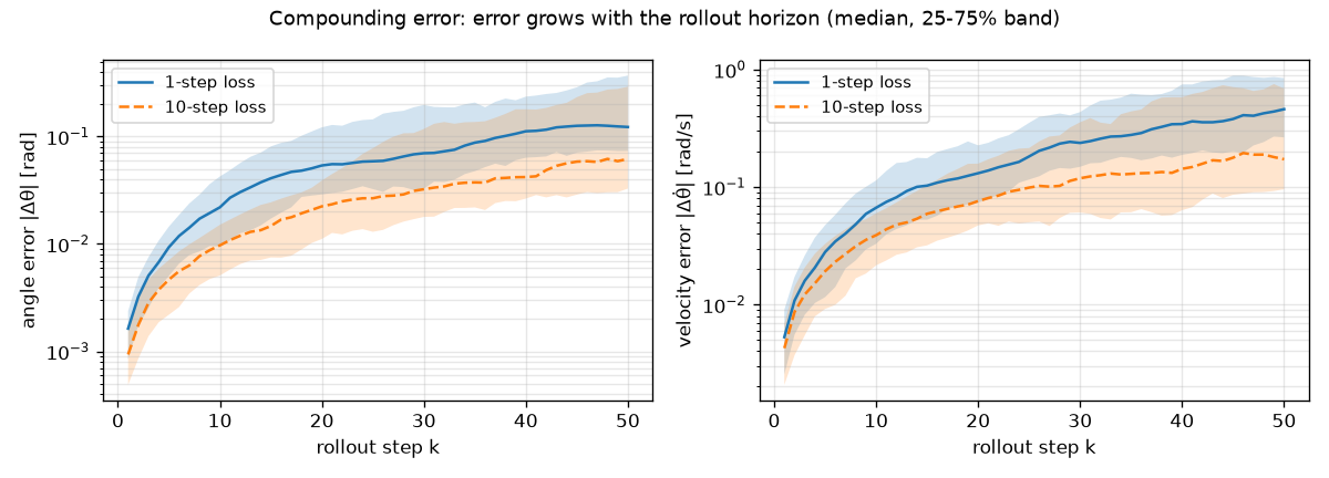
Starting from 300 random points in the validation episodes, roll out 50 steps with the recorded actions and measure the angle error \(\lvert\hat\theta - \theta\rvert\) and the angular velocity error at each step \(k\) (horizon_errors, horizon=50, n_starts=300). The angle is recovered with np.arctan2(obs[..., 1], obs[..., 0]), and the difference is wrapped into \([-\pi, \pi)\) with angle_normalize.
| Step \(k\) | One-step loss: angle [rad] | One-step loss: angular velocity | 10-step loss: angle [rad] | 10-step loss: angular velocity |
| 1 | 0.0016 | 0.0053 | 0.0009 | 0.0043 |
| 5 | 0.0093 | 0.0280 | 0.0047 | 0.0192 |
| 10 | 0.0219 | 0.0667 | 0.0097 | 0.0389 |
| 20 | 0.0538 | 0.1311 | 0.0224 | 0.0760 |
| 30 | 0.0700 | 0.2375 | 0.0323 | 0.1188 |
| 50 | 0.1228 | 0.4600 | 0.0618 | 0.1724 |
All values are medians. The one-step-loss model's angular velocity error is 0.0053 at step 1 but 0.46 at step 50, about 87 times larger. The 25–75% band is wide because the rate at which the error grows varies greatly with the starting point (especially whether the trajectory passes through the upright region). Chapter 7's planning looks about 25 steps ahead, so errors of this size are good enough for roughly correct imagination.
Reducing compounding error
Multi-step loss
When trained with a one-step loss, the model always receives the real observation as input, but during a rollout it receives its own prediction. It has never learned how to behave on slightly-off inputs. So rollouts are performed during training too, and their error is minimized directly.
\(\mathcal{L}_{k\text{-step}}(\theta) = \frac{1}{k}\sum_{j=1}^{k}\left[\ \big\lVert\, (\hat o_{t+j} - o_{t+j}) \oslash \sigma_{\Delta o} \big\rVert^2 + \Big(\frac{\hat r_{t+j-1} - r_{t+j-1}}{\sigma_r}\Big)^2\ \right]\)
\(\hat o_{t+j} = f_\theta(\hat o_{t+j-1}, a_{t+j-1}),\qquad \hat o_t = o_t\)
\(\oslash\) is element-wise division. Measuring the error in units of the standard deviation of \(\Delta o\) keeps it on the same scale as the one-step loss, and the code further averages by dividing by 4. With \(k = 1\) it equals the one-step loss. \(\hat o_{t+j}\) is the model's own prediction, and gradients also flow through that prediction. The information "a small error now becomes a big error a few steps later" reaches the weight updates for earlier steps.
    ow, aw, rw = (to_tensor(x, device) for x in make_windows(train_eps, k))
    scale_o, scale_r = model.out_std[:3], model.out_std[3]

    opt = torch.optim.Adam(model.parameters(), lr=lr)
    history = []
    n = len(ow)
    for epoch in range(1, epochs + 1):
        perm = torch.randperm(n, device=device)
        total = 0.0
        for i in range(0, n, batch_size):
            idx = perm[i : i + batch_size]
            o = ow[idx, 0]  # 진짜 관측은 첫 스텝에서만 쓴다
            loss = 0.0
            for j in range(k):
                o, r = model.predict(o, aw[idx, j])  # 예측을 다음 입력으로 (기울기도 그대로 흐른다)
                err_o = (o - ow[idx, j + 1]) / scale_o
                err_r = (r - rw[idx, j]) / scale_r
                loss = loss + (err_o.pow(2).sum(-1) + err_r.pow(2)).mean() / 4
            loss = loss / k
            opt.zero_grad()
            loss.backward()
            opt.step()
            total += loss.item() * len(idx)
make_windows(episodes, k) cuts episodes into windows of length \(k\), producing observations (N, k+1, 3), actions (N, k, 1), and rewards (N, k). The experiment in the text uses train_multistep(model_ms, train_eps, k=10, ...), with the same data, the same model size, and the same number of epochs.
- The median error after 50 steps drops from \(0.123 \to 0.062\) for the angle and \(0.46 \to 0.17\) for the angular velocity: about half for the angle and a little over a third for the angular velocity. The one-step error also decreased slightly.
- Each training step passes through the model \(k\) times, so training takes roughly \(k\) times as long.
Other methods
- Imagine briefly and check often: imagine only a short horizon and restart from the real observation at every step. This is what MPC in chapter 7 does.
- Know your uncertainty: if the model can express where it is unsure, imagination in those regions can be trusted less. This is the probabilistic ensemble in the second half of chapter 7.
- Collect more data where it is needed: acting with the model while collecting data increases data around the states actually visited (such as standing upright) (chapter 7).
- Predict in a good latent space: predicting in a compressed latent state instead of the observation simplifies what has to be predicted. This is the topic of chapters 8–12.
What this model is for
The trained model acts as a simulator of the pendulum and, unlike the real environment, allows the following.
- It can imagine hundreds of futures at once as a batch.
- Failure does not break the pendulum. This matters for a real robot.
- Being a neural network, it is differentiable and can be used for gradient-based optimization (Dreamer in chapter 12).
Chapter 7 makes the pendulum stand up through planning: it tries hundreds of action sequences in imagination and executes the best one.
Experiments to try
- Cut the data to 1/10 with
--episodes 5and see how the one-step and multi-step errors change. - Change the target in
make_inputs_targetsfromnext_obs - obstonext_obsand removeobs +frompredictso the model predicts the whole next state, then compare the one-step RMSE. - Turn off standardization in
set_normalizer(fix mean 0, standard deviation 1) and compare the learning curves. - Change
kintrain_multistepto 1, 3, and 20 and see how the error-by-horizon plot changes.
Summary
- The pendulum's equation of motion \(\ddot\theta = \frac{3g}{2l}\sin\theta + \frac{3}{ml^2}u\) follows from \(\tau = I\ddot\theta\), \(I = \frac13ml^2\), and the gravitational torque \(\frac{l}{2}mg\sin\theta\). The environment computes it with semi-implicit Euler in steps of \(\Delta t = 0.05\).
- Training a World Model is the regression problem \([o_t, a_t] \mapsto [o_{t+1}, r_t]\). Angles are handled as the seamless \((\cos\theta, \sin\theta)\).
- Standardization (mean 0 and standard deviation 1 per column) and predicting the change \(\Delta o\) make training easier. Statistics are computed from training data only.
- Minimizing MSE is equivalent to maximum likelihood training under Gaussian noise with fixed variance.
- An MLP with 34,180 parameters fit one step with \(R^2 \approx 0.999\), but errors accumulate in open-loop rollouts. The bound is \(e_k \le \varepsilon\frac{L^k - 1}{L - 1}\), which can grow exponentially when \(L \gt 1\); in practice the error grows fastest in unstable regions (the upright pendulum, eigenvalue about 1.21).
- Training with a multi-step loss cuts rollout error roughly in half. MPC, which imagines briefly and checks often, is covered in chapter 7.
Exercises
- One step of semi-implicit Euler
- With \(\theta_0 = \pi/2\), \(\dot\theta_0 = 0\), \(u = 0\), \(\Delta t = 0.05\): \(\ddot\theta_0 = 15\), \(\dot\theta_1 = 0.75\), and \(\theta_1 = 1.5708 + 0.0375 = 1.6083\). With explicit Euler, \(\theta_1 = 1.5708\) and the angle would not change.
- Moment of inertia of a rod rotating about its center
- \(I = \int_{-l/2}^{l/2} r^2\frac{m}{l}dr = \frac{m}{l}\cdot\frac13\left(\frac{l^3}{8} + \frac{l^3}{8}\right) = \frac{1}{12}ml^2\). This is \(\frac14\) of the value for rotation about an end; the closer the mass is to the axis, the easier it is to rotate.
- Angles at which the rod can be held still (\(\lvert u\rvert \le 2\))
- From \(15\sin\theta + 3u = 0\), \(u = -5\sin\theta\), so \(\lvert\sin\theta\rvert \le 0.4\) is required. Since \(\arcsin 0.4 \approx 0.4115\) rad \(\approx 23.6^\circ\), this means within about \(\pm 23.6^\circ\) of upright or within about \(\pm 23.6^\circ\) of hanging down (\(\lvert\theta\rvert \ge \pi - 0.4115\)). Angles in between have to be passed through by swinging.
- Undoing standardization (\(\mu = 2\), \(\sigma = 0.5\), \(\tilde y = -1.2\), MSE 0.0004 in the standardized space)
- \(y = -1.2\times0.5 + 2 = 1.4\). Errors scale as \(e = \tilde e\,\sigma\), so the RMSE in the original units is \(\sqrt{0.0004}\times0.5 = 0.01\).
- Error bound (\(\varepsilon = 0.005\), \(L = 1.2\), \(e_0 = 0\), 10 steps)
- \(e_{10} \le 0.005\times\frac{1.2^{10}-1}{1.2-1} = 0.005\times\frac{5.19}{0.2} \approx 0.13\). About 26 times the one-step error.
- Why rollout error grows even when the one-step error is small
- During training the input is always the real observation \(o_t\), while during a rollout it is the model's own slightly-wrong prediction \(\hat o_t\). The model never saw the distribution of these shifted inputs during training, so its accuracy there is not guaranteed, and the discrepancy grows as it carries over to the next step (a mismatch between the training and usage distributions, known as distribution shift). Multi-step loss reduces this gap by feeding the model's own predictions as inputs during training as well.
See also
- World Models:Tutorial
- World Models
- Reinforcement learning
- Maximum likelihood estimation
- Normal distribution
- Backpropagation
- PyTorch