WorldModels:Tutorial:05-ReinforcementLearning
lastmod 2026-11-18created 2026-11-172 edits
Reinforcement learning basics is chapter 5 of the World Model tutorial. A World Model is always used alongside an agent that is solving the problem of "how to act to collect as much reward as possible", so this chapter derives reinforcement learning, the mathematical framework for that problem, in the order MDP, return and discounting, value functions, and Bellman equations. It runs value iteration on a grid world, derives and trains a policy gradient method (REINFORCE), and then formulates the pendulum as a reinforcement learning problem to obtain the baseline scores the World Models of chapters 6 and 7 have to beat.
- Original: 05. Reinforcement Learning Basics
- Exercise code:
code/ch05_rl_basics.py(uses only numpy and matplotlib. Runpython ch05_rl_basics.pyin the same folder aswm_envs.py; the full run takes about 5–10 seconds, and--quickruns a reduced version. Figures are saved tofigures/) - Previous: 04. Deep Learning and PyTorch Basics / Next: 06. The First World Model
Agent and environment
Reinforcement learning (RL) is about learning by trial and error. An agent that chooses actions and an environment that responds to those actions repeat the same loop at every time step \(t = 0, 1, 2, \dots\). The agent observes the state \(s_t\) and picks an action \(a_t\) with its policy \(\pi(a \mid s)\), and the environment returns the next state \(s_{t+1}\) and a reward \(r_t\) according to its dynamics \(p(s' \mid s, a)\) and its reward function.
| Term | Meaning | In the pendulum |
| State \(s_t\) | Everything about the world right now | Angle and angular velocity \((\theta, \dot\theta)\) |
| Action \(a_t\) | What the agent chooses | Torque \(u \in [-2, 2]\) |
| Reward \(r_t\) | A single number saying how good the action was | \(-(\theta^2 + 0.1\dot\theta^2 + 0.001u^2)\) |
| Policy \(\pi\) | A rule mapping states to actions | E.g. "push against the tilt" |
| Episode | One run from start to finish | 200 steps (10 seconds) |
| Trajectory \(\tau\) | The record of one run \((s_0, a_0, r_0, s_1, a_1, r_1, \dots)\) | What |
There are two kinds of policies. A deterministic policy \(a = \mu(s)\) always produces the same action in the same state, while a stochastic policy \(a \sim \pi(a \mid s)\) samples actions from a probability distribution. Training mostly uses stochastic policies because they allow exploration and are easier to differentiate. For example, \(\pi(a \mid s) = \mathcal{N}(a;\ \mu_\psi(s), \sigma^2)\) is a policy that samples actions around a mean set by a neural network.
No teacher tells the agent the correct action. It only receives a score called the reward, and that score arrives late. To swing the pendulum up, the agent has to swing it the other way first, even if the reward gets worse for a while. The goal of reinforcement learning is to find a policy that maximizes the sum of future rewards, not the immediate reward.
Markov property and MDPs
The property that what happens next depends only on the present and not on the path taken to get there is called the Markov property.
\(p(s_{t+1} \mid s_t, a_t, s_{t-1}, a_{t-1}, \dots, s_0) = p(s_{t+1} \mid s_t, a_t)\)
For the pendulum, knowing \((\theta, \dot\theta)\) determines the next moment through the laws of physics, so this is a Markov state. The angle \(\theta\) alone does not tell which way the pendulum is turning, so it is not Markov. This distinction leads to the partial observability problem later in this chapter and to "memory" in chapters 9 and 11.
A decision problem that satisfies the Markov property is a Markov decision process (MDP), defined by five elements.
\(\text{MDP} = (\mathcal{S},\ \mathcal{A},\ p,\ r,\ \gamma)\)
- \(\mathcal{S}\) is the set of possible states, and \(\mathcal{A}\) is the set of possible actions.
- \(p(s' \mid s, a)\) is the transition probability. It corresponds to the rules of the world and is what a World Model tries to learn.
- \(r(s, a)\) (or \(r(s, a, s')\)) is the reward function.
- \(\gamma \in [0, 1)\) is the discount factor.
Factorizing the trajectory probability
Adding the initial state distribution \(\rho_0(s_0)\), we can write the probability of a trajectory under policy \(\pi\). Apply the product rule to the joint probability repeatedly in time order (the chain rule), then shorten the long conditions using the fact that the policy looks only at the current state and the environment looks only at the current state and action.
\(\begin{align} p(\tau) &= p(s_0)\, p(a_0 \mid s_0)\, p(s_1 \mid s_0, a_0)\, p(a_1 \mid s_0, a_0, s_1) \cdots \\ p_\pi(\tau) &= \rho_0(s_0)\prod_{t=0}^{T-1} \pi(a_t \mid s_t)\; p(s_{t+1} \mid s_t, a_t) \end{align}\)
The trajectory probability is the initial probability multiplied by the product of (policy probability × transition probability). This formula is the raw material for deriving the policy gradient.
Return and discounting
The discounted sum of the rewards received from time \(t\) onward is called the return \(G_t\).
\(G_t = r_t + \gamma r_{t+1} + \gamma^2 r_{t+2} + \cdots = \sum_{k=0}^{\infty} \gamma^k\, r_{t+k}\)
The discount factor \(\gamma\) sets how much a future reward is reduced when valued in the present. With \(\gamma = 0.9\), a reward of 1 one step later is worth 0.9 now, and one two steps later is worth 0.81. There are three reasons to discount.
- Math: the sum stays finite even in problems that never end.
- Uncertainty: predictions become less accurate the further they reach into the future. \(\gamma\) can also be read as the probability of surviving each step.
- Preference: for the same reward, receiving it sooner is better. This is what makes the agent take shortcuts in a grid world.
Geometric series and effective horizon
Multiplying \(S_n = 1 + \gamma + \cdots + \gamma^{n-1}\) by \(\gamma\) and subtracting cancels all the middle terms.
\(\begin{align} S_n - \gamma S_n &= 1 - \gamma^n \quad\Rightarrow\quad S_n = \frac{1 - \gamma^n}{1 - \gamma} \\ \sum_{k=0}^{\infty}\gamma^k &= \lim_{n\to\infty}\frac{1-\gamma^n}{1-\gamma} = \frac{1}{1-\gamma} \qquad (0 \le \gamma \lt 1) \end{align}\)
This is 10 for \(\gamma = 0.9\) and 100 for \(\gamma = 0.99\). If the reward always satisfies \(\vert r \vert \le R_{\max}\), then \(\vert G_t \vert \le \frac{R_{\max}}{1-\gamma}\), so the return is finite.
The \(k\) at which the weight \(\gamma^k\) of a reward \(k\) steps ahead drops to \(e^{-1} \approx 0.37\) is called the effective horizon. Since \(\gamma^k = e^{k\log\gamma}\), and for \(\gamma\) close to 1 the first-order Taylor approximation \(\log(1-x) \approx -x\) gives \(\log\gamma \approx -(1-\gamma)\), we get the following.
\(\gamma^k \approx e^{-k(1-\gamma)} = e^{-1} \quad\Longleftrightarrow\quad k \approx \frac{1}{1-\gamma}\)
For \(\gamma = 0.99\) this is about 100 steps (\(0.99^{100} = 0.366\), \(e^{-1} = 0.368\)). For the pendulum, with its 0.05-second time step, this means looking about 5 seconds ahead.
Recursive form of the return
Factoring a single \(\gamma\) out of the terms from the second one onward turns the part in parentheses into the return from \(t+1\).
\(G_t = r_t + \gamma\big(r_{t+1} + \gamma r_{t+2} + \gamma^2 r_{t+3} + \cdots\big) = r_t + \gamma\, G_{t+1}\)
This equation is the starting point for the Bellman equation, TD learning, and the λ-return in chapter 12. Thanks to the recursion, all returns can be computed in a single backward pass. With rewards \((1, 0, 0, 5)\) and \(\gamma = 0.9\), we get \(G_3 = 5\), \(G_2 = 4.5\), \(G_1 = 4.05\), and \(G_0 = 1 + 0.9 \times 4.05 = 4.645\), which matches the direct sum \(1 + 0.9^3 \times 5 = 4.645\).
def discounted_returns(rewards, gamma):
    """G_t = r_t + γ·G_{t+1} 를 뒤에서부터 계산한다. 결과는 rewards 와 길이가 같다."""
    G = np.zeros(len(rewards))
    running = 0.0  # 에피소드가 끝난 뒤의 리턴은 0
    for t in reversed(range(len(rewards))):
        running = rewards[t] + gamma * running
        G[t] = running
    return G
보상        : [1.0, 0.0, 0.0, 5.0]
리턴 G_t    : [4.645, 4.05, 4.5, 5.0]
G_0 직접 계산: 4.6450000000000005
γ=0.9: 보상 1 을 5000번 받은 리턴 = 10.0000,  1/(1−γ) = 10.0000
γ=0.99: 보상 1 을 5000번 받은 리턴 = 100.0000,  1/(1−γ) = 100.0000
The trailing digits of 4.6450000000000005 are a rounding error that comes from 0.9 not being exactly representable as a binary floating-point number.
Value functions
The return varies from run to run with the randomness of the policy and the environment, so its expected value is used to measure how good a state is.
\(\begin{align} V^\pi(s) &= \mathbb{E}_\pi\big[\,G_t \mid s_t = s\,\big] \\ Q^\pi(s, a) &= \mathbb{E}_\pi\big[\,G_t \mid s_t = s,\ a_t = a\,\big] \end{align}\)
The state value \(V^\pi(s)\) is the average return when starting from \(s\) and following \(\pi\), and the action value \(Q^\pi(s, a)\) is the average return when first taking \(a\) in \(s\) and following \(\pi\) afterward. For the pendulum, a state that is nearly upright and moving slowly has a \(V\) close to 0, while a state hanging down and spinning fast has a large negative value. Splitting cases by the first action with the law of total expectation gives the relationship between the two.
\(V^\pi(s) = \sum_a p(a_t = a \mid s_t = s)\;\mathbb{E}[G_t \mid s_t = s, a_t = a] = \sum_a \pi(a \mid s)\, Q^\pi(s, a)\)
The state value is the policy-weighted average of the action values.
Bellman expectation equation
Substituting the recursive form of the return into the definition of the value function turns an average over an infinite future into an equation that looks only one step ahead. This is the Bellman equation. The derivation uses three properties: linearity of expectation, the law of total expectation, and the Markov property.
\(\begin{align} V^\pi(s) &= \mathbb{E}_\pi\big[\, r_t + \gamma G_{t+1} \mid s_t = s \,\big] \\ &= \mathbb{E}_\pi[\, r_t \mid s_t = s\,] + \gamma\,\mathbb{E}_\pi[\, G_{t+1} \mid s_t = s\,] \\ &= \sum_a \pi(a\mid s)\sum_{s'} p(s'\mid s, a)\,\Big( r(s,a,s') + \gamma\,\mathbb{E}_\pi[\,G_{t+1} \mid s_t = s, a_t = a, s_{t+1} = s'\,]\Big) \end{align}\)
The second line uses linearity, \(\mathbb{E}[X + cY] = \mathbb{E}[X] + c\,\mathbb{E}[Y]\), and the third line splits cases by the first action \(a\) and the next state \(s'\). By the Markov property, once \(s_{t+1} = s'\) is known, everything after it is independent of the earlier states and actions, and since the policy does not change over time, the inner expectation is the value of \(s'\).
\(\mathbb{E}_\pi[\,G_{t+1} \mid s_t = s, a_t = a, s_{t+1} = s'\,] = \mathbb{E}_\pi[\,G_{t+1} \mid s_{t+1} = s'\,] = V^\pi(s')\)
\(V^\pi(s) = \sum_a \pi(a \mid s)\sum_{s'} p(s' \mid s, a)\,\big[\, r(s, a, s') + \gamma\, V^\pi(s')\,\big]\)
The value of the current state is the average of (current reward + discounted value of the next state). For \(Q\), the first action is fixed, so there is no outer average over \(\pi(a \mid s)\).
\(Q^\pi(s, a) = \sum_{s'} p(s' \mid s, a)\,\big[\, r(s, a, s') + \gamma\, V^\pi(s')\,\big] = \sum_{s'} p(s'\mid s,a)\Big[\, r + \gamma\sum_{a'}\pi(a'\mid s')\,Q^\pi(s', a')\Big]\)
Checking on a 2×3 grid
Take a grid with A, B, G in the top row and C, D, E in the bottom row, where G is the goal. The actions are up, down, left, and right, and moving into a wall leaves the agent where it is. Entering G gives a reward of +1 and ends the episode, every other move gives 0, \(\gamma = 0.9\), and moves are deterministic. With the policy "right in A, B, C, and D; up in E", every sum reduces to a single term.
\(\begin{align} V^\pi(B) &= r(B, \rightarrow, G) + \gamma V^\pi(G) = 1 + 0.9 \times 0 = 1, \qquad V^\pi(E) = 1 \\ V^\pi(A) &= 0 + 0.9\, V^\pi(B) = 0.9, \qquad V^\pi(D) = 0 + 0.9\, V^\pi(E) = 0.9 \\ V^\pi(C) &= 0 + 0.9\, V^\pi(D) = 0.81 \end{align}\)
G is a terminal state, so its value is 0, and each step further from the goal multiplies in one more \(\gamma\). These values are the same as the optimal values computed below.
Bellman optimality equation and value iteration
The value under the best policy \(\pi^\ast\) is the optimal value, \(V^\ast(s) = \max_\pi V^\pi(s)\) and \(Q^\ast(s,a) = \max_\pi Q^\pi(s,a)\). The optimal policy picks the best action at every moment, so the policy average in the Bellman expectation equation becomes a \(\max\). This is the Bellman optimality equation.
\(\begin{align} V^\ast(s) &= \max_a \sum_{s'} p(s' \mid s, a)\,\big[\, r(s,a,s') + \gamma\, V^\ast(s')\,\big] \\ Q^\ast(s, a) &= \sum_{s'} p(s' \mid s, a)\,\big[\, r(s,a,s') + \gamma \max_{a'} Q^\ast(s', a')\,\big] \end{align}\)
Once \(V^\ast\) is known, the optimal policy is to pick the action that maximizes \(\sum_{s'} p(s'\mid s,a)[r + \gamma V^\ast(s')]\). However, this computation requires the transition probability \(p(s'\mid s, a)\).
Value iteration
Value iteration repeatedly computes the right-hand side of the Bellman optimality equation and overwrites the left-hand side with it.
\(V_{k+1}(s) \leftarrow \max_a \sum_{s'} p(s' \mid s, a)\,\big[\, r(s,a,s') + \gamma\, V_k(s')\,\big], \qquad V_0(s) = 0\)
Running it by hand on the 2×3 grid (\(\gamma = 0.9\)) gives the following. The order is \((A, B, C, D, E)\), and G is always 0.
| Iteration | \((A, B, C, D, E)\) | Why it changed |
| \(V_0\) | \((0,\ 0,\ 0,\ 0,\ 0)\) | Initial values |
| \(V_1\) | \((0,\ 1,\ 0,\ 0,\ 1)\) | B moving right and E moving up both reach G, so \(1 + 0.9 \cdot 0 = 1\). For the rest, both the reward and \(V_0\) are 0. |
| \(V_2\) | \((0.9,\ 1,\ 0,\ 0.9,\ 1)\) | A moves right (to B), and D moves up (to B) or right (to E), giving \(0.9 \times 1\). C's neighbors A and D are still 0 in \(V_1\). |
| \(V_3\) | \((0.9,\ 1,\ 0.81,\ 0.9,\ 1)\) | \(V_3(C) = \max\{0.9 V_2(A),\ 0.9 V_2(D)\} = 0.81\) |
| \(V_4\) | \(V_4 = V_3 = V^\ast\) | Nothing changes any more, so it has converged. |
Information spreads one cell per iteration. The optimal policy is right in A and B, and up in C, D, and E (or another path with the same value). In the code, GridWorld.transitions(s, a) returns the environment's rules \(p(s', r \mid s, a)\) as a list [(probability, next state, reward), ...] (region grid in ch05_rl_basics.py).
def value_iteration(env, gamma, n_iters=1000, tol=1e-8, labels=None):
    """V_{k+1}(s) = max_a Σ_{s'} p(s'|s,a)·[r + γ·V_k(s')]  를 값이 더 바뀌지 않을 때까지 되풀이한다."""
    V = {s: 0.0 for s in env.states}  # V_0 = 0
    for k in range(n_iters):
        V_new = {}
        for s in env.states:
            if env.is_terminal(s):
                V_new[s] = 0.0  # 끝 칸 뒤에는 아무 보상도 없다
                continue
            q_values = [sum(p * (r + gamma * V[s2]) for p, s2, r in env.transitions(s, a)) for a in ACTIONS]
            V_new[s] = max(q_values)  # 가장 좋은 행동의 값
        delta = max(abs(V_new[s] - V[s]) for s in env.states)
        V = V_new
        if labels:  # 칸 이름을 주면 반복마다 값을 찍는다
            print(f"  반복 {k + 1}: " + "  ".join(f"{labels[s]}={V[s]:.3f}" for s in env.states))
        if delta < tol:
            break
    # 탐욕 정책: 각 칸에서 가장 큰 Q 를 주는 행동
    policy = {}
    for s in env.states:
        if not env.is_terminal(s):
            q = {a: sum(p * (r + gamma * V[s2]) for p, s2, r in env.transitions(s, a)) for a in ACTIONS}
            policy[s] = max(q, key=q.get)
    return V, policy, k + 1
The code's output matches the hand calculation, and the greedy policy is {'A': '→', 'B': '→', 'C': '↑', 'D': '↑', 'E': '↑'}.
5×5 slippery grid
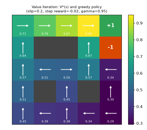
Now scale up to a 5×5 grid with walls (#), a goal G (+1), and a pit P (−1). With 20% probability the agent slips perpendicular to the intended direction (10% to each side, so transitions are stochastic), every move carries a penalty of \(-0.02\), and \(\gamma = 0.95\). The layout is ["....G", ".##.P", ".....", ".#.#.", "....."], with slip=0.2 and step_reward=-0.02.
  5×5 미끄러운 격자: 38번 반복 만에 수렴
   +0.707 +0.788 +0.866 +0.950   G
   +0.638   ##     ##   +0.667   P
   +0.567 +0.508 +0.501 +0.567 +0.341
   +0.508   ##   +0.445   ##   +0.295
   +0.445 +0.393 +0.388 +0.339 +0.294
The cell directly below the pit chooses the path that escapes to the left. Even so, it slips upward into the pit with 10% probability, so its value (0.34) is much lower than that of its left neighbor (0.57). The bottom-right corner cell heading back along the bottom row instead of moving up toward that cell is also the result of taking the risk of slipping into account.
Why value iteration converges
Each iteration shrinks the error from the solution by a factor of at most \(\gamma\) (a contraction). First we need the lemma \(\big\vert\max_a f(a) - \max_a g(a)\big\vert \le \max_a \vert f(a) - g(a)\vert\). Let \(a^\ast = \operatorname*{arg\,max}_a f(a)\). Since \(\max_a g \ge g(a^\ast)\),
\(\max_a f - \max_a g = f(a^\ast) - \max_a g \le f(a^\ast) - g(a^\ast) \le \vert f(a^\ast) - g(a^\ast)\vert \le \max_a \vert f(a) - g(a)\vert\)
and swapping \(f\) and \(g\) gives the inequality in the other direction, so the two combine into an absolute value. Now, subtracting the Bellman optimality equation from the definition of \(V_{k+1}\) cancels the reward \(r\).
\(\begin{align} \vert V_{k+1}(s) - V^\ast(s)\vert &= \Big\vert\max_a \sum_{s'} p\,[r + \gamma V_k(s')] - \max_a \sum_{s'} p\,[r + \gamma V^\ast(s')]\Big\vert \\ &\le \max_a \Big\vert\sum_{s'} p(s'\mid s,a)\,\gamma\,\big(V_k(s') - V^\ast(s')\big)\Big\vert \\ &\le \gamma \max_a \sum_{s'} p(s'\mid s,a)\,\big\vert V_k(s') - V^\ast(s')\big\vert \\ &\le \gamma \max_a \sum_{s'} p(s'\mid s,a)\, \|V_k - V^\ast\|_\infty = \gamma\, \|V_k - V^\ast\|_\infty \end{align}\)
The second line uses the lemma, the third the triangle inequality, and the fourth bounds each error by the maximum error \(\|V_k - V^\ast\|_\infty = \max_{s'}\vert V_k(s') - V^\ast(s')\vert\) and uses \(\sum_{s'} p(s'\mid s,a) = 1\). Since this holds for every \(s\), we get the following.
\(\|V_{k+1} - V^\ast\|_\infty \le \gamma\, \|V_k - V^\ast\|_\infty \quad\Rightarrow\quad \|V_k - V^\ast\|_\infty \le \gamma^k\, \|V_0 - V^\ast\|_\infty\)
For \(\gamma \lt 1\), \(\gamma^k \to 0\), so the values converge to \(V^\ast\) from any starting point.
Value iteration computed the optimal actions from the environment's rules \(p(s'\mid s,a)\) and reward \(r\) alone, without collecting a single data point. Using a model to decide on actions is called planning. In reality the rules are unknown, and learning them from data is what a World Model does. Chapter 6 and chapter 7 learn the pendulum's rules and plan inside the learned model.
Policy gradient: REINFORCE
The opposite approach does without the rules: it represents the policy itself as a neural network \(\pi_\psi\) and adjusts \(\psi\) directly in the direction that increases the return. The objective is the expected return.
\(J(\psi) = \mathbb{E}_{\tau \sim p_\psi}\big[ R(\tau) \big], \qquad R(\tau) = \sum_{t=0}^{T-1}\gamma^t r_t\)
Since this is a maximization problem, we use gradient ascent, \(\psi \leftarrow \psi + \eta\nabla_\psi J\). \(J\) can only be obtained by actually running the environment, and the environment is a black box that cannot be differentiated, but the log-derivative trick gives the gradient anyway.
\(\nabla_\psi \log p_\psi(\tau) = \frac{\nabla_\psi p_\psi(\tau)}{p_\psi(\tau)} \quad\Longleftrightarrow\quad \nabla_\psi p_\psi(\tau) = p_\psi(\tau)\,\nabla_\psi\log p_\psi(\tau)\)
Once a trajectory is fixed, \(R(\tau)\) does not depend on \(\psi\), so the derivative acts only on the probability, and applying the trick turns the result back into an expectation. That expectation can be estimated by sampling trajectories and averaging.
\(\begin{align} \nabla_\psi J &= \nabla_\psi \sum_\tau p_\psi(\tau)\,R(\tau) = \sum_\tau \nabla_\psi p_\psi(\tau)\,R(\tau) \\ &= \sum_\tau p_\psi(\tau)\,\nabla_\psi\log p_\psi(\tau)\,R(\tau) = \mathbb{E}_{\tau\sim p_\psi}\big[\, R(\tau)\,\nabla_\psi \log p_\psi(\tau)\,\big] \end{align}\)
Taking the log of the factorized trajectory probability splits it into three terms. The initial distribution \(\rho_0\) and the environment's rules \(p\) do not depend on \(\psi\), so their derivatives are 0.
\(\begin{align} \log p_\psi(\tau) &= \log\rho_0(s_0) + \sum_{t}\log\pi_\psi(a_t\mid s_t) + \sum_t \log p(s_{t+1}\mid s_t, a_t) \\ \nabla_\psi \log p_\psi(\tau) &= 0 + \sum_t \nabla_\psi\log\pi_\psi(a_t\mid s_t) + 0 \end{align}\)
The environment terms vanish, leaving the policy gradient theorem.
\(\nabla_\psi J = \mathbb{E}_{\tau\sim p_\psi}\Big[\, R(\tau)\sum_{t=0}^{T-1}\nabla_\psi \log\pi_\psi(a_t\mid s_t)\,\Big]\)
All it needs are trajectories from actual rollouts and the gradient of the policy's log probability. It does not need the environment's rules, so it is model-free. In words: "raise the probability of the actions taken in trajectories that had high returns."
Baselines: reducing variance
The estimate above is unbiased but very noisy. The tool for reducing the noise is the fact that the expected value of the score function \(\nabla\log\pi\) is 0.
\(\mathbb{E}_{a\sim\pi_\psi(\cdot\mid s)}\big[\nabla_\psi\log\pi_\psi(a\mid s)\big] = \sum_a \pi_\psi(a\mid s)\,\frac{\nabla_\psi \pi_\psi(a\mid s)}{\pi_\psi(a\mid s)} = \nabla_\psi \sum_a \pi_\psi(a\mid s) = \nabla_\psi\, 1 = 0\)
So subtracting from the return a value \(b(s_t)\) that does not depend on the action \(a_t\), called a baseline, leaves the expected gradient unchanged.
\(\mathbb{E}[(G - b(s))\nabla\log\pi] = \mathbb{E}[G\,\nabla\log\pi] - b(s)\cdot\mathbb{E}[\nabla\log\pi] = \mathbb{E}[G\,\nabla\log\pi] - 0\)
By the same logic, an action at time \(t\) cannot affect rewards received before it, so the return from that point on, \(G_t\), can be used instead of \(R(\tau)\). The REINFORCE used in practice is as follows (the factor of \(\gamma^t\) is usually ignored in practice).
\(\nabla_\psi J \approx \frac{1}{N}\sum_{\text{trajectories}}\ \sum_{t}\big(G_t - b(s_t)\big)\,\nabla_\psi\log\pi_\psi(a_t \mid s_t)\)
A good choice of baseline is the state's average return \(V^\pi(s_t)\). Then \(G_t - b(s_t)\) means "how much better than usual", so actions that did better than usual are pushed up and actions that did worse are pushed down.
Score function of a softmax policy
When there are only a few actions, keep a logit \(\psi_{s,a}\) for each state and build the policy with a softmax. This is the same calculation as the cross-entropy gradient in chapter 4, with only the sign flipped.
\(\begin{align} \log\pi(a\mid s) &= \psi_{s,a} - \log\sum_{b'} e^{\psi_{s,b'}} \\ \frac{\partial}{\partial\psi_{s,b}}\log\pi(a\mid s) &= \mathbf{1}[b = a] - \frac{e^{\psi_{s,b}}}{\sum_{b'}e^{\psi_{s,b'}}} = \mathbf{1}[b=a] - \pi(b\mid s) \end{align}\)
The logit of the chosen action goes up by \((1 - \pi)\), and every other action goes down by its own probability. grad_log_pi in the code implements this formula.
Exercise: corridor
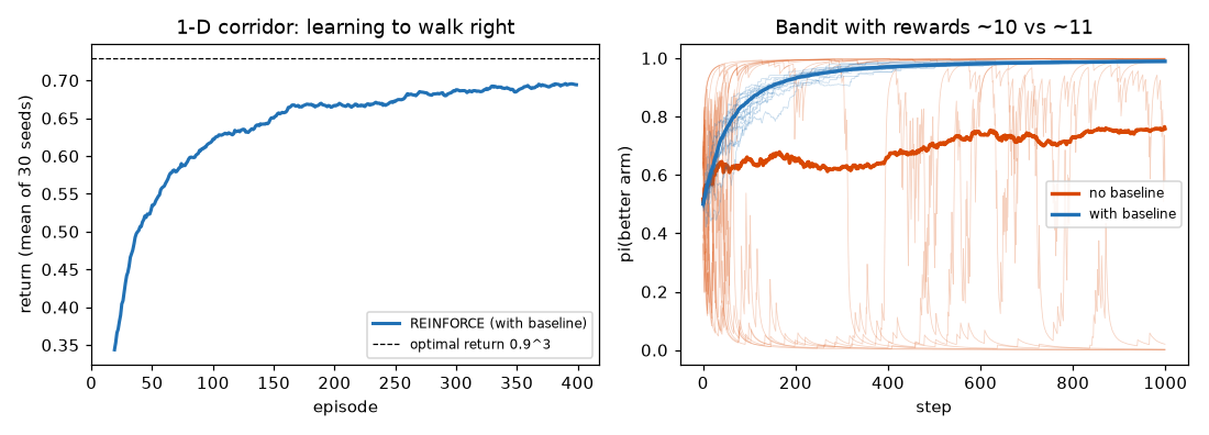
In a one-dimensional corridor of cells 0–4, the agent starts in cell 0 and receives +1 on reaching cell 4 (0 if it does not get there within 15 steps). There are two actions, left and right, with \(\gamma = 0.9\), a learning rate of 0.1, 400 episodes, and 30 seeds. The optimal behavior is to move right four times and receive a return of \(0.9^3 = 0.729\). The environment is in region corridor.
def run_episode(env, logits, rng):
    """정책 π(a|s) = softmax(logits[s]) 로 에피소드 하나를 돈다."""
    s, done = env.reset(), False
    states, actions, rewards = [], [], []
    while not done:
        a = rng.choice(2, p=softmax(logits[s]))
        s2, r, done = env.step(a)
        states.append(s), actions.append(a), rewards.append(r)
        s = s2
    return states, actions, rewards


def grad_log_pi(logits, s, a):
    """∇_logits log π(a|s). 소프트맥스 정책이면 (원-핫(a) − π(·|s)) 가 s 행에만 생긴다."""
    g = np.zeros_like(logits)
    g[s] = -softmax(logits[s])
    g[s, a] += 1.0
    return g


def reinforce(n_episodes, gamma, lr, use_baseline, seed):
    rng = np.random.default_rng(seed)
    env = Corridor(rng)
    logits = np.zeros((env.n_states, env.n_actions))  # 처음엔 왼쪽 · 오른쪽 반반
    V = np.zeros(env.n_states)  # 기준선 b(s): 상태별 리턴의 이동 평균
    returns = []
    for _ in range(n_episodes):
        states, actions, rewards = run_episode(env, logits, rng)
        G = discounted_returns(rewards, gamma)  # 각 시각의 리턴 G_t
        grad = np.zeros_like(logits)
        for s, a, g_t in zip(states, actions, G):
            b = V[s] if use_baseline else 0.0
            grad += (g_t - b) * grad_log_pi(logits, s, a)  # (G_t − b)·∇log π(a_t|s_t)
            if use_baseline:
                V[s] += 0.1 * (g_t - V[s])  # 기준선도 조금씩 리턴 쪽으로
        logits += lr * grad  # 경사 '상승': 리턴을 키우는 방향
        returns.append(G[0])
    return np.array(returns), logits
grad += (g_t - b) * grad_log_pi(...) is \(\sum_t (G_t - b(s_t))\nabla\log\pi\), and logits += lr * grad is the gradient ascent step. For simplicity, the code updates the baseline V[s] in the middle of an episode. Strictly speaking, it should be updated after the episode ends so that the baseline is fully independent of that episode's actions.
To confirm that the baseline only reduces the noise and leaves the mean unchanged, sample 4,000 episodes from the initial (50/50) policy and compare the mean and variance of the gradient estimates (region variance; the baseline is the Monte Carlo average of the returns for each state).
Exercise: bandit
In a two-armed slot machine (a bandit), arm 0 pays a reward with mean 10 and arm 1 a reward with mean 11 (standard deviation 1). Every reward contains a large common value of 10, so without a baseline, whichever arm is pulled gets its probability raised sharply. The run uses 1,000 steps, a learning rate of 0.05, and 50 seeds.
def bandit_reinforce(steps, lr, use_baseline, seed, means=(10.0, 11.0)):
    """팔 두 개짜리 밴딧. 보상 ~ N(10, 1) 또는 N(11, 1). 모든 보상에 큰 공통 값(약 10)이 섞여 있다."""
    rng = np.random.default_rng(seed)
    logits = np.zeros(2)
    b = None  # 기준선: 받은 보상의 이동 평균
    history = []
    for _ in range(steps):
        p = softmax(logits)
        a = rng.choice(2, p=p)
        r = rng.normal(means[a], 1.0)
        if b is None:
            b = r
        g = -p
        g[a] += 1.0  # ∇ log π(a)
        logits += lr * (r - (b if use_baseline else 0.0)) * g
        b += 0.05 * (r - b)
        history.append(softmax(logits)[1])  # 좋은 팔(1)을 고를 확률
    return np.array(history)
Results
| Experiment | Without baseline | With baseline |
| Corridor gradient mean (cell 0, right) | +0.0825 | +0.0806 |
| Corridor gradient variance, summed | 0.5944 | 0.3862 |
| Corridor mean return over the last 50 episodes (optimal 0.729) | 0.690 | 0.695 |
| Bandit mean \(\pi(\text{good arm})\) after 1,000 steps | 0.758 | 0.989 |
| Bandit seeds stuck on the bad arm | 22% | 0% |
After training with the baseline in the corridor, \(\pi(\text{right} \mid s)\) in cells 0–3 is [0.872, 0.949, 0.957, 0.948]. The gradient means agree within sampling noise, and the variance dropped by 35%. In a problem like the corridor, where rewards are only 0 and 1, the learning curves differ little, but when the rewards share a large common value, as in the bandit, the policy easily locks onto whichever arm it happened to pull first if there is no baseline. The pendulum's rewards are always negative, roughly \(-16.3\) to \(0\), so it falls into this case.
Actor-critic, advantage, and TD error
Using \(V^\pi(s)\) as the baseline requires knowing its value, so the value function is also represented as a neural network \(v_\xi(s)\) and learned alongside the policy. The policy \(\pi_\psi\) is called the actor, the value function \(v_\xi\) the critic, and this structure actor-critic. The actor and critic are exactly what Dreamer in chapter 12 learns in imagination.
- The actor \(\pi_\psi(a \mid s)\) sends an action \(a\) to the environment.
- The environment returns a reward \(r\) and the next state \(s'\).
- The critic outputs \(v(s)\) and \(v(s')\), which form the TD error \(\delta = r + \gamma v(s') - v(s)\).
- The actor adjusts its action probabilities using \(\delta\) (\(\propto \delta\, \nabla \log \pi\)), and the critic adjusts its value predictions to reduce \(\delta^2\).
\(Q^\pi(s,a) - V^\pi(s)\) is called the advantage \(A^\pi(s, a)\). It measures how much better this action is than the average for this state, and \(G_t - V(s_t)\) is an estimate of it. Estimating it from a single step gives the TD (temporal difference) error.
\(\delta_t = r_t + \gamma V^\pi(s_{t+1}) - V^\pi(s_t)\)
\(\begin{align} \mathbb{E}[\delta_t \mid s_t, a_t] &= \mathbb{E}[\, r_t + \gamma V^\pi(s_{t+1}) \mid s_t, a_t\,] - V^\pi(s_t) \\ &= \sum_{s'}p(s'\mid s_t,a_t)\,[\,r + \gamma V^\pi(s')\,] - V^\pi(s_t) \\ &= Q^\pi(s_t, a_t) - V^\pi(s_t) = A^\pi(s_t, a_t) \end{align}\)
Each individual TD error is noisy, but on average it equals the advantage. Because it uses a one-step reward plus the critic's guess instead of the actual return \(G_t\), which mixes in all the randomness of the long future, its variance is lower; in exchange, it is biased to the extent that the critic is wrong. The λ-return in chapter 12 is a way to blend the two.
The critic learns to move toward the target \(y_t = r_t + \gamma\,v_\xi(s_{t+1})\) by minimizing the MSE \(\big(y_t - v_\xi(s_t)\big)^2\). If the target moves along with the critic, training becomes unstable, so no gradient flows into the target. This is called stop-gradient and is written \(\operatorname{sg}(y_t)\).
Even so, the target is produced by the critic itself, so every update to the critic also moves the target (a "moving target"). To reduce this, a copy of the critic is made that follows the original critic only occasionally (or very slowly), and the target \(y_t\) is computed with this slow copy. This is the target network, a device DQN (Mnih et al., 2015) used to stabilize training. The "slow critic" in chapter 12 is the same idea.
Reparameterization gradient
REINFORCE treats the environment as a black box, so it cannot use derivative information such as "how much does the reward go up if the torque is increased slightly". A World Model is a neural network and therefore differentiable, so it yields more accurate gradients. In the simplest example, sample an action \(a \sim \mathcal{N}(\mu, 1)\) and receive the reward \(f(a) = a^2\). Then \(J(\mu) = \mathbb{E}[a^2] = \mu^2 + 1\), and the true gradient is \(\nabla_\mu J = 2\mu\). There are two ways to estimate it from samples.
- Score function (REINFORCE) estimator
- Since \(\nabla_\mu \log\mathcal{N}(a;\mu,1) = \nabla_\mu\Big(-\tfrac{(a-\mu)^2}{2} - \tfrac{1}{2}\log 2\pi\Big) = a - \mu\), the estimator is \(\hat{g}_{\text{SF}} = f(a)\,(a - \mu) = a^2(a-\mu)\). It does not differentiate \(f\).
- Reparameterization estimator
- Writing \(a = \mu + \epsilon,\ \epsilon\sim\mathcal{N}(0,1)\) moves the randomness into \(\epsilon\), which does not depend on \(\mu\), and makes \(a\) a differentiable function of \(\mu\). The estimator is \(\hat{g}_{\text{RP}} = \frac{\partial f(\mu+\epsilon)}{\partial \mu} = 2(\mu + \epsilon) = 2a\). This is the key technique behind the VAE in chapter 8.
Both are unbiased (\(\mathbb{E}[\epsilon] = \mathbb{E}[\epsilon^3] = 0\), \(\mathbb{E}[\epsilon^2] = 1\)).
\(\mathbb{E}[\hat{g}_{\text{RP}}] = 2\mu,\qquad \mathbb{E}[\hat{g}_{\text{SF}}] = \mathbb{E}[(\mu+\epsilon)^2\epsilon] = \mathbb{E}[\mu^2\epsilon + 2\mu\epsilon^2 + \epsilon^3] = 0 + 2\mu + 0 = 2\mu\)
The difference is in the variance. At \(\mu = 1\), \((1+\epsilon)^4\epsilon^2 = \epsilon^2 + 4\epsilon^3 + 6\epsilon^4 + 4\epsilon^5 + \epsilon^6\), and the even moments of the standard normal distribution, \(\mathbb{E}[\epsilon^{2k}] = (2k-1)(2k-3)\cdots 1\), give \(\mathbb{E}[\epsilon^4] = 3\) and \(\mathbb{E}[\epsilon^6] = 15\), so the expectation is \(1 + 0 + 18 + 0 + 15 = 34\).
\(\operatorname{Var}[\hat{g}_{\text{RP}}] = 4\operatorname{Var}[\epsilon] = 4,\qquad \operatorname{Var}[\hat{g}_{\text{SF}}] = \mathbb{E}[(1+\epsilon)^4\epsilon^2] - 2^2 = 34 - 4 = 30\)
The reparameterization estimator has 7.5 times less variance, so it needs 7.5 times fewer samples to reach the same accuracy.
import numpy as np

rng = np.random.default_rng(0)
mu, n = 1.0, 1_000_000
eps = rng.standard_normal(n)
a = mu + eps                       # a ~ N(μ, 1)

score = a**2 * (a - mu)            # f(a) · ∇_μ log N(a; μ, 1)
pathwise = 2 * a                   # ∇_a f(a) · ∂a/∂μ

print("참값 2μ      :", 2 * mu)
print("점수 함수    : 평균 %.3f, 분산 %.2f" % (score.mean(), score.var()))
print("재매개변수화 : 평균 %.3f, 분산 %.2f" % (pathwise.mean(), pathwise.var()))
The real environment cannot be differentiated through, so one has to rely on score function estimates or on a separately learned value function. When imagining inside a learned World Model, however, state → action → next state → reward are all neural networks, so the return can be differentiated directly with respect to the policy parameters. This reparameterization gradient is what Dreamer uses to learn behavior in imagination for continuous actions.
Partial observability: POMDPs and belief states
From chapter 8 on, the agent sees only a 64×64 image \(o_t\), not the true state. The image shows the angle but not the angular velocity. A problem in which observations reveal only part of the state is a partially observable Markov decision process (POMDP).
\(\text{POMDP} = (\mathcal{S}, \mathcal{A}, p, r, \gamma,\ \mathcal{O},\ p(o \mid s))\)
It adds a set of observations \(\mathcal{O}\) and an observation model \(p(o \mid s)\) to the MDP. Because the state is unknown, the agent has to carry around "a probability distribution over the current state" built from its observations and actions so far. This is the belief state \(b_t(s) = p(s_t = s \mid o_{1:t}, a_{1:t-1})\). The belief is updated with Bayes' theorem every time a new observation arrives (a Bayes filter).
\(b_{t+1}(s') = \frac{p(o_{t+1} \mid s_{t+1}=s', o_{1:t}, a_{1:t})\; p(s_{t+1}=s' \mid o_{1:t}, a_{1:t})}{p(o_{t+1} \mid o_{1:t}, a_{1:t})}\)
An observation depends only on the state at that moment, so the first term of the numerator reduces to \(p(o_{t+1} \mid s')\). The second term is marginalized over the current state \(s\). The next state depends only on the current state and action, and the action \(a_t\) was chosen by looking at the history, so it does not change the belief about the current state.
\(p(s_{t+1}=s' \mid o_{1:t}, a_{1:t}) = \sum_s p(s' \mid s, a_t)\; p(s_t = s \mid o_{1:t}, a_{1:t-1}) = \sum_s p(s' \mid s, a_t)\, b_t(s)\)
The denominator is a constant that does not depend on \(s'\), so we write the update as a proportionality.
\(b_{t+1}(s') \propto \underbrace{p(o_{t+1}\mid s')}_{\text{correct with the observation}}\ \underbrace{\sum_s p(s'\mid s, a_t)\, b_t(s)}_{\text{predict with the model}}\)
The two steps are predicting the next state with the transition model and strengthening the belief in states that agree with the new observation. For the pendulum, the velocity can be estimated from the change in angle between two images (\(\dot\theta \approx (\theta_t - \theta_{t-1})/\Delta t\)), and the belief update generalizes this probabilistically over many images. In real problems the state space is too large to compute this sum exactly, so a World Model uses a neural-network summary instead. The hidden state \(h_t\) of the MDN-RNN in chapter 9 and the latent state \((h_t, z_t)\) of the RSSM in chapter 11 are learned belief states, and the RSSM's structure closely mirrors the two steps "predict → correct".
Model-free vs. model-based, and Dyna
| Model-free | Model-based | |
| What is learned | The policy and values, learned directly from experience. | First learns a model of the environment, \(p_\theta(s'\mid s,a)\) and \(r_\theta\) (= World Model), then plans or learns a policy inside it. |
| Examples | REINFORCE, actor-critic, DQN, PPO, SAC | Value iteration (when the model is known), Dyna, PETS (chapter 7), World Models (chapter 10), PlaNet (chapter 11), Dreamer (chapter 12), MuZero (chapter 13) |
| Pros | Unaffected by model error. Simple to implement. | Data efficiency: each real experience updates the model, and the model can generate unlimited imagined experience. Enables planning and reuse for new goals. |
| Cons | Requires a very large number of interactions with the environment (millions of steps). | Model error: errors compound (chapter 6), and the policy can exploit the places where the model is wrong, known as model exploitation (chapters 7 and 10). Complex to implement. |
A classic idea bridging the two is Richard Sutton's Dyna (Dyna architecture, Sutton, 1990–1991). It updates both the model and the value function from real experience, then updates the value function several more times using simulated experience generated by the model.
되풀이:
    1. 실제 환경에서 행동 a 를 하고 (s, a, r, s') 를 얻는다
    2. 이 실제 경험으로 가치 함수(또는 정책)를 고친다          ← 모델 프리 학습
    3. 이 경험으로 모델 p_θ(s'|s,a), r_θ 를 고친다             ← World Model 학습
    4. n 번 되풀이:                                            ← 상상(계획)
         지금까지 본 상태 s 와 행동 a 를 하나 고르고
         모델로 가상의 (r̂, ŝ') 를 만들어
         그 가상 경험으로 가치 함수를 고친다
Step 3 is World Model learning, and step 4 is practicing in a dream. The rest of the tutorial can be read as growing this skeleton: chapter 6 implements step 3 (model learning), chapter 7 implements step 4 as planning (MPC), and chapters 10 and 12 implement step 4 as policy learning.
The pendulum as a reinforcement learning problem
| Element | Pendulum environment ( |
| State \(s\) | \((\theta, \dot\theta)\). A Markov state. |
| Observation \(o\) | Chapters 6 and 7: \([\cos\theta, \sin\theta, \dot\theta]\) (same information as the state, so an MDP). From chapter 8: a 64×64 image (the velocity is not visible, so a POMDP). |
| Action \(a\) | Torque \(u \in [-2, 2]\) (continuous action) |
| Transition \(p\) | Deterministic physics \(\ddot\theta = \frac{3g}{2l}\sin\theta + \frac{3}{ml^2}u\) (derived in chapter 6), Euler integration with \(\Delta t = 0.05\), angular velocity clipped at \(\pm 8\). |
| Initial state | \(\theta\) uniformly random in \([-\pi, \pi]\), \(\dot\theta\) uniformly random in \([-1, 1]\) |
| Reward \(r\) | \(-(\theta^2 + 0.1\dot\theta^2 + 0.001u^2)\) (\(\theta\) wrapped to \([-\pi, \pi)\)). The range is about \([-16.3,\ 0]\): the worst case is \(\pi^2 + 0.1\cdot 8^2 + 0.001\cdot 2^2 \approx 16.27\) |
| Episode | Cut off at 200 steps (there is no terminal state). The evaluation score is the undiscounted sum of rewards over the 200 steps. |
| Discount factor | Usually \(\gamma = 0.99\) during training (effective horizon of about 100 steps = 5 seconds) |
wm_envs.Pendulum implements the same physics as Gym Pendulum-v1 directly in numpy (\(m = l = 1\), \(g = 10\)). The reward is computed from the state before the move, and the velocity is updated first and then used to update the angle (semi-implicit Euler). The interface is obs = env.reset() and obs, reward, done = env.step(action). The torque limit of 2 is weaker than the maximum torque gravity exerts on the rod, \(mgl/2 = 5\), so the rod cannot be lifted in one go; the agent has to swing back and forth to build up energy and then balance it at the top.
A hand-crafted policy: energy pumping + PD control
As a point of comparison, we build a policy that someone who knows the physics could write. The key insight is that applying torque in the direction of rotation increases the energy. Multiply both sides of the equation of motion by the rod's moment of inertia \(I = \frac{ml^2}{3}\), and differentiate the energy with respect to time.
\(\begin{align} I\ddot\theta &= \frac{mgl}{2}\sin\theta + u \\ E &= \tfrac{1}{2}I\dot\theta^2 + \tfrac{mgl}{2}\cos\theta \\ \frac{dE}{dt} &= I\dot\theta\,\ddot\theta - \frac{mgl}{2}\sin\theta\,\dot\theta = \dot\theta\,\Big(I\ddot\theta - \frac{mgl}{2}\sin\theta\Big) = \dot\theta\, u \end{align}\)
\(E\) is the sum of the rotational kinetic energy and the potential energy (center-of-mass height \(\frac{l}{2}\cos\theta\), with \(\theta = 0\) at the very top). At rest at the top, \(E = \frac{mgl}{2} = 5\); at rest at the bottom, it is \(-5\). If \(\dot\theta u \gt 0\), the energy increases.
The policy has two parts. Unless the rod is near the top (\(\cos\theta \gt 0.9\), about ±25°), it pushes in the direction of rotation in proportion to the gap from the target energy of 5 (energy pumping). Near the top, PD control \(u = -K_p\theta - K_d\dot\theta\) (\(K_p = 10\), \(K_d = 2\)) keeps it balanced. Near the top, approximating \(\sin\theta \approx \theta\) gives
\(\ddot\theta \approx 15\theta + 3u = 15\theta - 30\theta - 6\dot\theta = -15\theta - 6\dot\theta\)
which is stable motion with a spring (restoring force \(-15\theta\)) and friction (\(-6\dot\theta\)). Because the torque is clipped to ±2, this equation holds exactly only in the narrow range \(\vert 10\theta + 2\dot\theta \vert \le 2\); outside it, balance is achieved because energy pumping delivers the rod to the top at a suitable speed.
def random_policy(obs, rng):
    return rng.uniform(-2.0, 2.0, size=1)


def zero_policy(obs, rng):
    return np.zeros(1)


def energy_pd_policy(obs, rng=None, k_energy=1.0, kp=10.0, kd=2.0, switch_cos=0.9):
    """손으로 만든 정책: 아래에서는 에너지를 펌프질하고, 위 근처에서는 PD 제어로 균형을 잡는다."""
    cos_th, sin_th, thdot = obs
    th = np.arctan2(sin_th, cos_th)  # [-π, π], 0 = 똑바로 선 자세
    if cos_th > switch_cos:  # 위에서 약 ±25° 안: PD 제어
        u = -kp * th - kd * thdot  # 기울어진 반대쪽으로, 도는 반대쪽으로 민다
    else:  # 그 밖: 에너지 펌핑
        inertia = 1.0 / 3.0  # I = m l² / 3  (m = l = 1)
        energy = 0.5 * inertia * thdot**2 + 5.0 * np.cos(th)  # E = ½Iθ̇² + (mgl/2)·cos θ
        direction = 1.0 if thdot >= 0 else -1.0  # 도는 방향으로 밀면 에너지가 늘어난다 (dE/dt = θ̇·u)
        u = k_energy * (5.0 - energy) * direction  # 목표 에너지 mgl/2 = 5 와의 차이만큼
    return np.clip(np.array([u]), -2.0, 2.0)
Baseline scores
We measure the undiscounted 200-step reward sum over 100 episodes with random starts (region evaluate).
| Policy | Mean | Std. dev. | Min | Max |
| random | −1233.7 | 298.4 | −1867.0 | −754.2 |
| zero torque | −1239.6 | 367.3 | −1898.6 | −494.8 |
| energy + PD | −182.5 | 106.3 | −368.2 | −0.0 |
Starting from hanging straight down, the hand-crafted policy swings back and forth twice to build up energy, raises the rod at about 3.5 seconds, and holds it upright until the end. The random policy and the do-nothing policy stay near the bottom.
- Figure: Rod height over time when starting from the bottom, and the average return of the three policies
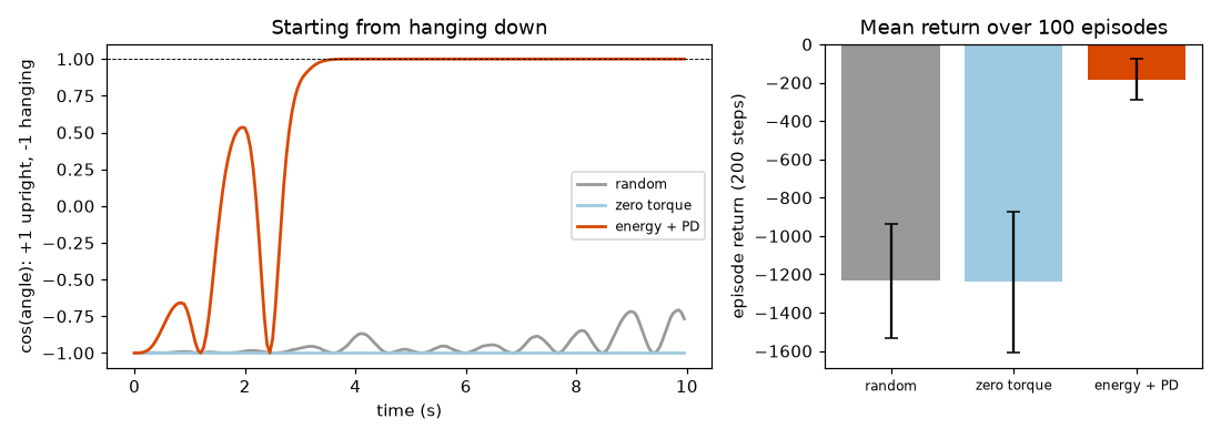
The random policy scores about −1234, and the policy written by someone who knows the physics scores about −183. The hand-crafted policy could only be written with knowledge of the energy equation. The goal of chapters 6 and 7 is to approach this score (around −200) without knowing the laws of physics, by learning a World Model only from randomly collected data and planning inside it.
Summary
- In an MDP \((\mathcal{S}, \mathcal{A}, p, r, \gamma)\), the Markov property lets the trajectory probability factorize as \(\rho_0\prod_t \pi(a_t\mid s_t)\,p(s_{t+1}\mid s_t,a_t)\).
- The return is \(G_t = \sum_k \gamma^k r_{t+k} = r_t + \gamma G_{t+1}\). \(\sum\gamma^k = \frac{1}{1-\gamma}\), and the effective horizon is \(\approx \frac{1}{1-\gamma}\).
- The Bellman expectation equation \(V^\pi(s) = \sum_a\pi\sum_{s'}p\,[r + \gamma V^\pi(s')]\) follows from linearity, total expectation, and the Markov property. For the optimal case, a \(\max\) replaces the average.
- Value iteration converges because it shrinks the error by a factor of at most \(\gamma\) each time. However, it needs the transition probability \(p\) (= the model).
- In the policy gradient \(\nabla J = \mathbb{E}[\sum_t (G_t - b)\nabla\log\pi]\), the log-derivative trick makes the environment terms vanish. A baseline reduces the variance without changing the mean.
- The expected value of the TD error \(\delta = r + \gamma V(s') - V(s)\) is the advantage. Actor-critic uses it to learn the policy and the values together.
- Inside a differentiable World Model, the reparameterization gradient gives gradients with much lower variance (chapter 12).
- Seeing only images makes the problem a POMDP. A belief update predicts with the model and then corrects with the observation, and RNNs and RSSMs replace it with a learned summary.
- The pendulum baseline scores are −1234 for the random policy and −183 for the hand-crafted policy.
Review questions
- 1. \(G_0, G_1, G_2\) for \(\gamma = 0.5\) and rewards \((2, 0, 4)\)
- \(G_2 = 4\), \(G_1 = 0 + 0.5 \times 4 = 2\), and \(G_0 = 2 + 0.5 \times 2 = 3\). As a check, \(2 + 0.5^2 \times 4 = 3\).
- 2. The return and effective horizon for \(\gamma = 0.95\) when the reward is \(-1\) at every step forever
- The return is \(-1 \times \frac{1}{1 - 0.95} = -20\), and the effective horizon is \(\frac{1}{0.05} = 20\) steps (\(0.95^{20} \approx 0.358\)).
- 3. \(V^\ast(C)\) on the 2×3 grid when \(\gamma\) is changed to \(0.5\)
- From C, reaching the goal takes at least 3 moves (e.g. C → A → B → G), and the +1 comes on the last move, so \(V^\ast(C) = \gamma^2 \times 1 = 0.25\).
- 4. Why the transition probability \(p(s'\mid s,a)\) does not appear in the REINFORCE gradient
- The log of the trajectory probability splits into \(\log\rho_0 + \sum\log\pi_\psi + \sum\log p\), and \(\rho_0\) and \(p\) do not depend on \(\psi\), so their derivatives are 0. The environment is used only to sample trajectories.
- 5. Why subtracting a baseline \(b(s)\) does not change the expectation, and whether the baseline may depend on the action
- Since \(\mathbb{E}_{a\sim\pi}[\nabla\log\pi(a\mid s)] = \nabla\sum_a\pi = \nabla 1 = 0\), the term multiplied by \(b(s)\) has an expectation of 0. If \(b\) depends on \(a\), it cannot be pulled out of the expectation, the argument breaks down, and in general a bias is introduced.
- 6. What an agent that sees a single pendulum image needs in order to know the direction of rotation
- It needs the history of previous observations (at least one more image) and actions. Because this is a POMDP in which observations show only part of the state, the agent has to carry a belief state (or an RNN hidden state) that summarizes the history.
See also
- World Models:Tutorial
- World Models
- Reinforcement learning
- Markov decision process
- Policy
- Q-learning
- Softmax
- Bayes' theorem