WorldModels:Tutorial:04-DeepLearningBasics
lastmod 2026-11-18created 2026-11-172 edits
Deep learning and PyTorch basics is Chapter 4 of the World Model tutorial. A world model is a neural network that implements "a function that takes a state and an action and returns the next state", so this chapter derives the tools for training that network (derivatives, gradient descent, and backpropagation) from their definitions. It works through backpropagation in a two-layer network by hand with concrete numbers and confirms that PyTorch autograd produces the same values. It then covers Adam, overfitting and regularization, tensors and the training loop, and convolutional neural networks (CNNs), and ends by training a CNN that reads the angle from a pendulum image. Every model from Chapter 6 onward uses this chapter's training loop unchanged.
- Original: 04. Deep Learning and PyTorch Basics
- Exercise code:
code/ch04_basics.py(runpython ch04_basics.pyin the same folder aswm_envs.py. A full run takes about 3–6 minutes on 4 laptop CPU threads, most of it the final CNN training.--quicktakes about 10 seconds. Figures are saved tofigures/.) - Previous: 03. Information Theory and KL Divergence / Next: 05. Reinforcement Learning Basics
A neural network is a function with parameters
In \(y = wx + b\), values such as \(w\) and \(b\) that determine the shape of the function are called parameters. A neural network is a function with anywhere from thousands to billions of parameters. All the parameters together are written \(\theta\), and the function the network represents is written \(f_\theta\).
\(\hat{y} = f_\theta(x)\)
Training means looking at data \(\{(x_i, y_i)\}\) and finding a \(\theta\) that brings \(f_\theta(x_i)\) close to \(y_i\). Learning from data in which every input is paired with a correct answer is called supervised learning. A loss function \(L(\theta)\) measures "how close" as a single number, and the most common one is the mean squared error (MSE).
\(L(\theta) = \frac{1}{N} \sum_{i=1}^{N} \big(f_\theta(x_i) - y_i\big)^2, \qquad \theta^\ast = \operatorname*{arg\,min}_\theta L(\theta)\)
The reason for using squares comes from Gaussian maximum likelihood in Chapter 2. The world model in Chapter 6 uses the same framework; the only difference is that the input \(x\) is (state, action) and the target \(y\) is the next state.
The training loop (Figure 4-1 in the original) repeats the following four steps thousands of times.
- Forward pass: feed the data \(x\) into the model \(f_\theta\) to get a prediction \(\hat{y}\).
- Loss: compare \(\hat{y}\) with the target \(y\) and compute \(L\).
- Backpropagation: compute the gradient \(\nabla_\theta L\), that is, which way to adjust each parameter so that \(L\) decreases.
- Update: \(\theta \leftarrow \theta - \eta \nabla_\theta L\).
In PyTorch code, a step that clears the previous step's gradients is added at the front, making five steps. This chapter explains why steps 3 and 4 work.
Derivatives
Definition
The derivative \(f'(x)\) is the factor by which \(f\) changes when \(x\) changes by a tiny amount, that is, the slope of the graph.
\(f'(x) = \frac{df}{dx} = \lim_{h \to 0} \frac{f(x+h) - f(x)}{h}\)
For \(f(x) = x^2\) at \(x = 3\), the average slope is 6.1, 6.01, and 6.001 for \(h = 0.1,\ 0.01,\ 0.001\), approaching 6. Algebraically:
\(\begin{align} \frac{(x+h)^2 - x^2}{h} &= \frac{x^2 + 2xh + h^2 - x^2}{h} = 2x + h \\ f'(x) &= \lim_{h \to 0} (2x + h) = 2x \end{align}\)
Differentiation rules
Training neural networks requires five rules.
| Rule | Formula | Derivation sketch |
| Constant multiple, sum | \((c\,f)' = c\,f'\), \((f + g)' = f' + g'\) | In the numerator of the definition, pull \(c\) out or split the \(f\) and \(g\) parts. Example: \((3x^2 + x)' = 6x + 1\). |
| Power | \((x^n)' = n x^{n-1}\) | By the binomial theorem, \((x+h)^n = x^n + n x^{n-1} h + \binom{n}{2} x^{n-2} h^2 + \cdots + h^n\). After subtracting \(x^n\) and dividing by \(h\), every term except the first, \(n x^{n-1}\), is still multiplied by \(h\) and vanishes in the limit. The rule also holds for negative and fractional \(n\) (\((x^{-1})' = -x^{-2}\)). |
| Product | \((fg)' = f'g + fg'\) | Subtract and add \(f(x)g(x+h)\) in the numerator, group it as \(\big(f(x+h) - f(x)\big)g(x+h) + f(x)\big(g(x+h) - g(x)\big)\), then divide by \(h\) and take the limit. |
| Exponential, logarithm | \((e^x)' = e^x\), \((\log x)' = 1/x\) | \(e \approx 2.71828\) is the number for which \(\lim_{h \to 0} \frac{e^h - 1}{h} = 1\). Then \(\frac{e^{x+h} - e^x}{h} = e^x \cdot \frac{e^h - 1}{h} \to e^x\). For the logarithm, differentiate both sides of \(y = \log x \Leftrightarrow x = e^y\) with respect to \(x\) to get \(1 = e^y \frac{dy}{dx}\), so \(\frac{dy}{dx} = \frac{1}{e^y} = \frac{1}{x}\). |
| Chain rule | \(\frac{dy}{dx} = \frac{dy}{du} \cdot \frac{du}{dx}\) | See below. |
The chain rule gives the derivative of a composite function \(y = f(g(x))\). A neural network is a composite function built from stacked layers, so this one rule is, in effect, backpropagation. Let the intermediate value be \(u = g(x)\), with \(\Delta u = g(x + h) - g(x)\) and \(\Delta y = f(u + \Delta u) - f(u)\). Then
\(\frac{\Delta y}{h} = \frac{\Delta y}{\Delta u} \cdot \frac{\Delta u}{h} \quad\Longrightarrow\quad \frac{dy}{dx} = f'(u) \cdot g'(x)\)
(This assumes \(\Delta u \ne 0\). A rigorous proof handles the case \(\Delta u = 0\) separately, but the result is the same.) Multiply the derivative of the outer function by the derivative of the inner function. Rates of change multiply, just as with meshed gears: if the second gear turns 3 times for each turn of the first, and the third turns 2 times for each turn of the second, the third gear turns \(3 \times 2 = 6\) times.
Example: for \(y = (3x + 1)^2\), \(u = 3x + 1\) and \(y = u^2\), so \(\frac{dy}{dx} = 2u \cdot 3 = 6(3x+1)\), which is 24 at \(x = 1\). Numerical check: \((4.003^2 - 16)/0.001 = 24.009\).
Partial derivatives and the gradient vector
With several parameters, differentiating with respect to one of them while holding the rest fixed gives the partial derivative \(\partial\). For the loss on a single data point \((x, y) = (2, 5)\), \(L(w, b) = (2w + b - 5)^2\):
\(\frac{\partial L}{\partial w} = 2(2w + b - 5) \cdot 2, \qquad \frac{\partial L}{\partial b} = 2(2w + b - 5) \cdot 1\)
\(\nabla L = \begin{pmatrix} \partial L / \partial w \\ \partial L / \partial b \end{pmatrix} = \begin{pmatrix} 4(2w + b - 5) \\ 2(2w + b - 5) \end{pmatrix} \;\overset{w=b=0}{=}\; \begin{pmatrix} -20 \\ -10 \end{pmatrix}\)
The vector of partial derivatives is the gradient \(\nabla L\). Each component of \(\nabla_\theta L\) says how much the loss grows when that parameter is increased by a tiny amount. If it is positive, the parameter should be decreased; if negative, increased. The gradient vector points in the direction in which the loss increases most steeply.
Gradient descent
Moving against the gradient reduces the loss
Gradient descent repeats the following single line. \(\eta\) is the learning rate, a small positive number that sets how far to move at each step.
\(\theta \leftarrow \theta - \eta \, \nabla_\theta L(\theta)\)
Why the loss decreases is explained by a first-order Taylor approximation.
\(\begin{align} L(\theta + \Delta) &\approx L(\theta) + \sum_j \frac{\partial L}{\partial \theta_j}\Delta_j = L(\theta) + \nabla L \cdot \Delta \\ \Delta = -\eta \nabla L \;&\Longrightarrow\; L(\theta_{\text{new}}) \approx L(\theta) - \eta\, \lVert\nabla L\rVert^2 \;\le\; L(\theta) \end{align}\)
\(\lVert\nabla L\rVert^2\) is a sum of squares and therefore non-negative, so if \(\eta\) is small enough for the approximation to hold, the loss always decreases. When the gradient is 0, the parameters stop moving (a candidate minimum).
The geometric meaning of the dot product also shows that, for a fixed step length \(\lVert\Delta\rVert = c\), the direction that reduces the loss the most is \(-\nabla L\).
\(\nabla L \cdot \Delta = \lVert\nabla L\rVert\,\lVert\Delta\rVert \cos\alpha, \qquad \min_{\lVert\Delta\rVert = c} \nabla L \cdot \Delta = -\lVert\nabla L\rVert\, c \quad (\alpha = 180^\circ)\)
The original tutorial compares this to walking down a fog-covered mountain, feeling only the slope under your feet. If your stride (the learning rate) is too small, you barely descend; if it is too large, you overshoot the valley and climb the opposite slope.
Upper bound on the learning rate
For a bowl-shaped loss \(L(w) = \frac{a}{2}w^2\) (\(a \gt 0\)), \(a\) is the curvature. Since \(L'(w) = aw\),
\(w_{k+1} = (1 - \eta a)\, w_k \quad\Longrightarrow\quad w_k = (1 - \eta a)^k\, w_0\)
\(w_k \to 0 \iff \vert 1 - \eta a \vert \lt 1 \iff 0 \lt \eta \lt \frac{2}{a}\)
- If \(\eta \gt 2/a\), \(w\) flips sign and grows (divergence).
- If \(\eta = 1/a\), it reaches the minimum in one step.
- With several parameters, the curvature differs by direction, and the steepest direction sets the upper bound on the learning rate.
Linear regression by hand
Fit a line \(\hat{y} = wx + b\) to three points \((1, 3), (2, 5), (3, 7)\) with MSE (the answer is \(y = 2x + 1\)). With residuals \(e_i = w x_i + b - y_i\), the chain rule gives
\(\frac{\partial L}{\partial w} = \frac{2}{N}\sum_i e_i x_i, \qquad \frac{\partial L}{\partial b} = \frac{2}{N}\sum_i e_i\)
Starting from \(w = b = 0\) with \(\eta = 0.05\) gives the following.
| Step | \(w\) | \(b\) | Residuals \(e\) | Loss | \(\partial L/\partial w\) | \(\partial L/\partial b\) |
| 0 | 0 | 0 | \((-3, -5, -7)\) | \(83/3 \approx 27.6667\) | \(\frac{2}{3}(-34) \approx -22.6667\) | \(\frac{2}{3}(-15) = -10\) |
| 1 | 1.1333 | 0.5 | \((-1.3667, -2.2333, -3.1)\) | 5.4885 | \(-10.0889\) | \(-4.4667\) |
| 2 | 1.6378 | 0.7233 | 1.0897 | \(-4.4874\) | \(-2.0022\) |
After 2000 steps, \(w = 2.0000\), \(b = 1.0000\), and the loss is \(1.43 \times 10^{-24}\). The code below does the same computation in numpy; the derived gradient formulas become the two lines dw and db.
def linreg_gradient_descent(x, y, lr=0.05, steps=2000, verbose_steps=3):
    """ŷ = w·x + b 를 MSE 로 맞춘다. 기울기는 손으로 유도한 식을 그대로 쓴다.

    L  = (1/N) Σ (w·x_i + b − y_i)²
    ∂L/∂w = (2/N) Σ (w·x_i + b − y_i)·x_i
    ∂L/∂b = (2/N) Σ (w·x_i + b − y_i)
    """
    w, b = 0.0, 0.0  # 시작점: 아무것도 모르는 상태
    n = len(x)
    history = []  # (w, b, loss)
    for step in range(steps + 1):
        y_hat = w * x + b  # 예측 (N,)
        err = y_hat - y  # 잔차 (N,)
        loss = np.mean(err**2)  # MSE
        history.append((w, b, loss))
        if step < verbose_steps:
            dw = 2.0 / n * np.sum(err * x)
            db = 2.0 / n * np.sum(err)
            print(f"  step {step}: w={w:.4f} b={b:.4f} loss={loss:.4f}  dL/dw={dw:.4f} dL/db={db:.4f}")
        if step == steps:
            break
        dw = 2.0 / n * np.sum(err * x)  # ∂L/∂w
        db = 2.0 / n * np.sum(err)  # ∂L/∂b
        w = w - lr * dw  # 기울기 반대 방향으로 한 스텝
        b = b - lr * db
    return w, b, np.array(history)
The loss after 200 steps at different learning rates is as follows.
| Learning rate | Loss after 200 steps |
| 0.01 | 5.556e-04 (slow) |
| 0.05 | 1.154e-05 |
| 0.17 | 8.211e-11 |
| 0.19 | 1.601e+19 (diverges) |
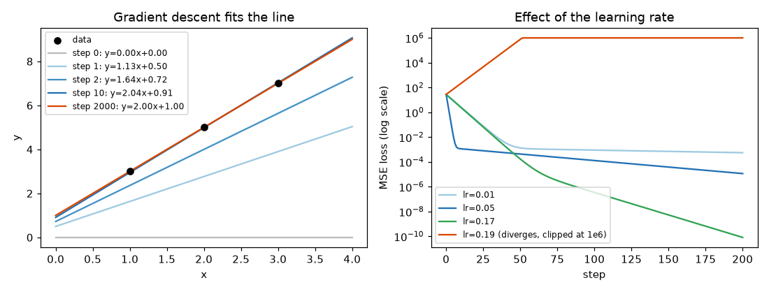
The boundary sits at 0.18 because of the eigenvalues of the Hessian matrix (the table of second derivatives). Since \(\frac{\partial^2 L}{\partial w^2} = \frac{2}{N}\sum x_i^2 = \frac{28}{3} \approx 9.333\), \(\frac{\partial^2 L}{\partial b^2} = 2\), and \(\frac{\partial^2 L}{\partial w \partial b} = \frac{2}{N}\sum x_i = 4\),
\(H = \begin{pmatrix} 9.333 & 4 \\ 4 & 2 \end{pmatrix},\qquad \det(H - \lambda I) = \lambda^2 - 11.333\lambda + 2.667 = 0\)
\(\lambda = \frac{11.333 \pm 10.853}{2} \approx 11.093,\ 0.240\)
Along each eigenvector, the loss is a bowl of the form \(\frac{\lambda}{2}w^2\), so each eigenvalue is the curvature in that direction. The steepest direction has curvature 11.093, so convergence requires \(\eta \lt 2/11.093 \approx 0.180\). 0.17 is inside this bound and 0.19 is outside. The flattest direction has a small curvature of 0.240, so at \(\eta = 0.01\) the parameters move along it very slowly.
Activation functions and stacking layers
Linear layers and nonlinearity
A linear layer (fully-connected layer) transforms an input \(x \in \mathbb{R}^{n}\) using a weight matrix \(W \in \mathbb{R}^{m \times n}\) and a bias \(b \in \mathbb{R}^m\).
\(z = W x + b, \qquad z_j = \sum_{i=1}^{n} W_{ji}\, x_i + b_j\)
Stacking only linear layers, no matter how many, is equivalent to a single linear layer.
\(y = W_2 (W_1 x + b_1) + b_2 = W' x + b', \qquad W' = W_2 W_1,\ b' = W_2 b_1 + b_2\)
So an activation function is inserted between layers and applied element-wise, as in \(h = \sigma(Wx + b)\). The universal approximation theorem states that, with enough hidden neurons, such a network can approximate any continuous function on a bounded interval as closely as desired.
Sigmoid, tanh, ReLU
| Function | Formula | Range | Derivative | Use |
| Sigmoid | \(\sigma(z) = \frac{1}{1 + e^{-z}}\) | 0 to 1 | \(\sigma(z)(1 - \sigma(z))\), maximum 0.25 (at \(z = 0\)) | Outputs that are probabilities or brightness values between 0 and 1. Used only in the last layer. |
| tanh | \(\tanh(z) = \frac{e^z - e^{-z}}{e^z + e^{-z}}\) | -1 to 1 | \(1 - \tanh^2(z)\), maximum 1 (at \(z = 0\)) | Its outputs average near 0, which suits hidden layers. Common in RNNs (Chapter 9). |
| ReLU | \(\max(0, z)\) | 0 or greater | 1 if \(z \gt 0\), 0 if \(z \lt 0\) (usually set to 0 at \(z = 0\)) | The cheapest to compute, and its derivative does not shrink on the positive side, making it the default for deep networks. |
Numerical examples: \(\sigma(0) = 0.5\), \(\sigma(2) \approx 0.881\), \(\sigma(-2) \approx 0.119\), \(\sigma'(2) \approx 0.881 \times 0.119 \approx 0.105\). For sigmoid and tanh, the derivative approaches 0 when \(\vert z \vert\) is large (saturation).
The derivative of the sigmoid follows from applying the chain rule to \(\sigma(z) = (1 + e^{-z})^{-1}\).
\(\begin{align} \sigma'(z) &= -(1 + e^{-z})^{-2} \cdot (-e^{-z}) = \frac{1}{1 + e^{-z}} \cdot \frac{e^{-z}}{1 + e^{-z}} \\ \frac{e^{-z}}{1 + e^{-z}} &= \frac{(1 + e^{-z}) - 1}{1 + e^{-z}} = 1 - \sigma(z) \\ \sigma'(z) &= \sigma(z)\,\big(1 - \sigma(z)\big) \end{align}\)
The derivative needs only \(\sigma(z)\), which the forward pass has already computed. tanh is a stretched and shifted sigmoid.
\(\begin{align} 2\sigma(2z) - 1 &= \frac{1 - e^{-2z}}{1 + e^{-2z}} = \frac{e^z - e^{-z}}{e^z + e^{-z}} = \tanh(z) \\ \tanh'(z) &= 2\,\sigma'(2z)\cdot 2 = 4s(1 - s), \qquad s = \sigma(2z) \\ 1 - \tanh^2 &= 1 - (2s - 1)^2 = 4s - 4s^2 = 4s(1-s) \end{align}\)
Vanishing gradient (vanishing gradient): the sigmoid's derivative is at most 0.25, so with 10 stacked layers the gradient can shrink to \(0.25^{10} \approx 10^{-6}\) during backpropagation, and almost none of it reaches the early layers. This is why hidden layers mostly use ReLU. The problem comes up again with RNNs (Chapter 9).
Backpropagation: a two-layer network by hand
Backpropagation is not new mathematics. It applies the chain rule step by step starting from the output and reuses intermediate results.
The network and its numbers
| Part | Formula | Value |
| Input | \(x = (x_1, x_2)\) | \((1.0,\ 0.5)\) |
| Layer 1 (2 hidden units) | \(z = W_1 x + b_1\), \(h = \sigma(z)\) | \(W_1 = \begin{pmatrix} 0.5 & -0.4 \\ 0.3 & 0.8 \end{pmatrix}\), \(b_1 = (0.1,\ -0.2)\) |
| Layer 2 (1 output) | \(\hat{y} = w_2 \cdot h + b_2\) (no activation function) | \(w_2 = (1.2,\ -0.7)\), \(b_2 = 0.05\) |
| Loss | \(L = (\hat{y} - y)^2\) | Target \(y = 1.0\) |
Forward pass
\(\begin{align} z_1 &= 0.5 \cdot 1.0 + (-0.4)\cdot 0.5 + 0.1 = 0.4, \qquad z_2 = 0.3 \cdot 1.0 + 0.8 \cdot 0.5 - 0.2 = 0.5 \\ h_1 &= \sigma(0.4) = \frac{1}{1 + 0.670320} = 0.598688, \qquad h_2 = \sigma(0.5) = \frac{1}{1 + 0.606531} = 0.622459 \\ \hat{y} &= 1.2 \times 0.598688 - 0.7 \times 0.622459 + 0.05 = 0.332704 \\ L &= (0.332704 - 1)^2 = (-0.667296)^2 = 0.445284 \end{align}\)
Backward pass
There are 9 parameters (4 in \(W_1\), 2 in \(b_1\), 2 in \(w_2\), and \(b_2\)). The computation runs backward from the output, and each step multiplies the value just obtained on its right by one local derivative.
| Step | Quantity | Formula (local derivative) | Value |
| 1 | \(\partial L/\partial \hat{y}\) | \(2(\hat{y} - y)\) | \(-1.334593\) |
| 2 | \(\partial L/\partial w_{2,j}\) | \(\frac{\partial L}{\partial \hat{y}} \cdot h_j\) | \((-0.799004,\ -0.830730)\) |
| 3 | \(\partial L/\partial b_2\) | \(\frac{\partial L}{\partial \hat{y}} \cdot 1\) | \(-1.334593\) |
| 4 | \(\partial L/\partial h_j\) | \(\frac{\partial L}{\partial \hat{y}} \cdot w_{2,j}\) | \((-1.601511,\ 0.934215)\) |
| 5 | \(\sigma'(z_j) = h_j(1 - h_j)\) | Reuses forward-pass values | \((0.240261,\ 0.235004)\) |
| 6 | \(\partial L/\partial z_j\) | \(\frac{\partial L}{\partial h_j} \cdot h_j(1 - h_j)\) | \((-0.384780,\ 0.219544)\) |
| 7 | \(\partial L/\partial W_{1,ji}\) | \(\frac{\partial L}{\partial z_j} \cdot x_i\) (outer product of \(\partial L/\partial z\) and \(x\)) | \(\begin{pmatrix} -0.384780 & -0.192390 \\ 0.219544 & 0.109772 \end{pmatrix}\) |
| 8 | \(\partial L/\partial b_1\) | \(\frac{\partial L}{\partial z} \cdot 1\) | \((-0.384780,\ 0.219544)\) |
The \(\partial L/\partial h_j\) in step 4 is not a parameter gradient, but it is needed to pass the gradient further left. In step 5, the sigmoid's local gradient is at most 0.25, so the gradient shrinks to roughly a quarter.
The structure of backpropagation comes down to three points.
- Each node does one thing: it passes (the gradient received from the right) × (this node's local derivative) to the left.
- The local derivatives reuse values computed in the forward pass (\(h_j\), \(x_i\)). That is why forward-pass values are kept in memory.
- \(\partial L/\partial \hat{y}\), computed once at the output, is reused in the gradient of every parameter. This is why backpropagation costs only about 2–3 times as much as the forward pass, even with billions of parameters.
One update step
Updating all 9 parameters with \(\eta = 0.1\) gives, for example, \(w_{2,1} = 1.2 - 0.1 \times (-0.799004) = 1.279900\), \(W_{1,11} = 0.538478\), and \(b_2 = 0.183459\). Running the forward pass again gives \(\hat{y} = 0.599293\) and \(L = 0.160566\), so a single step reduces the loss from 0.4453 to 0.1606.
Checking with autograd
Here is the hand computation translated into numpy.
# 본문의 손계산과 똑같은 숫자
x = np.array([1.0, 0.5])                 # 입력 (2,)
W1 = np.array([[0.5, -0.4],
               [0.3, 0.8]])              # 1층 가중치 (은닉 2, 입력 2)
b1 = np.array([0.1, -0.2])               # 1층 편향 (2,)
w2 = np.array([1.2, -0.7])               # 2층 가중치 (2,)
b2 = 0.05                                # 2층 편향
y = 1.0                                  # 정답

# 순전파
z = W1 @ x + b1                          # (2,)  z_j = Σ_i W1[j,i]·x_i + b1[j]
h = sigmoid(z)                           # (2,)
y_hat = w2 @ h + b2                      # 스칼라
L = (y_hat - y) ** 2

# 역전파 (연쇄 법칙을 뒤에서부터)
dL_dyhat = 2 * (y_hat - y)
dL_dw2 = dL_dyhat * h                    # ŷ = w2·h + b2 → ∂ŷ/∂w2 = h
dL_db2 = dL_dyhat
dL_dh = dL_dyhat * w2                    # ∂ŷ/∂h = w2
dL_dz = dL_dh * h * (1 - h)              # σ'(z) = σ(z)(1 − σ(z))
dL_dW1 = np.outer(dL_dz, x)              # ∂z_j/∂W1[j,i] = x_i
dL_db1 = dL_dz

print(f"  z={z}, h={np.round(h, 6)}, y_hat={y_hat:.6f}, L={L:.6f}")
print("  [손계산] dL/dw2 =", np.round(dL_dw2, 6), " dL/db2 =", round(dL_db2, 6))
print("  [손계산] dL/dW1 =", np.round(dL_dW1, 6).tolist(), " dL/db1 =", np.round(dL_db1, 6))
PyTorch's automatic differentiation (autograd) records the computation graph during the forward pass, and .backward() walks it in reverse, doing the same chain-rule computation. requires_grad=True marks a tensor whose gradient should be computed, and the result is stored in .grad.
tx = torch.tensor(x)
tW1 = torch.tensor(W1, requires_grad=True)   # requires_grad=True: 이 값에 대한 기울기를 구해 줘
tb1 = torch.tensor(b1, requires_grad=True)
tw2 = torch.tensor(w2, requires_grad=True)
tb2 = torch.tensor(b2, requires_grad=True)

t_yhat = tw2 @ torch.sigmoid(tW1 @ tx + tb1) + tb2   # 순전파만 쓰면
t_L = (t_yhat - y) ** 2
t_L.backward()                                       # 역전파는 PyTorch 가 알아서

print("  [autograd] dL/dw2 =", np.round(tw2.grad.numpy(), 6), " dL/db2 =", round(tb2.grad.item(), 6))
print("  [autograd] dL/dW1 =", np.round(tW1.grad.numpy(), 6).tolist(), " dL/db1 =", np.round(tb1.grad.numpy(), 6))
same = np.allclose(tW1.grad.numpy(), dL_dW1) and np.allclose(tw2.grad.numpy(), dL_dw2)
print("  두 결과가 같은가?", same)
  z=[0.4 0.5], h=[0.598688 0.622459], y_hat=0.332704, L=0.445284
  [손계산] dL/dw2 = [-0.799004 -0.83073 ]  dL/db2 = -1.334593
  [손계산] dL/dW1 = [[-0.38478, -0.19239], [0.219544, 0.109772]]  dL/db1 = [-0.38478   0.219544]
  [autograd] dL/dw2 = [-0.799004 -0.83073 ]  dL/db2 = -1.334593
  [autograd] dL/dW1 = [[-0.38478, -0.19239], [0.219544, 0.109772]]  dL/db1 = [-0.38478   0.219544]
  두 결과가 같은가? True
All 9 numbers agree to six decimal places. The reparameterization trick in Chapter 8 and "letting gradients flow through imagination" in Chapter 12 are both techniques for connecting the computation graph so that the chain rule is never broken.
Classification: softmax and cross-entropy
In classification, the network outputs a score \(z_k\) (a logit) for each class, and Softmax turns the scores into probabilities. This combination is used in the categorical latent variables of DreamerV2 and V3 (Chapter 12) and in discrete-action policies (Chapter 5).
\(p_k = \frac{e^{z_k}}{\sum_{j=1}^{K} e^{z_j}}\)
Example: for \(z = (2,\ 1,\ 0.1)\), \(e^z = (7.389,\ 2.718,\ 1.105)\), the sum is 11.213, and \(p = (0.659,\ 0.242,\ 0.099)\).
When the correct class is \(c\), the loss is the cross entropy, the negative log of the probability assigned to the correct class. Writing the target as a one-hot vector \(y\), \(L = -\sum_k y_k \log p_k = -\log p_c\). This loss comes from Chapter 2 (maximum likelihood) and Chapter 3 (information theory). Its gradient is derived as follows.
\(\begin{align} L &= -\log \frac{e^{z_c}}{\sum_j e^{z_j}} = -z_c + \log\sum_j e^{z_j} \\ \frac{\partial}{\partial z_i}(-z_c) &= -\mathbf{1}[i = c] = -y_i \\ \frac{\partial}{\partial z_i}\log\sum_j e^{z_j} &= \frac{e^{z_i}}{\sum_j e^{z_j}} = p_i \\ \frac{\partial L}{\partial z_i} &= p_i - y_i \end{align}\)
The gradient is "predicted probability − target". It raises the logit of the correct class (\(p_c - 1 \lt 0\)) and lowers every other logit by that class's own probability. In the example above, if the correct class is class 0, the gradient is \((-0.341,\ 0.242,\ 0.099)\).
import torch
import torch.nn.functional as F

z = torch.tensor([2.0, 1.0, 0.1], requires_grad=True)  # 로짓
target = torch.tensor(0)                               # 정답 클래스 = 0번
loss = F.cross_entropy(z.unsqueeze(0), target.unsqueeze(0))
loss.backward()
print("p      =", torch.softmax(z, dim=0).detach().numpy().round(4))
print("loss   =", round(loss.item(), 4))
print("dL/dz  =", z.grad.numpy().round(4))   # p − y 와 같은가?
The MSE gradient \(\frac{\partial}{\partial\hat{y}}\frac{1}{2}(\hat{y} - y)^2 = \hat{y} - y\) and the gradient of sigmoid plus binary cross-entropy, \(\sigma(z) - y\), have the same form. This is because all three losses are the negative log-likelihood of some probability distribution (Chapter 2).
Minibatches, SGD, and Adam
Minibatches and stochastic gradient descent
The loss is usually the average over \(N\) data points, \(L = \frac{1}{N}\sum_i \ell_i\), so each step randomly draws only \(B\) points (for example, 64) and moves along their average gradient. This subset is a minibatch, and the method is stochastic gradient descent (SGD).
\(\begin{align} \hat{g} &= \frac{1}{B}\sum_{k=1}^{B} \nabla \ell_{I_k}, \qquad I_k \text{ 는 } \{1,\dots,N\} \text{ 에서 고르게 뽑은 번호} \\ \mathbb{E}[\nabla\ell_{I_k}] &= \sum_{i=1}^{N} \frac{1}{N}\,\nabla \ell_i = \nabla L \\ \mathbb{E}[\hat{g}] &= \frac{1}{B}\cdot B \cdot \nabla L = \nabla L \end{align}\)
The minibatch gradient is an unbiased estimate. It is noisy, but if the draws are independent, its variance is \(\operatorname{Var}\big(\frac{1}{B}\sum_k X_k\big) = \frac{\sigma^2}{B}\), a factor of \(1/B\). One update using one minibatch is a step (iteration), and one full pass over the data is an epoch.
Exponential moving average
An exponential moving average (EMA) is used to smooth out the fluctuating minibatch gradients.
\(m_t = \beta\, m_{t-1} + (1 - \beta)\, g_t, \quad m_0 = 0 \qquad\Longrightarrow\qquad m_t = (1-\beta)\sum_{k=1}^{t}\beta^{\,t-k}\, g_k\)
The weight of the gradient from \(j\) steps ago is \((1-\beta)\beta^{j}\), which shrinks with age. With \(\beta = 0.9\), this is roughly the average of the last \(\frac{1}{1-\beta} = 10\) steps. This effective length reappears in Chapter 5 as the "effective horizon" of the discount factor.
Adam
Adam (adaptive moment estimation) keeps, separately for each parameter, the average of the gradient (first moment) and the average of the squared gradient (second moment). Every neural network in this tutorial is trained with Adam, except in Chapter 10, where the controller is trained with CMA-ES.
\(\begin{align} m_t &= \beta_1 m_{t-1} + (1-\beta_1)\, g_t && \text{기울기의 이동 평균 (방향)} \\ v_t &= \beta_2 v_{t-1} + (1-\beta_2)\, g_t^2 && \text{기울기 제곱의 이동 평균 (크기)} \\ \hat{m}_t &= \frac{m_t}{1 - \beta_1^t},\quad \hat{v}_t = \frac{v_t}{1 - \beta_2^t} && \text{편향 보정} \\ \theta_t &= \theta_{t-1} - \eta\, \frac{\hat{m}_t}{\sqrt{\hat{v}_t} + \epsilon} && \text{갱신} \end{align}\)
The defaults are \(\beta_1 = 0.9\), \(\beta_2 = 0.999\), \(\epsilon = 10^{-8}\), and \(\eta = 10^{-3}\).
- \(\hat{m}_t\): the average direction of recent gradients (momentum). It filters out noise.
- \(\sqrt{\hat{v}_t}\): a typical magnitude of recent gradients. Dividing by it makes the step size roughly \(\eta\) for every parameter. If the gradient always points the same way, \(\hat{m}/\sqrt{\hat{v}} \approx \pm 1\); if its direction changes often, \(\hat{m}\) becomes small and the parameter moves only a little. This is why a single learning rate works even when gradient magnitudes differ by thousands of times between parameters.
- \(\epsilon\): prevents division by zero.
Bias correction removes the skew that comes from starting at \(m_0 = v_0 = 0\). Assuming every gradient has the same expected value \(\mathbb{E}[g]\),
\(\begin{align} \mathbb{E}[m_t] &= (1-\beta_1)\sum_{k=1}^{t}\beta_1^{\,t-k}\,\mathbb{E}[g] = (1 - \beta_1^t)\,\mathbb{E}[g] \\ \mathbb{E}\!\left[\frac{m_t}{1-\beta_1^t}\right] &= \mathbb{E}[g] \end{align}\)
This uses the geometric series sum \((1-\beta)(1 + \beta + \cdots + \beta^{t-1}) = 1 - \beta^t\). At \(t = 1\), \(m_1 = 0.1\,g_1\), and the correction gives \(\hat{m}_1 = g_1\). At \(t = 50\), \(1 - 0.9^{50} \approx 0.995\), so the correction hardly matters. For \(v_t\), with \(\beta_2 = 0.999\), the correction stays important much longer.
Overfitting, validation data, and regularization
Overfitting
The goal is generalization: making good predictions on data the model has never seen. Overfitting is when the loss on the training data keeps falling while the loss on unseen data grows. That is why the data is split.
- Training (train) data
- Used to compute gradients and update the parameters.
- Validation data
- Not used for training; used to monitor generalization and to choose settings such as the learning rate and model size.
- Test data
- Used only once, at the very end after every decision has been made, to measure performance.
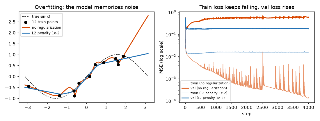
Experiment (the overfit section of ch04_basics.py): a network with about 66,000 parameters (\(1 \to 256 \to 256 \to 1\), ReLU) is trained with Adam (lr 1e-3) for 4000 steps on 12 points with noise of standard deviation 0.3. The L2 penalty multiplies the sum of squares of the parameters whose names contain weight by \(\lambda\) and adds it to the MSE.
| Setting | Final train | Final val | Best val |
| No regularization | 0.0001 | 0.5977 | 0.1709 (step 33) |
| L2 penalty \(\lambda = 10^{-2}\) | 0.0155 | 0.1793 | 0.1709 (step 35) |
Without regularization, the network memorizes even the noise, so the curve wiggles and shoots off wildly at the right end, where there are no points. The validation loss is lowest in the first few dozen steps and then rises again. With L2 regularization, the training loss is slightly higher but the validation loss is much lower.
L2 regularization (weight decay)
An overfitted model's output swings sharply with small changes in the input, and that requires large weights. So a penalty on the size of the weights is added to the loss.
\(L_{\text{total}}(\theta) = L(\theta) + \lambda \sum_{w} w^2\)
\(w \leftarrow w - \eta\Big(\frac{\partial L}{\partial w} + 2\lambda w\Big) = (1 - 2\eta\lambda)\, w - \eta\,\frac{\partial L}{\partial w}\)
Because each step shrinks \(w\) by a factor of \((1 - 2\eta\lambda)\), this is also called weight decay. Weights that the data does not strongly call for are pulled toward 0.
Other remedies:
- Early stopping: use the parameters from the point where the validation loss was lowest. In the experiment above, that is around step 30.
- More data: the most reliable remedy. A world model can keep collecting data by interacting with the environment (Chapter 7).
- Dropout, smaller models, and so on. With Adam,
AdamW, which puts the decay directly into the update rule instead of using an L2 penalty, is common.
Input standardization
When input components differ greatly in scale (an angle from \(-\pi\) to \(\pi\), a velocity from \(-8\) to \(8\)), training slows down. Standardization subtracts the mean from each component and divides by its standard deviation. The world model in Chapter 6 also standardizes both its inputs and outputs.
\(x' = \frac{x - \mu}{s}, \qquad \mu = \frac{1}{N}\sum_i x_i,\quad s = \sqrt{\frac{1}{N}\sum_i (x_i - \mu)^2}\)
Standardized values have mean 0 and variance 1 (\(\frac{1}{N}\sum_i x_i' = \frac{1}{s}(\mu - \mu) = 0\), \(\frac{1}{N}\sum_i x_i'^2 = \frac{s^2}{s^2} = 1\)).
The earlier linear regression shows the effect. Standardizing \(x = (1, 2, 3)\) gives \(\mu = 2\), \(s \approx 0.8165\), and \(x' \approx (-1.2247,\ 0,\ 1.2247)\). The Hessian becomes \(\frac{\partial^2 L}{\partial w^2} = 2\), \(\frac{\partial^2 L}{\partial w\,\partial b} = 0\), \(\frac{\partial^2 L}{\partial b^2} = 2\), so the curvature is 2 in both directions (before standardization it was 11.09 and 0.24, a 46-fold difference). Then \(\eta = 1/2 = 0.5\) reaches the minimum in one step. What standardization does is even out the curvature.
PyTorch tensors and shapes
A tensor is an array of numbers laid out along several axes. A single number is 0-dimensional, a vector is 1-dimensional, a matrix is 2-dimensional, and a batch of images is 4-dimensional. The most important property is the shape, the length along each axis. Most errors in deep learning code are shape mismatches, so the tutorial code records shapes in comments like # (B, T, C).
The results below use a as the (2, 3) tensor [[1, 2, 3], [4, 5, 6]], b as the (3,) tensor [10, 20, 30], c as the (2, 1) tensor [[100], [200]], W with shape (4, 3), and x with shape (5, 3) (the tensors section).
| Expression | Result |
| | 6.0 (indices start at 0) |
| | [5.0, 7.0, 9.0], shape (3,) |
| | [2.0, 5.0], shape (2,) |
| | [[11, 22, 33], [14, 25, 36]] |
| | [[101, 102, 103], [204, 205, 206]] |
| | (5, 4) |
| | (15,) |
| | (1, 5, 3) |
-
dim: selects the axis to reduce along.sum(dim=0)sums along axis 0, which removes that axis, so (2, 3) → (3,). - Broadcasting: when operating on tensors of different shapes, PyTorch aligns the axes starting from the right. If the lengths match, or one of them is 1 (or missing), that axis is copied to fit. (2, 3) + (3,) treats (3,) as (1, 3) and expands it to 2 rows. (2, 3) + (2, 1) expands (2, 1) to 3 columns. (2, 3) + (2,) is an error, because the rightmost axes, 3 and 2, differ.
- Matrix multiplication
@: (5, 3) @ (3, 4) → (5, 4). The inner lengths must match, and that axis disappears.nn.Linear(3, 4)does exactly this and then adds a bias. - Convention: the first axis is the batch. Vector data is (B, D), images are (B, C, H, W) = (batch, channels, height, width), and sequences are (B, T, D) (from Chapter 9).
nn.Module and the five-step training loop
A neural network is written as a class that inherits from nn.Module. __init__ creates the layers and forward defines the forward pass. Autograd handles backpropagation.
class MLP(nn.Module):
    """입력 1개 → 은닉 64 → 은닉 64 → 출력 1개. 은닉층 활성 함수는 tanh."""

    def __init__(self, in_dim=1, hidden=64, out_dim=1, act=nn.Tanh):
        super().__init__()
        self.net = nn.Sequential(
            nn.Linear(in_dim, hidden), act(),
            nn.Linear(hidden, hidden), act(),
            nn.Linear(hidden, out_dim),
        )

    def forward(self, x):  # x: (N, in_dim)
        return self.net(x)  # (N, out_dim)
nn.Linear(n, m) has \(m \times n\) weights and \(m\) biases. This MLP (multi-layer perceptron) has \((1 \times 64 + 64) + (64 \times 64 + 64) + (64 \times 1 + 1) = 128 + 4160 + 65 = 4353\) parameters.
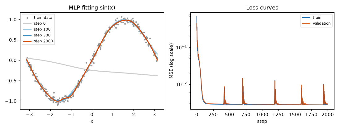
The data is 256 values of \(x\) drawn uniformly from \([-\pi, \pi]\), labeled with \(\sin x + 0.05 \cdot \text{잡음}\), plus a separate validation set of 256 points made the same way (the mlp_data section). The training loop is as follows.
model = MLP().to(device)
optimizer = torch.optim.Adam(model.parameters(), lr=1e-2)
loss_fn = nn.MSELoss()

train_curve, val_curve = [], []
for step in range(steps + 1):
    # (기록) 지금 모델로 그린 곡선을 몇 번 저장해 둔다
    if step in snapshots:
        with torch.no_grad():
            snapshots[step] = model(xs).cpu().numpy()
    if step == steps:
        break
    optimizer.zero_grad()              # ① 지난 스텝의 기울기를 지운다
    y_hat = model(x_train)             # ② 순전파: 예측
    loss = loss_fn(y_hat, y_train)     # ③ 손실 계산
    loss.backward()                    # ④ 역전파: 모든 매개변수의 기울기
    optimizer.step()                   # ⑤ 매개변수 갱신
    with torch.no_grad():              # 검증 손실: 기울기는 필요 없다
        val_loss = loss_fn(model(x_val), y_val)
    train_curve.append(loss.item())
    val_curve.append(val_loss.item())
    if step % 500 == 0 or step == steps - 1:
        print(f"  step {step:4d}  train {loss.item():.5f}  val {val_loss.item():.5f}")
-
optimizer.zero_grad(): every call to.backward()adds the gradient to.grad(it does not overwrite it). Without clearing, gradients accumulate and the parameters move in the wrong direction. - Forward pass
model(x_train): computes the prediction and records the computation graph and intermediate values that backpropagation needs. - Loss:
nn.MSELoss()is the MSE described above. -
loss.backward(): backpropagation. Fills in.gradfor every parameter. -
optimizer.step(): updates the parameters with the Adam update rule.
The validation loss is computed inside torch.no_grad(). No computation graph is recorded, which is faster and saves memory. .item() extracts a single-element tensor as a Python number.
  step    0  train 0.67709  val 0.33090
  step  500  train 0.00282  val 0.00288
  step 1000  train 0.00277  val 0.00285
  step 1500  train 0.00274  val 0.00284
  step 1999  train 0.00273  val 0.00286
  매개변수 개수: 4353
The loss levels off at about 0.0027. The noise added to the data has variance \(0.05^2 = 0.0025\), so going any lower would mean memorizing the noise. Training and validation losses move together, so there is no overfitting. The loss curve has brief spikes up to around \(10^{-2}\) because the learning rate of \(10^{-2}\) is on the high side, and Adam occasionally takes an overly large step. Switching the activation function to nn.ReLU makes the fitted curve look like a chain of straight line segments.
Convolutional neural networks
From Chapter 8 on, the world model sees 64×64 images. Flattening an image into 4096 numbers and feeding it to a linear layer would take \(4096 \times 128 + 128 = 524{,}416\) parameters for a single layer with 128 hidden units, and a bar in the top-left corner and a bar in the bottom-right corner would have to be learned separately. A convolutional neural network (CNN) solves this with two ideas.
- Locality: look at only a small region (for example, 3×3 pixels) at a time. Patterns such as lines and edges live in small regions.
- Weight sharing: slide the same small filter (kernel) across the whole image. The same pattern is detected the same way wherever it appears.
A convolution example
Apply a 3×3 kernel that detects vertical edges to a 4×4 input. Place the kernel over the input, multiply overlapping cells, and sum everything to get one output cell.
\(X = \begin{pmatrix} 1 & 2 & 0 & 1 \\ 0 & 1 & 3 & 1 \\ 2 & 1 & 0 & 0 \\ 1 & 0 & 1 & 2 \end{pmatrix},\qquad K = \begin{pmatrix} 1 & 0 & -1 \\ 1 & 0 & -1 \\ 1 & 0 & -1 \end{pmatrix}\)
\(\begin{align} Y_{11} &= (1 + 0 - 0) + (0 + 0 - 3) + (2 + 0 - 0) = 0 \\ Y_{12} &= (2 + 0 - 1) + (1 + 0 - 1) + (1 + 0 - 0) = 2 \\ Y_{21} &= (0 + 0 - 3) + (2 + 0 - 0) + (1 + 0 - 1) = -1 \\ Y_{22} &= (1 + 0 - 1) + (1 + 0 - 0) + (0 + 0 - 2) = -1 \end{align}\)
\(Y = \begin{pmatrix} 0 & 2 \\ -1 & -1 \end{pmatrix}\)
Each parenthesized group is one row: the left-column value minus the right-column value. In training, the kernel's 9 numbers are parameters, and the data decides which pattern to look for.
Channels: a grayscale image has 1 channel, a color image has 3. nn.Conv2d(C_in, C_out, K) has \(C_{\text{out}}\) kernels, each of size \(C_{\text{in}} \times K \times K\). It has \(C_{\text{out}} \cdot C_{\text{in}} \cdot K \cdot K + C_{\text{out}}\) parameters, and each output channel becomes a map (feature map) showing where a particular pattern appears. PyTorch's "convolution" does not flip the kernel (strictly speaking, it is cross-correlation). Since the kernel is learned, this makes no difference.
Output size formula
The stride \(S\) is how many cells the kernel moves at a time, and the padding \(P\) is how many rows of zeros are added around the edges of the input. The padded length is \(W + 2P\), and the \(n\)-th starting position of the kernel, \(nS\) (\(n = 0, 1, 2, \dots\)), must satisfy \(nS + K \le W + 2P\), so (see Convolution arithmetic)
\(W_{\text{out}} = \left\lfloor \frac{W - K + 2P}{S} \right\rfloor + 1\)
Transposed convolution
A decoder (the VAE in Chapter 8, the RSSM in Chapter 11) has to redraw an image from a small latent vector, and for this it uses transposed convolution (nn.ConvTranspose2d). Each input value stamps a copy of the kernel, scaled by that value, onto the output, and overlapping positions are summed. A 1D example: input \((1, 2)\), kernel \((1, 2, 1)\), stride 2.
\(\begin{align} 1 \times (1, 2, 1) &\to (1,\ 2,\ 1,\ 0,\ 0) && \text{0번 위치에 도장} \\ 2 \times (1, 2, 1) &\to (0,\ 0,\ 2,\ 4,\ 2) && \text{2번 위치에 도장} \\ \text{합} &= (1,\ 2,\ 3,\ 4,\ 2) && \text{길이 2 → 5} \end{align}\)
The output size is the convolution formula solved in reverse (when the division is exact).
\(W_{\text{big}} = (W_{\text{small}} - 1)S - 2P + K\)
| Layer | Computation | Shape change (actual output) |
| | \(\lfloor 62/2 \rfloor + 1 = 32\) (halved) | (1, 1, 64, 64) → (1, 16, 32, 32) |
| | 64 (size preserved) | (1, 1, 64, 64) → (1, 8, 64, 64) |
| | 60 | (1, 1, 64, 64) → (1, 8, 60, 60) |
| | \((4 - 1)\cdot 2 - 2 + 4 = 8\) (doubled) | (1, 64, 4, 4) → (1, 32, 8, 8) |
The earlier 4×4 example gives \(\lfloor (4-3)/1 \rfloor + 1 = 2\), and the 1D transposed convolution example gives \((2-1)\cdot 2 - 0 + 3 = 5\). A transposed convolution with \(K = 4, S = 2, P = 1\) exactly doubles the size, undoing the encoder's 64 → 32 → 16 → 8 → 4 in reverse.
Exercise: reading the angle from a pendulum image
Train a CNN that looks only at the 64×64 grayscale image from PixelPendulum and predicts the bar's angle as \((\cos\theta, \sin\theta)\). This is a scaled-down version of what the VAE encoder does in Chapter 8.
- Data (the
cnn_datasection): run the pendulum with random actions (uniform on \([-2, 2]\)) and collect (image, \([\cos\theta, \sin\theta]\)) pairs. The ground truth is read fromenv.state()[:2]and used only as the label. Training uses 6000 images from 30 episodes, validation 2000 images from 10 episodes. - Preprocessing: divide the 0–255 integers by 255 to scale them to 0–1, and use
unsqueeze(1)to add a channel axis, turning (N, 64, 64) into (N, 1, 64, 64). - Model: four stride-2 convolutions shrink the image 64 → 32 → 16 → 8 → 4, and then linear layers output 2 numbers.
class AngleCNN(nn.Module):
    """64×64 흑백 그림 → [cos θ, sin θ]. 8장 VAE 인코더의 축소판이다."""

    def __init__(self):
        super().__init__()
        self.features = nn.Sequential(
            nn.Conv2d(1, 16, 4, stride=2, padding=1), nn.ReLU(),   # (B, 16, 32, 32)
            nn.Conv2d(16, 32, 4, stride=2, padding=1), nn.ReLU(),  # (B, 32, 16, 16)
            nn.Conv2d(32, 64, 4, stride=2, padding=1), nn.ReLU(),  # (B, 64, 8, 8)
            nn.Conv2d(64, 64, 4, stride=2, padding=1), nn.ReLU(),  # (B, 64, 4, 4)
        )
        self.head = nn.Sequential(
            nn.Flatten(),                                          # (B, 1024)
            nn.Linear(64 * 4 * 4, 128), nn.ReLU(),
            nn.Linear(128, 2),                                     # (B, 2)
        )

    def forward(self, img):  # img: (B, 1, 64, 64)
        return self.head(self.features(img))
The parameters are \(272 + 8{,}224 + 32{,}832 + 65{,}600\) in the convolutions and \(131{,}200 + 258\) in the linear layers, 238,386 in total. That is less than half of what feeding the image straight into a linear layer (128 hidden units) would take. Training (the cnn_train section) runs for 3000 steps with Adam (lr 1e-3), MSE loss, and a random minibatch of 64 images at each step.
  훈련 그림 6000장, 검증 그림 2000장 (모으는 데 2.9초)
  step    0  train 0.51018  val 0.50112
  step  500  train 0.00002  val 0.00003
  step 1000  train 0.00003  val 0.00004
  step 1500  train 0.00001  val 0.00002
  step 2000  train 0.00005  val 0.00003
  step 2500  train 0.00001  val 0.00001
  step 3000  train 0.00003  val 0.00005
  수집 + 학습 시간 200.7초 (장치: cpu)
  검증 각도 오차: 평균 0.26°, 중앙값 0.21°, 최대 0.66°
- Figure: True and predicted directions over validation images, and a scatter plot of true vs. predicted angle
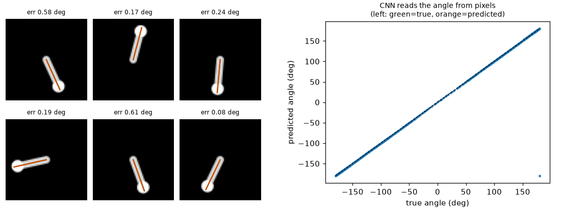
The lone point in the corner of the scatter plot is not an error. It is a plotting artifact at the boundary, because \(+180^\circ\) and \(-180^\circ\) are the same pose. This is also why the angle is predicted as \(\cos\) and \(\sin\) (Chapter 6).
This CNN cannot predict the angular velocity \(\dot\theta\), because a single image contains no information about how fast the pendulum is swinging. This limitation is the partial observability problem from Chapter 5, and Chapters 9 and 11 solve it by adding memory (an RNN).
Summary
- A neural network is a function \(f_\theta\) with parameters \(\theta\), and training means finding a \(\theta\) that reduces the loss \(L(\theta)\).
- A derivative is a slope, and the chain rule says "rates of change multiply". The gradient vector \(\nabla L\) points uphill along the steepest direction.
- Gradient descent \(\theta \leftarrow \theta - \eta\nabla L\) reduces the loss by \(\eta\lVert\nabla L\rVert^2\) to first order. Along a direction with curvature \(a\), convergence requires \(\eta \lt 2/a\).
- Backpropagation is the chain rule applied from the output backward, passing on (received gradient) × (local derivative). Autograd performs the same computation.
- The gradient of softmax plus cross-entropy is \(p - y\). The minibatch gradient is an unbiased estimate, and Adam uses two moments with bias correction \(1/(1-\beta^t)\).
- Overfitting is detected with validation data and prevented with L2 regularization (weight decay), early stopping, and more data. Standardization evens out the curvature.
- The five-step training loop:
zero_grad→ forward pass → loss →backward→step. - A CNN reads images using locality and weight sharing. The output size is \(\lfloor (W - K + 2P)/S \rfloor + 1\), and for a transposed convolution it is \((W-1)S - 2P + K\).
Review questions
- 1. The derivative of \(f(x) = \log(1 + x^2)\) and its value at \(x = 1\)
- By the chain rule, \(f'(x) = \frac{2x}{1 + x^2}\), and \(f'(1) = 1\).
- 2. For \(L(w) = 2w^2\), the range of learning rates for which gradient descent converges, and the learning rate that reaches the minimum in one step
- Since \(a = 4\), \(0 \lt \eta \lt 2/a = 0.5\). With \(\eta = 1/a = 0.25\), it reaches 0 in one step.
- 3. The output shape and parameter count when (1, 3, 32, 32) is fed into
nn.Conv2d(3, 8, kernel_size=3, stride=2, padding=1) - \(\lfloor (32 - 3 + 2)/2 \rfloor + 1 = 16\), so the shape is (1, 8, 16, 16). There are \(8 \times 3 \times 3 \times 3 + 8 = 224\) parameters.
- 4. The cross-entropy loss and gradient for logits \(z = (0, 0)\) with correct class 0
- \(p = (0.5, 0.5)\), \(L = \log 2 \approx 0.693\), \(\partial L/\partial z = p - y = (-0.5,\ 0.5)\).
- 5. In Adam with \(\beta_1 = 0.9\), \(m_2\) and \(\hat{m}_2\) when the gradients of the first two steps are both \(g\)
- \(m_1 = 0.1g\), \(m_2 = 0.9 \times 0.1g + 0.1g = 0.19g\), \(\hat{m}_2 = \frac{0.19g}{1 - 0.9^2} = g\).
- 6. What happens if
optimizer.zero_grad()is left out of the training loop -
.backward()adds gradients to.grad, so the gradient at step \(t\) becomes the sum of all gradients so far. The steps keep growing and point in the wrong direction, so training becomes unstable or diverges.
See also
- World Models:Tutorial
- World Models
- Deep learning
- PyTorch
- Gradient descent
- Stochastic gradient descent
- Backpropagation
- Gradient Vanishing
- Softmax
- Cross entropy
- CNN
- Convolution
- Convolution arithmetic