WorldModels:Tutorial:03-InformationTheory
lastmod 2026-11-18created 2026-11-172 edits
Information theory and KL divergence is chapter 3 of the World Model tutorial. It derives the KL divergence (Kullback–Leibler divergence), which appears in every loss function of VAE (chapter 8), RSSM (chapter 11), and Dreamer (chapter 12), starting from the intuition of "amount of surprise" and moving through information content, entropy, and cross-entropy. It covers why KL is always non-negative (Jensen's inequality), how KL behaves differently depending on its direction, the closed form of KL between two Gaussians, and mutual information, and it previews the derivation of the ELBO in chapter 8.
- Original: 03. Math ② Information Theory and KL Divergence
- Code:
code/ch03_information.py(a few seconds on CPU;--quickreduces the number of samples from 1,000,000 to 10,000) - Previous: 02. Probability and Maximum Likelihood / Next: 04. Deep Learning and PyTorch Basics
Why information theory
Maximum likelihood from chapter 2 is the principle for fitting a model to data. When building a World Model, another situation keeps coming up: "we want to make two distributions close."
| Chapter | What is needed |
| Chapter 8 VAE | Keep the latent distribution \(q_\phi(z \mid o)\) produced by the encoder close to the reference distribution \(p(z) = \mathcal{N}(0, I)\) (a standard normal distribution with independent components). |
| Chapter 11 RSSM | Bring the state distribution inferred from the image (posterior) close to the state distribution predicted by imagination alone, without the image (prior). |
| Chapter 12 Dreamer | Keep the policy's entropy high so that it does not collapse to one side. |
The standard tool for measuring "how different two distributions are" is the KL divergence, and its roots lie in the information theory founded by Claude Shannon in 1948.
Information content
The rarer an event, the more surprising the news that it happened, and the more information that news carries. The surprise when an event of probability \(p\) occurs, i.e. its information content (surprisal) \(I(p)\), is required to satisfy three conditions.
- A certain event is not surprising: \(I(1) = 0\).
- Rarer means more surprising: as \(p\) gets smaller, \(I(p)\) gets larger.
- When two independent events occur together, their surprises add: \(I(p_1 p_2) = I(p_1) + I(p_2)\).
These three conditions alone determine the form of \(I\). Assume \(I\) is differentiable, differentiate condition 3 with respect to \(y\), and then set \(y = 1\).
\(\begin{align} I(xy) &= I(x) + I(y) \qquad (0 \lt x, y \le 1) \\ x\, I'(xy) &= I'(y) \\ x\, I'(x) &= I'(1) =: -c \qquad (c \gt 0,\ \text{condition 2}) \\ I'(x) &= -\frac{c}{x} \;\Rightarrow\; I(x) = -c\log x + C \\ I(p) &= -c\,\log p \qquad (C = 0,\ \text{condition 1}) \end{align}\)
Information content is the negative log probability, and \(c\) only sets the unit. With \(c = 1\) and the natural logarithm the unit is the nat; with the base-2 logarithm it is the bit (\(c = 1/\log 2\)). This tutorial uses the natural logarithm (nats).
| Probability of the event \(p\) | Information content (nats) \(-\log p\) | Information content (bits) \(-\log_2 p\) |
| 1 (certain) | 0 | 0 |
| 1/2 (coin lands heads) | 0.693 | 1 |
| 1/8 | 2.079 | 3 |
| 0.01 | 4.605 | 6.644 |
The NLL \(-\log p_\theta(x)\) from chapter 2 is the surprise the model feels when it sees the data. Maximum likelihood training makes the model less surprised by the real data.
Entropy
Entropy is the expected surprise when outcomes are drawn from a distribution \(p\), and it measures the distribution's uncertainty.
\(H(p) = \mathbb{E}_{x \sim p}[-\log p(x)] = -\sum_x p(x)\log p(x)\)
For outcomes with probability 0, \(0 \cdot \log 0\) is taken to be 0, because \(p\log p \to 0\) as \(p \to 0\) (\(0.1\log 0.1 = -0.230\), \(0.01\log 0.01 = -0.046\), \(0.001\log 0.001 = -0.0069\)).
Entropy of a coin
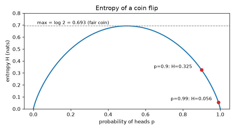
The entropy of a coin with probability \(p\) of heads is:
\(H(p) = -p\log p - (1 - p)\log(1 - p)\)
| Probability of heads | Entropy (nats) | Entropy (bits) |
| 0.5 | \(\log 2 = 0.6931\) | 1.0000 |
| 0.9 | 0.3251 | 0.4690 |
| 0.99 | 0.0560 | 0.0808 |
Differentiation confirms that the maximum is at \(p = 1/2\). Since \(\frac{d}{dp}(p\log p) = \log p + 1\),
\(\begin{align} H'(p) &= -(\log p + 1) + (\log(1-p) + 1) = \log\frac{1 - p}{p} \\ H'(p) &= 0 \;\Leftrightarrow\; p = \tfrac12 \\ H''(p) &= -\frac{1}{p} - \frac{1}{1-p} \lt 0 \end{align}\)
The curve is a concave hill with peak value \(H(\tfrac12) = \log 2\). In general, the entropy of a distribution with \(K\) outcomes is maximized by the uniform distribution, with value \(\log K\) (the proof is in "Why KL is non-negative" below).
Differential entropy of a Gaussian
For continuous distributions, the integral \(H(p) = -\int p(x)\log p(x)\,dx\) replaces the sum, and this is called differential entropy. Plugging in the Gaussian log-density formula from chapter 2 gives
\(\begin{align} H &= \mathbb{E}\left[\frac12\log(2\pi) + \log\sigma + \frac{(x-\mu)^2}{2\sigma^2}\right] \\ &= \frac12\log(2\pi) + \log\sigma + \frac{\mathbb{E}[(x - \mu)^2]}{2\sigma^2} = \frac12\log(2\pi) + \log\sigma + \frac12 \\ H\big(\mathcal{N}(\mu, \sigma^2)\big) &= \frac12\log(2\pi e\,\sigma^2) \end{align}\)
- It does not depend on the mean \(\mu\) and grows with the spread \(\sigma\).
- With \(\sigma = 1\) it is 1.419 nats; with \(\sigma = 0.1\) it is \(1.419 + \log 0.1 = -0.884\) nats. Because a density can exceed 1, differential entropy can be negative.
- The entropy of the action distribution in Dreamer (chapter 12) starts from this formula (there, one more correction term is added to account for squashing actions with \(\tanh\)).
Cross-entropy
If outcomes actually come from a distribution \(p\) but you believe they come from \(q\), the surprise felt for each outcome is \(-\log q(x)\), and its average is taken over the real distribution \(p\). This is cross-entropy.
\(H(p, q) = \mathbb{E}_{x \sim p}[-\log q(x)] = -\sum_x p(x)\log q(x)\)
An example with true distribution \(p = (0.5, 0.3, 0.2)\) and model \(q = (0.4, 0.4, 0.2)\):
\(\begin{align} H(p) &= -(0.5\log 0.5 + 0.3\log 0.3 + 0.2\log 0.2) = 0.3466 + 0.3612 + 0.3219 = 1.0297 \\ H(p, q) &= -(0.5\log 0.4 + 0.3\log 0.4 + 0.2\log 0.2) = 0.4581 + 0.2749 + 0.3219 = 1.0549 \end{align}\)
The model's probabilities \(q\) go inside the logarithm, and the true probabilities \(p\) serve as the weights. The wrong belief raised the average surprise from 1.0297 to 1.0549.
This is the classification loss "cross-entropy" from chapter 2. A label of class \(y\) means \(p\) is a one-hot distribution that puts 1 on \(y\) only, and then \(H(p, q) = -\log q(y)\), which is the categorical NLL.
KL divergence
The extra surprise caused by the wrong belief \(q\), i.e. cross-entropy minus entropy, is the KL divergence. Kullback and Leibler defined it in 1951.
\(\begin{align} H(p, q) - H(p) &= -\sum_x p(x)\log q(x) + \sum_x p(x)\log p(x) \\ D_{\mathrm{KL}}(p \,\|\, q) &= \sum_x p(x)\log\frac{p(x)}{q(x)} = \mathbb{E}_{x \sim p}\!\left[\log\frac{p(x)}{q(x)}\right] \end{align}\)
For continuous distributions the sum becomes an integral. For the example above:
- \(D_{\mathrm{KL}}(p \,\|\, q) = 1.05492 - 1.02965 = 0.0253\). Computing it from the definition, \(0.5\log\frac{0.5}{0.4} + 0.3\log\frac{0.3}{0.4} + 0.2\log\frac{0.2}{0.2} = 0.1116 - 0.0863 + 0 = 0.0253\), gives the same result.
- Swapping the order gives a different value: \(D_{\mathrm{KL}}(q \,\|\, p) = 0.4\log\frac{0.4}{0.5} + 0.4\log\frac{0.4}{0.3} + 0 = -0.0893 + 0.1151 = 0.0258\).
def entropy(p: np.ndarray) -> float:
    """H(p) = -Σ p_i log p_i   (p_i = 0 인 항은 0 으로 친다: 0·log 0 = 0)"""
    p = p[p > 0]
    return float(-np.sum(p * np.log(p)))


def cross_entropy(p: np.ndarray, q: np.ndarray) -> float:
    """H(p, q) = -Σ p_i log q_i   (정답 분포 p 로 평균 낸, 모델 q 의 놀람)"""
    mask = p > 0
    return float(-np.sum(p[mask] * np.log(q[mask])))


def kl(p: np.ndarray, q: np.ndarray) -> float:
    """KL(p ‖ q) = Σ p_i log(p_i / q_i)"""
    mask = p > 0
    return float(np.sum(p[mask] * np.log(p[mask] / q[mask])))
mask = p > 0 implements the convention of dropping terms where \(p(x) = 0\), treating \(0 \cdot \log(0/q)\) as 0. The output of discrete_examples() in the same region (discrete) is:
[엔트로피] 앞면 확률  0.5: H = 0.6931 nats = 1.0000 bits
[엔트로피] 앞면 확률  0.9: H = 0.3251 nats = 0.4690 bits
[엔트로피] 앞면 확률 0.99: H = 0.0560 nats = 0.0808 bits
[이산] H(p) = 1.0297,  H(p,q) = 1.0549
[이산] KL(p‖q) = 0.0253,  H(p,q) - H(p) = 0.0253
[이산] KL(q‖p) = 0.0258   ← 순서를 바꾸면 값이 다르다 (비대칭)
[이산] 균등 분포 3칸의 엔트로피 = 1.0986 = log 3 = 1.0986
Properties of KL
- Always non-negative: \(D_{\mathrm{KL}}(p \,\|\, q) \ge 0\), and it is 0 only when the distributions are identical.
- Asymmetric: in general \(D_{\mathrm{KL}}(p \,\|\, q) \ne D_{\mathrm{KL}}(q \,\|\, p)\). That is why it is called a divergence rather than a distance.
- Infinite if \(p\) has mass where \(q\) is 0: if \(p(x) \gt 0\) and \(q(x) = 0\), then \(\log(p/0) = \infty\). It is the price of believing that something possible is impossible.
Maximum likelihood is KL minimization
Let \(p_{\text{data}}\) be the true distribution that generated the data and \(p_\theta\) the model.
\(\begin{align} D_{\mathrm{KL}}(p_{\text{data}} \,\|\, p_\theta) &= \mathbb{E}_{x \sim p_{\text{data}}}[\log p_{\text{data}}(x)] - \mathbb{E}_{x \sim p_{\text{data}}}[\log p_\theta(x)] \\ &= -H(p_{\text{data}}) - \mathbb{E}_{x \sim p_{\text{data}}}[\log p_\theta(x)] \\ \operatorname*{arg\,min}_\theta D_{\mathrm{KL}}(p_{\text{data}} \,\|\, p_\theta) &= \operatorname*{arg\,max}_\theta \mathbb{E}_{x \sim p_{\text{data}}}[\log p_\theta(x)] \approx \operatorname*{arg\,max}_\theta \frac{1}{N}\sum_{i=1}^N \log p_\theta(x_i) \end{align}\)
The first term, \(-H(p_{\text{data}})\), is a constant independent of \(\theta\). The expectation over the true distribution is unknown, so estimating it by Monte Carlo as the average over \(N\) data points gives the average log-likelihood, i.e. maximum likelihood. Maximum likelihood training pulls the model distribution toward the data distribution so that the KL shrinks, and the direction is \(D_{\mathrm{KL}}(p_{\text{data}} \,\|\, p_\theta)\), with the data first.
Convex functions and Jensen's inequality
Proving that KL is non-negative and deriving the ELBO in chapter 8 both require Jensen's inequality.
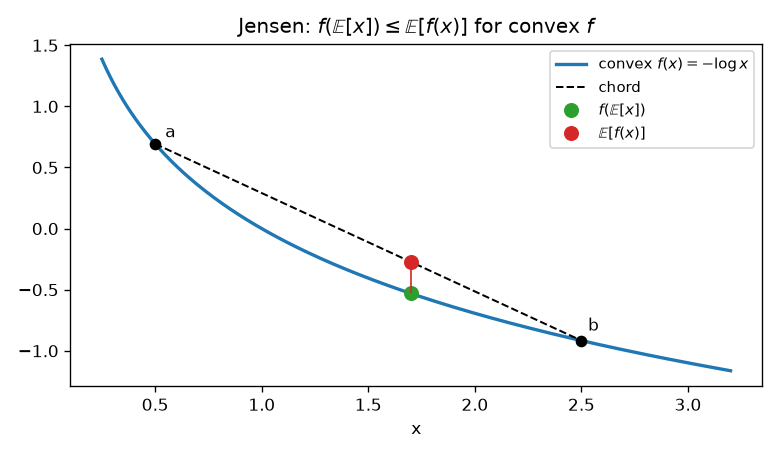
A function \(f\) is convex if the line segment (chord) joining any two points on its graph always lies above the graph. For two points \(a, b\) and a mixing weight \(w \in [0, 1]\),
\(f\big(w\,a + (1 - w)\,b\big) \;\le\; w\,f(a) + (1 - w)\,f(b)\)
The left side is the function value at the mixed point (a point on the curve); the right side is the mix of function values (a point on the chord). If the chord always lies below the graph, the function is concave and the inequality flips. A twice-differentiable function is convex if \(f''(x) \ge 0\) and concave if \(f''(x) \le 0\).
| Function | Second derivative | Verdict |
| \(x^2\) | \(2 \ge 0\) | Convex |
| \(-\log x\) (\(x \gt 0\)) | \(1/x^2 \gt 0\) | Convex |
| \(\log x\) | \(-1/x^2 \lt 0\) | Concave |
| \(e^x\) | \(e^x \gt 0\) | Convex |
Extending the two-point definition to many points gives Jensen's inequality. For three points with weights \(w_i \ge 0\), \(w_1 + w_2 + w_3 = 1\) (and \(w_1 \lt 1\)), group the last two terms into a single point \(m\) and apply the two-point definition twice.
\(\begin{align} w_1 x_1 + w_2 x_2 + w_3 x_3 &= w_1 x_1 + (1 - w_1)\,m, \qquad m := \frac{w_2 x_2 + w_3 x_3}{1 - w_1} \\ f(w_1 x_1 + (1-w_1)\,m) &\le w_1 f(x_1) + (1 - w_1)\,f(m) \\ f(m) &\le \frac{w_2}{1 - w_1}f(x_2) + \frac{w_3}{1 - w_1}f(x_3) \\ f(w_1 x_1 + w_2 x_2 + w_3 x_3) &\le w_1 f(x_1) + w_2 f(x_2) + w_3 f(x_3) \end{align}\)
Repeating the same argument (mathematical induction) shows it holds for any number of points. Treating the weights \(w_i\) as probabilities \(p(x_i)\), it can be written as follows, and the same holds for continuous distributions.
\(\text{convex } f: \quad f(\mathbb{E}[X]) \le \mathbb{E}[f(X)], \qquad\qquad \text{concave } f: \quad f(\mathbb{E}[X]) \ge \mathbb{E}[f(X)]\)
In particular, \(\log\) is concave, so the following holds. It is the inequality used most in this chapter and chapter 8.
\(\log \mathbb{E}[X] \;\ge\; \mathbb{E}[\log X]\)
def jensen_check(rng: np.random.Generator, n: int) -> None:
    """log 는 오목(위로 볼록) 함수라서 log E[X] ≥ E[log X] 이다."""
    x = rng.uniform(0.5, 2.0, size=n)  # 양수인 확률변수
    print(f"[젠센] log E[X] = {math.log(x.mean()):.4f}  ≥  E[log X] = {np.log(x).mean():.4f}")
    x2 = rng.normal(0.0, 1.0, size=n)
    print(f"[젠센] (E[X])² = {x2.mean() ** 2:.4f}  ≤  E[X²] = {(x2**2).mean():.4f}   (x² 는 볼록)")
- By hand: if \(X\) is uniform between 0.5 and 2, then \(\mathbb{E}[X] = 1.25\), \(\log 1.25 = 0.2231\), and \(\mathbb{E}[\log X] = \frac{1}{1.5}\big[x\log x - x\big]_{0.5}^{2} = \frac{(1.3863 - 2) - (-0.3466 - 0.5)}{1.5} = 0.1553\).
- The second line says the same thing as chapter 2's "variance ≥ 0, i.e. \(\mathbb{E}[X^2] \ge (\mathbb{E}[X])^2\)" (\(x^2\) is convex).
- Figure: Figure 3-2. For the convex function -log x, mixing the points a = 0.5 and b = 2.5 in a 4:6 ratio puts the function value at the mean below the average of the function values on the chord
Why KL is non-negative
Proof 1: Jensen's inequality
The sum runs only over \(x\) with \(p(x) \gt 0\).
\(\begin{align} -D_{\mathrm{KL}}(p \,\|\, q) &= \sum_{x:\,p(x) \gt 0} p(x)\log\frac{q(x)}{p(x)} = \mathbb{E}_{x \sim p}\!\left[\log\frac{q(x)}{p(x)}\right] \\ &\le \log \mathbb{E}_{x \sim p}\!\left[\frac{q(x)}{p(x)}\right] = \log\sum_{x:\,p(x) \gt 0} q(x) \\ &\le \log 1 = 0 \end{align}\)
The second line follows from the concavity of \(\log\) (\(\mathbb{E}[\log Y] \le \log\mathbb{E}[Y]\) with \(Y = q(x)/p(x)\)), and the third from the fact that a sum over only some of \(q\)'s entries is at most 1.
Proof 2: log t ≤ t − 1
\(g(t) = t - 1 - \log t\) is convex since \(g''(t) = 1/t^2 \gt 0\), and \(g'(1) = 0\), \(g(1) = 0\), so it has a minimum of 0 at \(t = 1\). Hence \(\log t \le t - 1\), with equality only at \(t = 1\). Substitute \(t = q(x)/p(x)\) into each term.
\(\begin{align} -D_{\mathrm{KL}}(p \,\|\, q) &= \sum_{p \gt 0} p(x)\log\frac{q(x)}{p(x)} \le \sum_{p \gt 0} p(x)\left(\frac{q(x)}{p(x)} - 1\right) \\ &= \sum_{p \gt 0} q(x) - \sum_{p \gt 0} p(x) \le 1 - 1 = 0 \end{align}\)
Equality holds only when \(q(x)/p(x) = 1\) everywhere, i.e. \(p = q\).
Consequences
- Cross-entropy ≥ entropy (Gibbs' inequality): \(H(p, q) = H(p) + D_{\mathrm{KL}}(p \,\|\, q) \ge H(p)\). For data where the same input can have several correct answers, the average classification loss cannot go down to 0; the entropy of the label distribution is the floor. With one-hot labels, where the answer is always unique, \(H(p) = 0\) and the floor is 0 too.
- Entropy ≤ log K: the KL to the uniform distribution \(u(x) = 1/K\) is \(D_{\mathrm{KL}}(p \,\|\, u) = \sum_x p\log p + \log K\sum_x p = -H(p) + \log K \ge 0\). Hence \(H(p) \le \log K\), with equality when \(p = u\) (\(\log 3 = 1.0986\) for 3 outcomes).
Direction of KL: forward and reverse
When \(p\) is the distribution to be matched and \(q\) is the adjustable model, there are two directions.
| Direction | Formula | Behavior | Where it is used |
| forward KL | \(D_{\mathrm{KL}}(p \Vert q) = \mathbb{E}_{x\sim p}[\log p(x) - \log q(x)]\) | Averaged over \(p\). If \(q\) is small where \(p\) has mass, \(-\log q\) blows up, so \(q\) spreads out widely to cover everywhere \(p\) has mass (mode covering). | Maximum likelihood in chapter 2 |
| reverse KL | \(D_{\mathrm{KL}}(q \Vert p) = \mathbb{E}_{x\sim q}[\log q(x) - \log p(x)]\) | Averaged over \(q\). It is penalized if \(p\) is small where \(q\) has mass, so \(q\) avoids regions where \(p\) is nearly zero and sticks to a single peak (mode seeking). | Variational inference in chapter 8 (training the VAE encoder) |
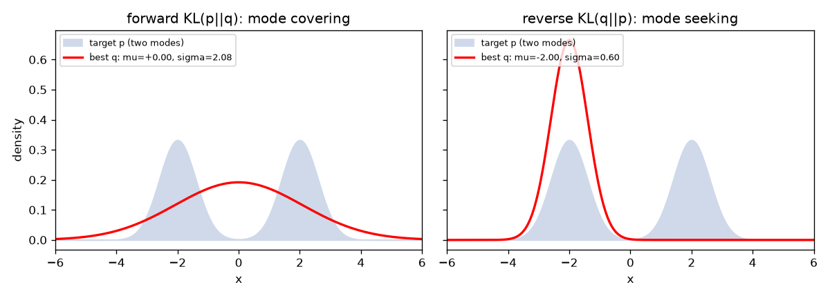
This is checked with an experiment that fits a single Gaussian \(q = \mathcal{N}(\mu, \sigma^2)\) to a two-peaked distribution \(p(x) = \frac12\mathcal{N}(x; -2, 0.6^2) + \frac12\mathcal{N}(x; 2, 0.6^2)\).
Forward KL solution: moment matching
\(\begin{align} D_{\mathrm{KL}}(p \,\|\, q) &= \underbrace{\mathbb{E}_p[\log p(x)]}_{\text{independent of } q} + \mathbb{E}_p\!\left[\frac12\log(2\pi) + \log\sigma + \frac{(x - \mu)^2}{2\sigma^2}\right] \\ \frac{\partial}{\partial\mu}: &\; -\frac{\mathbb{E}_p[x - \mu]}{\sigma^2} = 0 \;\Rightarrow\; \mu^\ast = \mathbb{E}_p[x] \\ \frac{\partial}{\partial\sigma}: &\; \frac{1}{\sigma} - \frac{\mathbb{E}_p[(x - \mu)^2]}{\sigma^3} = 0 \;\Rightarrow\; \sigma^{\ast 2} = \operatorname{Var}_p[x] \end{align}\)
This is the same calculation as the Gaussian MLE in chapter 2, and matching the mean and variance directly is called moment matching. For the mixture, \(\mathbb{E}_p[x] = 0\) and \(\mathbb{E}_p[x^2] = 0.6^2 + 2^2 = 4.36\), so \(\mu^\ast = 0\) and \(\sigma^\ast = \sqrt{4.36} \approx 2.09\). The result is a Gaussian centered at \(x = 0\), where there is almost no actual mass, spread widely to cover both peaks.
Estimating the size of the reverse KL
The reverse KL has no closed-form solution, so it is found by grid search. Suppose \(q\) equals the left component \(g_1 = \mathcal{N}(-2, 0.6^2)\). Then \(x \approx -2\) is about 6.7 standard deviations from the center of the right peak, so \(g_2(x) \approx 0\) and \(p(x) \approx \tfrac12 q(x)\).
\(D_{\mathrm{KL}}(q \,\|\, p) = \mathbb{E}_q\!\left[\log\frac{q(x)}{p(x)}\right] \approx \mathbb{E}_q\!\left[\log\frac{q(x)}{\frac12 q(x)}\right] = \log 2 \approx 0.693\)
Ignoring the right peak entirely costs only \(\log 2\). Spreading out between the two would put mass in the valley where \(p \approx 0\) and incur a larger penalty.
Grid search experiment
def forward_reverse_kl(fig_dir: str) -> None:
    """봉우리가 두 개인 p 에 가우시안 q 하나를 맞춘다. KL 의 방향에 따라 결과가 다르다."""
    xs = np.linspace(-8, 8, 4001)
    dx = xs[1] - xs[0]

    def normal_pdf(x, mu, s):
        return np.exp(-((x - mu) ** 2) / (2 * s**2)) / (s * math.sqrt(2 * math.pi))

    p = 0.5 * normal_pdf(xs, -2, 0.6) + 0.5 * normal_pdf(xs, 2, 0.6)
    eps = 1e-300  # log 0 을 피하는 아주 작은 수

    def kl_num(a, b):  # 격자 위에서 적분: Σ a(x) log(a(x)/b(x)) Δx
        return float(np.sum(a * (np.log(a + eps) - np.log(b + eps))) * dx)

    best_fwd, best_rev = (None, math.inf), (None, math.inf)
    for mu in np.linspace(-3, 3, 121):
        for s in np.linspace(0.2, 3.0, 141):
            q = normal_pdf(xs, mu, s)
            f, r = kl_num(p, q), kl_num(q, p)
            if f < best_fwd[1]:
                best_fwd = ((mu, s), f)
            if r < best_rev[1]:
                best_rev = ((mu, s), r)
(The rest, which prints the output and draws the figure, is in region fwd_rev of ch03_information.py.)
[forward KL(p‖q) 최소] μ = +0.00, σ = 2.08  (KL = 0.555)
[reverse KL(q‖p) 최소] μ = -2.00, σ = 0.60  (KL = 0.692)
[참고] p 의 평균 = 0, 분산 = 0.6² + 2² = 4.36 → 표준편차 2.09
- The grid search results (σ = 2.08 for forward, KL = 0.692 for reverse) agree with the hand calculations (2.09 and log 2 = 0.693, respectively).
- Because \(p\) is symmetric, the right peak (\(\mu = +2\)) is an equally good answer for the reverse KL.
- Figure: Figure 3-3. Left: a wide, centered Gaussian fitted with forward KL. Right: a Gaussian on one peak fitted with reverse KL
What this means for World Models:
- A World Model trained with MSE (Gaussian maximum likelihood) predicts a blurry average at a fork (the multimodality problem from chapter 1) because of the "covering" property of forward KL.
- The VAE encoder is trained with reverse KL and tends to produce a distribution narrower (more overconfident) than the true posterior.
- Neither direction is better or worse; they simply behave differently.
The interactive demo in the original (computing the KL between two Gaussians in both directions) shows the same thing. Making \(q\) narrow and placing it in the middle of \(p\) makes \(D_{\mathrm{KL}}(q \,\|\, p)\) small but \(D_{\mathrm{KL}}(p \,\|\, q)\) large (\(q\) cannot cover \(p\)'s tails). Making \(q\) wide does the opposite. The two values are equal only in special cases, such as when the distributions are identical (both 0) or when the two standard deviations are equal (if \(\sigma_p = \sigma_q = \sigma\), both are \((\mu_p - \mu_q)^2/(2\sigma^2)\)).
KL between Gaussians
VAE, RSSM, and Dreamer compute the KL between two Gaussians at every training step. This value has a closed form computed from the means and standard deviations alone, with no integral. Let \(q = \mathcal{N}(\mu_1, \sigma_1^2)\) and \(p = \mathcal{N}(\mu_2, \sigma_2^2)\), and compute \(D_{\mathrm{KL}}(q \,\|\, p)\).
Deriving the closed form
\(\begin{align} D_{\mathrm{KL}}(q \,\|\, p) &= \mathbb{E}_{x \sim q}\big[\log q(x) - \log p(x)\big] \\ \log q(x) - \log p(x) &= \log\frac{\sigma_2}{\sigma_1} - \frac{(x - \mu_1)^2}{2\sigma_1^2} + \frac{(x - \mu_2)^2}{2\sigma_2^2} \\ D_{\mathrm{KL}} &= \log\frac{\sigma_2}{\sigma_1} - \frac{\mathbb{E}_q[(x - \mu_1)^2]}{2\sigma_1^2} + \frac{\mathbb{E}_q[(x - \mu_2)^2]}{2\sigma_2^2} \end{align}\)
The \(-\tfrac12\log(2\pi)\) terms of the two log-densities cancel. Of the two remaining expectations, the first is \(\sigma_1^2\) by the definition of \(q\)'s variance. The second is expanded by subtracting and adding \(\mu_1\).
\(\begin{align} (x - \mu_2)^2 &= (x-\mu_1)^2 + 2(x - \mu_1)(\mu_1 - \mu_2) + (\mu_1 - \mu_2)^2 \\ \mathbb{E}_q[(x - \mu_2)^2] &= \sigma_1^2 + 2(\mu_1 - \mu_2)\underbrace{\mathbb{E}_q[x - \mu_1]}_{=\,0} + (\mu_1 - \mu_2)^2 = \sigma_1^2 + (\mu_1 - \mu_2)^2 \end{align}\)
Substituting, the middle term becomes \(\sigma_1^2/(2\sigma_1^2) = 1/2\), giving the closed form.
\(D_{\mathrm{KL}}\big(\mathcal{N}(\mu_1, \sigma_1^2) \,\|\, \mathcal{N}(\mu_2, \sigma_2^2)\big) = \log\frac{\sigma_2}{\sigma_1} + \frac{\sigma_1^2 + (\mu_1 - \mu_2)^2}{2\sigma_2^2} - \frac12\)
Checks:
- Identical distributions (\(\mu_1 = \mu_2\), \(\sigma_1 = \sigma_2\)): \(\log 1 + \frac{\sigma^2 + 0}{2\sigma^2} - \frac12 = 0\).
- \(q = \mathcal{N}(1, 0.5^2)\), \(p = \mathcal{N}(0, 1)\): \(\log\frac{1}{0.5} + \frac{0.25 + 1}{2} - \frac12 = 0.6931 + 0.625 - 0.5 = 0.8181\).
- Reversed order \(D_{\mathrm{KL}}(p \,\|\, q)\) (\(\mu_1 = 0, \sigma_1 = 1, \mu_2 = 1, \sigma_2 = 0.5\)): \(\log\frac{0.5}{1} + \frac{1 + 1}{2 \times 0.25} - \frac12 = -0.6931 + 4 - 0.5 = 2.8069\). The asymmetry is large.
- With equal variances it reduces to \((\mu_1 - \mu_2)^2/(2\sigma^2)\).
KL to the standard normal (the special case used by VAE)
Chapter 8 only uses the case where the reference distribution is the standard normal \(p = \mathcal{N}(0, 1)\). Plugging in \(\mu_2 = 0\), \(\sigma_2 = 1\) and using \(\log\frac{1}{\sigma} = -\frac12\log\sigma^2\) gives
\(D_{\mathrm{KL}}\big(\mathcal{N}(\mu, \sigma^2) \,\|\, \mathcal{N}(0, 1)\big) = \frac12\big(\mu^2 + \sigma^2 - 1 - \log\sigma^2\big)\)
It is 0 only when \(\mu = 0\) and \(\sigma = 1\), and it grows as the mean moves away from 0 or the standard deviation moves away from 1. With \(\mu = 1\), \(\sigma = 0.5\), \(\frac12(1 + 0.25 - 1 - \log 0.25) = \frac12(0.25 + 1.3863) = 0.8181\), the same value as the general formula.
Diagonal Gaussian: sum of per-dimension KLs
Latent variables usually have dozens of dimensions and are diagonal Gaussians with independent dimensions. The density is the product of per-dimension densities, so the log is the sum of per-dimension logs, and each term depends only on \(x_d\).
\(\begin{align} D_{\mathrm{KL}}(q \,\|\, p) &= \sum_{d=1}^D \mathbb{E}_{x \sim q}\big[\log q_d(x_d) - \log p_d(x_d)\big] \\ &= \sum_{d=1}^D \mathbb{E}_{x_d \sim q_d}\big[\log q_d(x_d) - \log p_d(x_d)\big] = \sum_{d=1}^D D_{\mathrm{KL}}(q_d \,\|\, p_d) \end{align}\)
Example: with \(\mu = (1, -0.5, 0)\) and \(\sigma = (0.5, 1, 2)\), the per-dimension values are 0.8181, \(\frac12(0.25 + 1 - 1 - 0) = 0.125\), and \(\frac12(0 + 4 - 1 - \log 4) = 0.8069\), summing to 1.75.
Comparing the closed form, Monte Carlo, and PyTorch
def kl_gauss(mu1: float, s1: float, mu2: float, s2: float) -> float:
    """KL( N(μ1, s1²) ‖ N(μ2, s2²) ) 닫힌 꼴 = log(s2/s1) + (s1² + (μ1-μ2)²) / (2 s2²) - 1/2"""
    return math.log(s2 / s1) + (s1**2 + (mu1 - mu2) ** 2) / (2 * s2**2) - 0.5


def kl_to_standard_normal(mu: float, s: float) -> float:
    """VAE 에서 쓰는 특수형: KL( N(μ, s²) ‖ N(0, 1) ) = ½ (μ² + s² - 1 - log s²)"""
    return 0.5 * (mu**2 + s**2 - 1 - math.log(s**2))


def gaussian_kl_check(rng: np.random.Generator, n: int, fig_dir: str) -> None:
    mu1, s1, mu2, s2 = 1.0, 0.5, 0.0, 1.0
    closed = kl_gauss(mu1, s1, mu2, s2)

    # 몬테카를로: x ~ q 를 많이 뽑아 log q(x) - log p(x) 를 평균 낸다.
    def log_normal(x, mu, s):
        return -0.5 * math.log(2 * math.pi) - math.log(s) - (x - mu) ** 2 / (2 * s**2)

    x = rng.normal(mu1, s1, size=n)
    terms = log_normal(x, mu1, s1) - log_normal(x, mu2, s2)
    mc = terms.mean()
    lib = kl_divergence(Normal(mu1, s1), Normal(mu2, s2)).item()
    print(f"[가우시안 KL] 닫힌 꼴 {closed:.4f}  /  몬테카를로({n}개) {mc:.4f}  /  torch {lib:.4f}")
    print(f"[가우시안 KL] 특수형 ½(μ²+σ²-1-log σ²) = {kl_to_standard_normal(mu1, s1):.4f}")
    print(f"[가우시안 KL] 순서를 바꾼 KL(p‖q) = {kl_gauss(mu2, s2, mu1, s1):.4f}")

    # 대각 다변량: 차원별 KL 의 합
    mu_vec = torch.tensor([1.0, -0.5, 0.0])
    s_vec = torch.tensor([0.5, 1.0, 2.0])
    per_dim = 0.5 * (mu_vec**2 + s_vec**2 - 1 - torch.log(s_vec**2))
    lib_vec = kl_divergence(Normal(mu_vec, s_vec), Normal(torch.zeros(3), torch.ones(3)))
(The rest of the output and the convergence figure are in the latter part of region gauss_kl.)
[가우시안 KL] 닫힌 꼴 0.8181  /  몬테카를로(1000000개) 0.8176  /  torch 0.8181
[가우시안 KL] 특수형 ½(μ²+σ²-1-log σ²) = 0.8181
[가우시안 KL] 순서를 바꾼 KL(p‖q) = 2.8069
[대각 다변량] 차원별 [0.8181, 0.125, 0.8069] → 합 1.7500 (torch 1.7500)
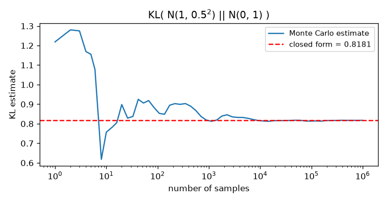
The Monte Carlo estimate averages \(\log q(x) - \log p(x)\) over samples \(x \sim q\) and converges by the law of large numbers from chapter 2. The closed form has no noise and is fast, so KL between Gaussians is always computed in closed form. In the VAE code of chapter 8, this formula becomes a single line:
# 인코더는 σ 대신 logvar = log σ² 를 출력한다 (σ² = exp(logvar) > 0 이 저절로 보장됨)
kl = 0.5 * torch.sum(mu.pow(2) + logvar.exp() - 1.0 - logvar) / batch   # 차원별 KL 을 모두 더해 그림 한 장당 평균
logvar.exp() is \(\sigma^2\), logvar is \(\log\sigma^2\), torch.sum(...) is the sum of per-dimension KLs, and / batch takes the average per image.
KL between categorical distributions
DreamerV2 and V3 (chapter 12) use several categorical distributions as latent variables instead of Gaussians. Categorical KL is computed directly from the definition \(\sum_k q_k\log(q_k/p_k)\). An example with \(q = (0.7, 0.2, 0.1)\) and the uniform distribution \(p = (\frac13, \frac13, \frac13)\):
\(\begin{align} D_{\mathrm{KL}}(q \,\|\, p) &= 0.7\log\frac{0.7}{1/3} + 0.2\log\frac{0.2}{1/3} + 0.1\log\frac{0.1}{1/3} \\ &= 0.7 \times 0.7419 + 0.2 \times (-0.5108) + 0.1 \times (-1.2040) = 0.5194 - 0.1022 - 0.1204 \\ &\approx 0.2968 = \log 3 - H(q) \end{align}\)
- Some terms can be negative, but the sum is always non-negative.
- \(H(q) = 0.2497 + 0.3219 + 0.2303 = 0.8018\) and \(\log 3 - 0.8018 = 0.2968\), which agrees with \(D_{\mathrm{KL}}(q \,\|\, u) = \log K - H(q)\).
- DreamerV2's latent state is "32 categorical variables with 32 classes each," so its KL is the sum of 32 categorical KLs (KLs of independent dimensions add up).
Mutual information
Mutual information measures how much two random variables tell about each other. It is the KL between the actual joint distribution and the distribution that assumes independence (the product of the marginals).
\(I(X; Y) = D_{\mathrm{KL}}\big(p(x, y) \,\|\, p(x)\,p(y)\big) = \sum_{x, y} p(x, y)\log\frac{p(x, y)}{p(x)\,p(y)}\)
It is \(I = 0\) under independence and positive otherwise. Using \(p(x, y)/p(y) = p(x \mid y)\), it can be rewritten in another form.
\(\begin{align} I(X;Y) &= \sum_{x,y} p(x,y)\log\frac{p(x \mid y)}{p(x)} \\ &= -\sum_x p(x)\log p(x) - \Big(-\sum_{x,y} p(x,y)\log p(x \mid y)\Big) \\ &= H(X) - H(X \mid Y) \end{align}\)
\(H(X \mid Y) = -\sum_{x,y}p(x,y)\log p(x \mid y) = \sum_y p(y)\big[-\sum_x p(x \mid y)\log p(x \mid y)\big]\) is the conditional entropy, the uncertainty about \(X\) that remains after knowing \(Y\) (the entropy for each case \(Y = y\), weighted by \(p(y)\)). Mutual information is the reduction in uncertainty gained by knowing \(Y\).
It is computed here with the weather–umbrella joint distribution from chapter 2.
def mutual_information() -> None:
    # 날씨 X(맑음/비) 와 우산 Y(안 씀/씀) 의 결합 분포
    joint = np.array([[0.45, 0.05],  # 맑음: 안 씀, 씀
                      [0.10, 0.40]])  # 비  : 안 씀, 씀
    px = joint.sum(axis=1, keepdims=True)  # 주변 분포 p(x) (행의 합)
    py = joint.sum(axis=0, keepdims=True)  # 주변 분포 p(y) (열의 합)
    mi = np.sum(joint * np.log(joint / (px * py)))
    print(f"[상호정보량] p(x) = {px.ravel().tolist()}, p(y) = {py.ravel().tolist()}")
    print(f"[상호정보량] I(X;Y) = {mi:.4f} nats   (독립이면 0)")
    indep = px * py  # 독립이라면 결합 분포는 곱이 된다
    print(f"[상호정보량] 독립인 결합 분포로 계산하면 I = {np.sum(indep * np.log(indep / (px * py))):.4f}")
[상호정보량] p(x) = [0.5, 0.5], p(y) = [0.55, 0.45]
[상호정보량] I(X;Y) = 0.2754 nats   (독립이면 0)
[상호정보량] 독립인 결합 분포로 계산하면 I = 0.0000
Checking by hand:
- \(H(X) = \log 2 = 0.6931\).
- On days without an umbrella, the weather distribution is \((0.45, 0.10)/0.55 = (0.818, 0.182)\) with entropy 0.4741; on days with one, it is \((0.05, 0.40)/0.45 = (0.111, 0.889)\) with entropy 0.3488.
- \(H(X \mid Y) = 0.55 \times 0.4741 + 0.45 \times 0.3488 = 0.4177\) and \(I = 0.6931 - 0.4177 = 0.2754\). Seeing the umbrella reduces the uncertainty about the weather by about 40%.
This tutorial does not use mutual information directly as a loss, but it appears often in representation learning papers, so it is also included in the glossary in chapter 14.
Preview of the ELBO
A latent variable model writes the probability of an observation \(x\) as an integral that marginalizes over the hidden \(z\) (this is the same as the observation \(o\) in chapter 00's notation; chapter 8 uses \(x\) following the convention of the VAE paper, so \(x\) is used here too).
\(p(x) = \int p(x \mid z)\,p(z)\,dz\)
This integral usually cannot be computed. So an arbitrary distribution \(q(z)\) is introduced (assuming \(q(z) \gt 0\)), and Jensen's inequality gives a lower bound on \(\log p(x)\).
\(\begin{align} \log p(x) &= \log\int q(z)\,\frac{p(x \mid z)\,p(z)}{q(z)}\,dz = \log \mathbb{E}_{z \sim q}\!\left[\frac{p(x \mid z)\,p(z)}{q(z)}\right] \\ &\ge \mathbb{E}_{z \sim q}\!\left[\log\frac{p(x \mid z)\,p(z)}{q(z)}\right] \\ &= \mathbb{E}_{z \sim q}[\log p(x \mid z)] + \mathbb{E}_{z \sim q}\!\left[\log\frac{p(z)}{q(z)}\right] \\ &= \underbrace{\mathbb{E}_{z \sim q}[\log p(x \mid z)]}_{\text{reconstruction term}} \;-\; \underbrace{D_{\mathrm{KL}}\big(q(z) \,\|\, p(z)\big)}_{\text{regularization term}} \;=:\; \text{ELBO} \end{align}\)
The first line multiplies the integrand by \(q(z)/q(z) = 1\), and the inequality comes from the concavity of \(\log\) (\(\log\mathbb{E}[Y] \ge \mathbb{E}[\log Y]\)). The right-hand side is called the evidence lower bound (ELBO). The first term is the log-likelihood from chapter 2 (the negative of the NLL), the second is computed with the closed-form Gaussian KL, and Jensen's inequality ties them together. Chapter 8 covers when this inequality becomes an equality, how to choose \(q\) (\(q_\phi(z \mid x)\)), and how to differentiate through \(\mathbb{E}_q\) (reparameterization).
Summary
- Information content \(-\log p\) is the only form that follows from the requirement that "surprises of independent events add up." Its unit is the nat (natural logarithm) or the bit.
- Entropy \(H(p) = \mathbb{E}_p[-\log p]\) is both the average surprise and the uncertainty. It is maximized at \(\log K\) by the uniform distribution, and for a Gaussian it is \(\frac12\log(2\pi e\sigma^2)\).
- Cross-entropy is \(H(p, q) = \mathbb{E}_p[-\log q]\), and KL is \(H(p, q) - H(p) = \mathbb{E}_p[\log(p/q)]\). Maximum likelihood is equivalent to minimizing \(D_{\mathrm{KL}}(p_{\text{data}} \,\|\, p_\theta)\).
- Jensen's inequality: for convex \(f\), \(f(\mathbb{E} X) \le \mathbb{E} f(X)\); for the concave \(\log\), \(\log\mathbb{E} X \ge \mathbb{E}\log X\). This proves \(D_{\mathrm{KL}} \ge 0\).
- Forward KL \(D_{\mathrm{KL}}(p \,\|\, q)\) covers the modes (matches mean and variance); reverse KL \(D_{\mathrm{KL}}(q \,\|\, p)\) seeks a single mode.
- The Gaussian KL is \(\log\frac{\sigma_2}{\sigma_1} + \frac{\sigma_1^2 + (\mu_1-\mu_2)^2}{2\sigma_2^2} - \frac12\); to the standard normal it is \(\frac12(\mu^2 + \sigma^2 - 1 - \log\sigma^2)\); for diagonal Gaussians it is the sum over dimensions.
- Mutual information is \(I(X;Y) = D_{\mathrm{KL}}(p(x,y) \,\|\, p(x)p(y)) = H(X) - H(X \mid Y)\).
- ELBO: \(\log p(x) \ge \mathbb{E}_q[\log p(x \mid z)] - D_{\mathrm{KL}}(q(z) \,\|\, p(z))\). This is the starting point of chapter 8.
Exercises
- 1. Entropy of one roll of a fair die
- It is uniform, so \(H = \log 6 \approx 1.792\) nats \(= \log_2 6 \approx 2.585\) bits. This is the maximum entropy a distribution with 6 outcomes can have.
- 2. KL in both directions for \(p = (0.5, 0.5)\), \(q = (0.9, 0.1)\)
- \(D_{\mathrm{KL}}(p \,\|\, q) = 0.5(-0.5878) + 0.5(1.6094) = 0.5108\), \(D_{\mathrm{KL}}(q \,\|\, p) = 0.9(0.5878) + 0.1(-1.6094) = 0.3681\). It is asymmetric.
- 3. \(D_{\mathrm{KL}}(\mathcal{N}(2, 1) \,\|\, \mathcal{N}(0, 1))\) and \(D_{\mathrm{KL}}(\mathcal{N}(0, 4) \,\|\, \mathcal{N}(0, 1))\)
- The first, by the special-case formula, is \(\frac12(4 + 1 - 1 - 0) = 2\). For the second, \(\sigma^2 = 4\), so it is \(\frac12(0 + 4 - 1 - \log 4) = \frac12(3 - 1.386) = 0.807\).
- 4. Proving arithmetic mean ≥ geometric mean with Jensen's inequality (positive \(a, b\))
- Since \(\log\) is concave, \(\log\frac{a + b}{2} \ge \frac12\log a + \frac12\log b = \log\sqrt{ab}\), and since \(\log\) is increasing, \(\frac{a+b}{2} \ge \sqrt{ab}\).
- 5. Shape of the maximum likelihood solution when the data distribution has two peaks but the model is a single Gaussian
- Maximum likelihood minimizes the forward KL \(D_{\mathrm{KL}}(p_{\text{data}} \,\|\, p_\theta)\). A small model probability where data exists is heavily penalized, so the result is a wide Gaussian covering both peaks (with its mean between them).
- 6. The \(q(z)\) that makes Jensen's inequality in the ELBO an equality
- If \(\frac{p(x \mid z)p(z)}{q(z)} = c\) (a constant), then \(q(z) \propto p(x, z)\), and normalizing gives \(q(z) = p(x, z)/p(x) = p(z \mid x)\), the true posterior. In that case \(c = p(x)\) and ELBO \(= \log p(x)\). Chapter 8 derives this again as the identity \(\log p(x) = \text{ELBO} + D_{\mathrm{KL}}(q \,\|\, p(z \mid x))\).
See also
- World Models:Tutorial
- World Models
- Information Theory
- Entropy
- Cross entropy
- Maximum likelihood estimation
- Normal distribution
- VAE