WorldModels:Tutorial:02-Probability
lastmod 2026-11-18created 2026-11-172 edits
Probability and maximum likelihood is Chapter 2 of the World Model tutorial. A World Model predicts the future as a probability distribution rather than a single number, and it is trained using the principle of maximum likelihood. This chapter starts from the basics of probability (distributions, conditional probability, Bayes' theorem, expectation and variance, the Gaussian) and derives the fact that mean squared error (MSE) and cross-entropy loss are both negative log-likelihood (NLL).
- Original: 02. Math ①: Probability and Maximum Likelihood
- Practice code:
code/ch02_probability.py(runs in a few seconds on a CPU, no GPU needed;--quickcuts the number of samples to 1/10) - Previous: 01. What Is a World Model? / Next: 03. Information Theory and KL Divergence
Why probability?
A World Model is a function that predicts the next state, but the world contains three kinds of uncertainty.
- Randomness in the world itself: as with dice, wind, or other people's choices, the outcome differs each time even in the same situation.
- Hidden information: a single image does not reveal the pendulum's velocity, so several different next frames look possible.
- The model's own ignorance: in situations it has never seen, the model cannot be certain either.
To say "the next state is probably near 0.3, but it could be 0.5" instead of "the next state is 0.3", we need a probability distribution that expresses how plausible each value is. The concepts in this chapter are used later as follows.
| Concept in this chapter | Where it is used |
| Conditional probability \(p(y \mid x)\) | World Model \(p_\theta(s_{t+1} \mid s_t, a_t)\), policy \(\pi(a \mid s)\) (all chapters) |
| Bayes' theorem | Encoder \(q_\phi(z \mid o)\) that infers the hidden state from an image (Chapter 8, Chapter 11), belief states in POMDPs (Chapter 5) |
| Expectation, Monte Carlo | Expected return (Chapter 5), ELBO estimation (Chapter 8), λ-return (Chapter 12) |
| Gaussian, \(\mu + \sigma\epsilon\) | Stochastic dynamics (Chapter 7), VAE reparameterization (Chapter 8), RSSM (Chapter 11), action distributions (Chapter 12) |
| Maximum likelihood, negative log-likelihood | Training loss of every World Model |
Random variables and probability distributions
A random variable is a number assigned to the outcome of a random experiment. By convention, a random variable is written in uppercase as \(X\) and the value it takes in lowercase as \(x\), but when the context is clear, both are often written in lowercase without distinction.
Probability mass function
If the values are countable and separate from one another, the random variable is discrete. The function that gives the probability of each value is the probability mass function (PMF), written \(P(X = x)\) or \(p(x)\).
\(0 \le p(x) \le 1, \qquad \sum_{x} p(x) = 1\)
For a fair die, \(p(1) = \cdots = p(6) = \tfrac{1}{6}\).
Probability density function
If the values range over the real numbers, like the angle of a pendulum, the random variable is continuous. Because there are infinitely many possible values, the probability of any single point is 0, so we talk about the probability of an interval instead, and for this we use the probability density function (PDF).
\(P(a \le X \le b) = \int_a^b p(x)\,dx = \lim_{\Delta x \to 0} \sum_{i} p(x_i)\,\Delta x\)
The integral slices the interval into thin bars of width \(\Delta x\) and adds up their areas \(p(x)\,\Delta x\). The conditions on a density function are those of the PMF with the sum replaced by an integral.
\(p(x) \ge 0, \qquad \int_{-\infty}^{\infty} p(x)\,dx = 1\)
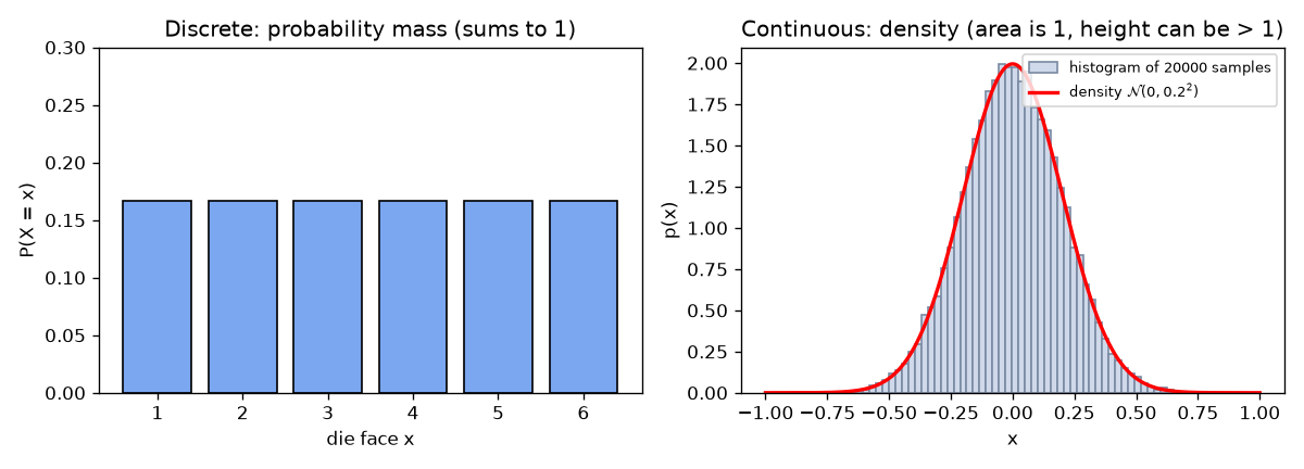
Caution: density is not probability. A probability mass cannot exceed 1, but a probability density can, because density is "probability per unit length". The uniform distribution on \([0, 0.5]\) has a constant density \(c\) inside the interval, and the area \(0.5\,c = 1\) gives \(c = 2\). The density is 2, but the area (the probability) is exactly 1.
The practice code confirms the same fact with a narrow Gaussian with \(\sigma = 0.2\). np.sum(pdf) * (grid[1] - grid[0]) is a Riemann sum that adds up height × width, that is, an approximation of the integral.
def gaussian_pdf(x, mu, sigma):
    """1차원 가우시안 밀도  N(x; μ, σ²) = 1/(σ√(2π)) · exp(-(x-μ)² / (2σ²))."""
    return np.exp(-((x - mu) ** 2) / (2 * sigma**2)) / (sigma * np.sqrt(2 * np.pi))


def density_can_exceed_one(rng: np.random.Generator, n: int, fig_dir: str) -> None:
    mu, sigma = 0.0, 0.2
    x = rng.normal(mu, sigma, size=n)  # μ + σ·ε 로 뽑는 것과 같다
    grid = np.linspace(-1, 1, 400)
    pdf = gaussian_pdf(grid, mu, sigma)
    area = np.sum(pdf) * (grid[1] - grid[0])  # 넓이 = Σ 높이 × 폭 (리만 합)
    # 격자에 정확한 0 은 없어서 pdf.max() 는 p(±0.0025) 이지만, p(0) = 1.9947 과 거의 같다.
    print(f"[밀도] 최댓값 p(0) = {pdf.max():.4f} (1 보다 크다!),  밑넓이 ≈ {area:.4f}")
Joint, marginal, and conditional probability
A World Model handles several variables together, such as the current state, the action, and the next state. As an example, take the proportions recorded over 100 days for the weather \(X\) (sunny, rain) and umbrella use \(Y\) (no umbrella, umbrella).
| No umbrella | Umbrella | Total (marginal \(p(x)\)) | |
| Sunny | 0.45 | 0.05 | 0.50 |
| Rain | 0.10 | 0.40 | 0.50 |
| Total (marginal \(p(y)\)) | 0.55 | 0.45 | 1.00 |
- Joint probability \(p(x, y)\)
- The probability that both events happen together. \(p(\text{rain}, \text{umbrella}) = 0.40\). The four inner cells of the table form the joint distribution, and they sum to 1.
- Marginal probability \(p(x)\)
- The probability obtained by summing over every case of the other variable to eliminate it. This computation is called marginalization. \(p(\text{rain}) = 0.10 + 0.40 = 0.50\). It is the value written in the margin of the table.
- Conditional probability \(p(y \mid x)\)
- The probability of \(y\) given that \(x\) has occurred. \(p(\text{umbrella} \mid \text{rain}) = 0.40 / 0.50 = 0.8\). A conditional probability also sums to 1 over \(y\) (\(0.2 + 0.8\)).
\(p(x) = \sum_{y} p(x, y) \quad \Big(\text{for continuous variables, } p(x) = \int p(x, y)\,dy\Big), \qquad p(y \mid x) = \frac{p(x, y)}{p(x)} \quad (p(x) \gt 0)\)
Product rule and chain rule
Multiplying both sides of the definition of conditional probability by \(p(x)\) gives the product rule. The second equality swaps the roles of \(x\) and \(y\).
\(p(x, y) = p(y \mid x)\, p(x) = p(x \mid y)\, p(y)\)
With three or more variables, applying the product rule repeatedly gives the chain rule. Apply it once treating \((x_1, x_2)\) as a single block, then once more to the remaining \(p(x_1, x_2)\).
\(\begin{align} p(x_1, x_2, x_3) &= p(x_3 \mid x_1, x_2)\; p(x_1, x_2) \\ &= p(x_1)\; p(x_2 \mid x_1)\; p(x_3 \mid x_1, x_2) \end{align}\)
\(p(x_1, \dots, x_T) = \prod_{t=1}^{T} p(x_t \mid x_1, \dots, x_{t-1})\)
When states follow one another in time, this formula says "the probability of the whole story = the product of the probabilities of each next scene, one scene at a time". Adding the Markov property from Chapter 5, \(p(s_{t+1} \mid s_1, \dots, s_t, a_1, \dots, a_t) = p(s_{t+1} \mid s_t, a_t)\), turns the probability of an episode into a product of the one-step transition probabilities that the World Model predicts. The sequential ELBO in Chapter 11 starts from this factorization.
Independence
Two random variables are independent if neither gives any information about the other.
\(p(x, y) = p(x)\, p(y) \quad\Longleftrightarrow\quad p(y \mid x) = p(y)\)
Substituting the left equation into the definition of conditional probability gives \(p(y \mid x) = p(x)p(y)/p(x) = p(y)\), so the two statements are equivalent. Weather and umbrella use are not independent, since \(p(\text{rain})\,p(\text{umbrella}) = 0.5 \times 0.45 = 0.225 \ne 0.40\). The results of two die rolls are independent. Maximum likelihood estimation relies on the assumption that "the data points are independent of each other".
Bayes' theorem
Bayes' theorem is a formula that inverts a conditional probability, expressing \(p(y \mid x)\) in terms of \(p(x \mid y)\). Take the two forms of the product rule, \(p(y \mid x)\, p(x) = p(x, y) = p(x \mid y)\, p(y)\), divide both ends by \(p(x)\), and expand the denominator by marginalization.
\(p(y \mid x) = \frac{p(x \mid y)\, p(y)}{p(x)} = \frac{p(x \mid y)\, p(y)}{\sum_{y'} p(x \mid y')\, p(y')}\)
Treating \(y\) as the hidden cause and \(x\) as the observed evidence, the parts are named as follows.
- \(p(y)\): prior. The belief before seeing the evidence.
- \(p(x \mid y)\): likelihood. The probability of the evidence \(x\) if the cause is \(y\).
- \(p(x)\): evidence. The overall probability of \(x\) when the cause is unknown.
- \(p(y \mid x)\): posterior. The belief revised after seeing the evidence.
If something else, \(C\), is already known, the theorem still holds as long as the same condition \(C\) is attached to every probability. Chapter 5 uses this form to update a belief with a new observation while conditioning on "the history so far, \(C\)".
\(p(A \mid B, C) = \frac{p(B \mid A, C)\, p(A \mid C)}{p(B \mid C)}\)
Example: what a positive test result means
A certain disease affects 1 in 100 people. The test comes out positive 99% of the time when the disease is present, and 5% of the time even for healthy people.
\(\begin{align} p(\text{positive}) &= 0.99 \times 0.01 + 0.05 \times 0.99 = 0.0099 + 0.0495 = 0.0594 \\ p(\text{disease} \mid \text{positive}) &= \frac{0.99 \times 0.01}{0.0594} = \frac{0.0099}{0.0594} \approx 0.1667 \end{align}\)
Even though the test is 99% accurate, only about 17% of the people who test positive actually have the disease. Counting 10,000 people, 99 of the 100 patients test positive and 495 of the 9,900 healthy people test positive, giving \(99/594 \approx 0.167\). Because the prior is small, false positives far outnumber true positives. A simulation with 1 million people gives the same value.
def bayes_example(rng: np.random.Generator, n_people: int) -> None:
    """병 검사 예제: 양성이 나왔을 때 정말 병이 있을 확률은?"""
    p_d = 0.01  # P(병)          : 100 명 중 1 명
    p_pos_d = 0.99  # P(양성 | 병)   : 병이 있으면 99% 양성
    p_pos_nd = 0.05  # P(양성 | 건강) : 건강해도 5% 는 양성(오진)

    # 공식: P(병 | 양성) = P(양성 | 병) P(병) / P(양성)
    p_pos = p_pos_d * p_d + p_pos_nd * (1 - p_d)  # 주변화: 병인 경우 + 건강한 경우
    posterior = p_pos_d * p_d / p_pos
    print(f"[베이즈] 공식     P(양성) = {p_pos:.4f},  P(병 | 양성) = {posterior:.4f}")

    # 시뮬레이션: 가상의 사람을 많이 만들어 실제로 세어 본다.
    sick = rng.random(n_people) < p_d  # 각 사람이 병이 있는지
    u = rng.random(n_people)
    positive = np.where(sick, u < p_pos_d, u < p_pos_nd)  # 병 여부에 따라 양성 확률이 다르다
    print(f"[베이즈] 시뮬레이션 양성 {positive.sum()} 명 중 병 {np.sum(sick & positive)} 명"
          f" → P(병 | 양성) ≈ {np.sum(sick & positive) / positive.sum():.4f}")
Bayes' theorem in World Models
In a World Model that sees images, the hidden cause is the latent state \(z\) (e.g., the angle of the pendulum) and the evidence is the image \(o\). What we want is the posterior \(p(z \mid o)\), but the integral in the denominator \(p(o) = \int p(o \mid z) p(z)\,dz\) cannot be computed. So Chapter 8 approximates the posterior with a neural network \(q_\phi(z \mid o)\) (following the convention of the VAE paper, Chapter 8 writes the observation as \(x\) instead of \(o\)).
Expectation
The expectation is a probability-weighted average: the value that the average of the outcomes approaches when the same experiment is repeated a very large number of times.
\(\mathbb{E}[X] = \sum_x x\, p(x) \quad \Big(\text{for continuous variables, } \int x\, p(x)\,dx\Big), \qquad \mathbb{E}_{x \sim p}[f(x)] = \sum_x f(x)\, p(x)\)
For a die, \(\mathbb{E}[X] = 21/6 = 3.5\) and \(\mathbb{E}[X^2] = 91/6 \approx 15.17\). The value 3.5 can never actually come up (the "average turns into an impossible value" problem from Chapter 1).
Linearity
Constant factors and sums can be pulled out of the expectation.
\(\begin{align} \mathbb{E}[aX + b] &= \sum_x (a x + b)\, p(x) = a \sum_x x\, p(x) + b \sum_x p(x) = a\,\mathbb{E}[X] + b \\ \mathbb{E}[X + Y] &= \sum_x \sum_y (x + y)\, p(x, y) = \sum_x x \sum_y p(x, y) + \sum_y y \sum_x p(x, y) \\ &= \sum_x x\, p(x) + \sum_y y\, p(y) = \mathbb{E}[X] + \mathbb{E}[Y] \end{align}\)
The second derivation uses only marginalization and no independence assumption. The expectation of a sum always splits. Products are different: \(\mathbb{E}[XY] = \mathbb{E}[X]\,\mathbb{E}[Y]\) holds when \(X\) and \(Y\) are independent, because the two sums separate only when the joint probability factors into \(p(x)p(y)\).
Conditional expectation and the law of total expectation
The conditional expectation is an expectation with the conditional probability in place of the probability.
\(\mathbb{E}[X \mid Y = y] = \sum_x x\, p(x \mid y)\)
Weighting the average of each case by the probability of that case and summing gives the overall average. This is the law of total expectation. It follows from marginalization, the product rule, and swapping the order of summation.
\(\begin{align} \mathbb{E}[X] &= \sum_x x \sum_y p(x, y) = \sum_x x \sum_y p(x \mid y)\, p(y) \\ &= \sum_y p(y) \sum_x x\, p(x \mid y) = \sum_y p(y)\; \mathbb{E}[X \mid Y = y] \end{align}\)
In the weather and umbrella table, let \(Y = 1\) when an umbrella is used and \(Y = 0\) when it is not. Then \(\mathbb{E}[Y \mid \text{sunny}] = 0.05/0.50 = 0.1\), \(\mathbb{E}[Y \mid \text{rain}] = 0.40/0.50 = 0.8\), and \(\mathbb{E}[Y] = 0.5 \times 0.1 + 0.5 \times 0.8 = 0.45 = p(\text{umbrella})\). The Bellman equation in Chapter 5 (splitting cases by "what the first action was") and the ensembles in Chapter 7 (splitting cases by "which model was drawn") use this law.
Variance and standard deviation
Variance measures how far the values are spread out from the mean. Writing \(\mu = \mathbb{E}[X]\),
\(\operatorname{Var}[X] = \mathbb{E}\big[(X - \mu)^2\big], \qquad \sigma = \sqrt{\operatorname{Var}[X]}\ \ \text{(standard deviation)}\)
Expanding and applying linearity gives a formula that is convenient for computation.
\(\operatorname{Var}[X] = \mathbb{E}[X^2] - 2\mu\,\mathbb{E}[X] + \mu^2 = \mathbb{E}[X^2] - (\mathbb{E}[X])^2\)
That is, "the mean of the square − the square of the mean". Since variance is nonnegative, \(\mathbb{E}[X^2] \ge (\mathbb{E}[X])^2\) always holds (an instance of Jensen's inequality from Chapter 3). For a die, \(\operatorname{Var}[X] = 91/6 - 3.5^2 = 2.9167\ (= 35/12)\) and \(\sigma \approx 1.708\).
Variance has the following two properties.
\(\begin{align} \operatorname{Var}[aX + b] &= \mathbb{E}\big[(aX + b - a\mu - b)^2\big] = \mathbb{E}\big[a^2 (X - \mu)^2\big] = a^2\, \operatorname{Var}[X] \\ \operatorname{Var}[X + Y] &= \mathbb{E}[(X - \mu_X)^2] + \mathbb{E}[(Y - \mu_Y)^2] + 2\,\mathbb{E}[(X - \mu_X)(Y - \mu_Y)] \end{align}\)
- A shift \(b\) does not affect the spread, and scaling by \(a\) multiplies the variance by \(a^2\).
- The last expectation is the covariance \(\operatorname{Cov}[X, Y]\). If the variables are independent, it splits into \(\mathbb{E}[X - \mu_X]\,\mathbb{E}[Y - \mu_Y] = 0 \times 0 = 0\), so \(\operatorname{Var}[X + Y] = \operatorname{Var}[X] + \operatorname{Var}[Y]\). The same holds for \(N\) variables.
Monte Carlo estimation and the law of large numbers
Computing an expectation exactly requires summing or integrating over every \(x\), which is usually impossible. Instead, we draw \(N\) samples from the distribution and average them. This is Monte Carlo estimation.
\(\mathbb{E}_{x \sim p}[f(x)] \approx \hat{\mu}_N = \frac{1}{N} \sum_{i=1}^{N} f(x_i), \qquad x_i \sim p \ \text{(independent)}\)
Let \(Y_i = f(x_i)\), \(\mu = \mathbb{E}[Y_i]\), and \(\sigma^2 = \operatorname{Var}[Y_i]\). Then two things hold.
\(\begin{align} \mathbb{E}[\hat{\mu}_N] &= \frac{1}{N} \sum_{i=1}^N \mathbb{E}[Y_i] = \frac{1}{N} \cdot N\mu = \mu \\ \operatorname{Var}[\hat{\mu}_N] &= \frac{1}{N^2}\, \operatorname{Var}\Big[\sum_{i=1}^N Y_i\Big] = \frac{1}{N^2} \cdot N \sigma^2 = \frac{\sigma^2}{N} \end{align}\)
- First line: the mean of the estimate is exactly the true value, so the estimator has no bias (it is unbiased).
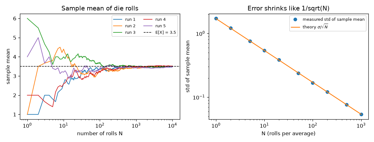
- Second line: uses \(\operatorname{Var}[aX] = a^2\operatorname{Var}[X]\) and the fact that variances of independent samples add. The standard deviation of the estimate is \(\sigma/\sqrt{N}\). Because it is inversely proportional to \(\sqrt{N}\), halving the error takes 4 times as many samples.
The fact that the sample mean approaches the expectation as \(N \to \infty\) is called the law of large numbers, and the variance formula above explains why. The results checked with a die (\(\sigma = 1.708\)) are shown below. The experimental values are the standard deviation measured over 4,000 sample means, and the running mean is computed with np.cumsum(rolls) / np.arange(1, n_rolls + 1) (the lln section).
| \(N\) | Experimental standard deviation | Theoretical \(\sigma/\sqrt{N}\) |
| 10 | 0.5440 | 0.5401 |
| 100 | 0.1681 | 0.1708 |
| 1000 | 0.0537 | 0.0540 |
Mini-batch training (Chapter 4) is also Monte Carlo: instead of the mean loss over the whole dataset, it uses the mean loss of a single randomly drawn batch. The VAE in Chapter 8 estimates \(\mathbb{E}_{q}[\log p(o \mid z)]\) with a single sample, and training still works because the errors average out over many iterations.
Gaussian distribution
The continuous distribution used most in deep learning and World Models is the Gaussian distribution, also called the normal distribution. The density of a Gaussian with mean \(\mu\) and variance \(\sigma^2\) is as follows.
\(\mathcal{N}(x;\, \mu, \sigma^2) = \frac{1}{\sigma\sqrt{2\pi}} \exp\!\left(-\frac{(x - \mu)^2}{2\sigma^2}\right)\)
The \(x\) before the semicolon is the point where the density is evaluated, and what follows are the parameters of the distribution. When referring to the distribution itself, as in \(x \sim \mathcal{N}(\mu, \sigma^2)\), the \(x;\) is omitted.
- \((x - \mu)^2\): the squared distance from the mean. It is 0 at the mean and symmetric on both sides.
- \(\dfrac{(x-\mu)^2}{2\sigma^2}\): measures the distance in units of \(\sigma\). A larger \(\sigma\) spreads the curve wider.
- \(\exp(-\,\cdot\,)\): equals 1 at 0 and drops quickly toward 0 as its argument grows. This produces the bell shape.
- \(\dfrac{1}{\sigma\sqrt{2\pi}}\): the normalization constant that makes the area under the curve equal to 1.
Numerical examples: \(\mathcal{N}(0; 0, 1) = 1/\sqrt{2\pi} \approx 0.3989\), \(\mathcal{N}(1; 0, 1) = 0.3989 \times e^{-0.5} \approx 0.2420\), \(\mathcal{N}(0; 0, 0.04) = 1/(0.2\sqrt{2\pi}) \approx 1.995\).
Deriving the normalization constant
Multiply \(I = \int_{-\infty}^{\infty} e^{-x^2/2}\,dx\) by itself to view it as an integral over the whole plane, and change to polar coordinates \(x = r\cos\alpha,\ y = r\sin\alpha,\ dx\,dy = r\,dr\,d\alpha\).
\(\begin{align} I^2 &= \int\!\!\int e^{-(x^2 + y^2)/2}\,dx\,dy = \int_0^{2\pi} \int_0^{\infty} e^{-r^2/2}\; r\,dr\,d\alpha \\ \int_0^\infty e^{-r^2/2}\,r\,dr &= \int_0^\infty e^{-v}\,dv = \Big[-e^{-v}\Big]_0^\infty = 1 \qquad (v = r^2/2,\ dv = r\,dr) \\ I^2 &= \int_0^{2\pi} 1\; d\alpha = 2\pi \quad\Rightarrow\quad I = \sqrt{2\pi} \end{align}\)
A general Gaussian reduces to the same integral with the substitution \(t = (x - \mu)/\sigma\), \(dx = \sigma\,dt\).
\(\int_{-\infty}^{\infty} \exp\!\left(-\frac{(x-\mu)^2}{2\sigma^2}\right) dx = \sigma \int_{-\infty}^{\infty} e^{-t^2/2}\,dt = \sigma\sqrt{2\pi}\)
So putting \(1/(\sigma\sqrt{2\pi})\) in front makes the area exactly 1.
Standard normal distribution and sampling
The Gaussian with \(\mu = 0\) and \(\sigma = 1\) is the standard normal distribution, and a value drawn from it is written \(\epsilon \sim \mathcal{N}(0, 1)\). A sample from any Gaussian can be drawn as follows. This is the basis of the reparameterization used in the Chapter 8 VAE.
\(x = \mu + \sigma\,\epsilon, \qquad \epsilon \sim \mathcal{N}(0, 1) \quad\Longrightarrow\quad x \sim \mathcal{N}(\mu, \sigma^2)\)
Write the standard normal density as \(\varphi(t) = \frac{1}{\sqrt{2\pi}} e^{-t^2/2}\). First, we show that \(\epsilon\) has mean 0 and variance 1.
- \(\mathbb{E}[\epsilon] = \int t\,\varphi(t)\,dt = 0\): because \(\varphi\) is symmetric, the areas of \(t\varphi(t)\) on the left and right cancel.
- Since \(\varphi'(t) = -t\,\varphi(t)\), write \(t^2\varphi = (-t)\,\varphi'\) and integrate by parts (\(u = -t,\ v = \varphi\)).
\(\mathbb{E}[\epsilon^2] = \int (-t)\,\varphi'(t)\,dt = \Big[-t\,\varphi(t)\Big]_{-\infty}^{\infty} + \int \varphi(t)\,dt = 0 + 1 = 1, \qquad \operatorname{Var}[\epsilon] = 1 - 0 = 1\)
Now check \(x = \mu + \sigma\epsilon\). Linearity and \(\operatorname{Var}[aX + b] = a^2\operatorname{Var}[X]\) give the mean and variance \(\mathbb{E}[x] = \mu\) and \(\operatorname{Var}[x] = \sigma^2\). The shape is confirmed by differentiating the cumulative distribution function \(\Phi(t) = \int_{-\infty}^{t}\varphi\).
\(\begin{align} P(x \le c) &= P\!\left(\epsilon \le \frac{c - \mu}{\sigma}\right) = \Phi\!\left(\frac{c-\mu}{\sigma}\right) \\ p_x(c) &= \frac{d}{dc}\,\Phi\!\left(\frac{c-\mu}{\sigma}\right) = \varphi\!\left(\frac{c-\mu}{\sigma}\right) \cdot \frac{1}{\sigma} = \frac{1}{\sigma\sqrt{2\pi}} \exp\!\left(-\frac{(c-\mu)^2}{2\sigma^2}\right) = \mathcal{N}(c;\, \mu, \sigma^2) \end{align}\)
Stretching (\(\times\sigma\)) and shifting (\(+\mu\)) a standard normal sample gives a sample from the desired Gaussian.
68 – 95 – 99.7: for a Gaussian, about 68% of values fall within \(\mu \pm \sigma\), about 95% within \(\mu \pm 2\sigma\), and about 99.7% within \(\mu \pm 3\sigma\). This is why \(\sigma\) is read as the size of the uncertainty, meaning "the prediction can wobble by about this much". It is also why Chapter 7 has the World Model predict \(\sigma\) along with \(\mu\).
Diagonal Gaussian
What a World Model predicts is a vector (3 values for the pendulum, around 30 for latent variables). The most common approach is the diagonal Gaussian, which treats each dimension as an independent Gaussian. Because the dimensions are independent, the joint density is a product. \(\operatorname{diag}(\sigma^2)\) is the covariance matrix with the variances \(\sigma_1^2, \dots, \sigma_D^2\) on the diagonal and all other entries (the covariances) set to 0.
\(\mathcal{N}(x;\, \mu, \operatorname{diag}(\sigma^2)) = \prod_{d=1}^{D} \mathcal{N}(x_d;\, \mu_d, \sigma_d^2) = \frac{1}{(2\pi)^{D/2} \prod_d \sigma_d} \exp\!\left(-\sum_{d=1}^{D} \frac{(x_d - \mu_d)^2}{2\sigma_d^2}\right)\)
Log density
In practice, computations use the log density instead of the density. With the properties of logarithms, \(\log(ab) = \log a + \log b\), \(\log(a/b) = \log a - \log b\), \(\log(a^k) = k\log a\), and \(\log(e^u) = u\), products, quotients, and exponents all turn into additions.
\(\log \mathcal{N}(x; \mu, \sigma^2) = -\frac12\log(2\pi) - \log\sigma - \frac{(x-\mu)^2}{2\sigma^2}\)
The three terms are a constant (\(\tfrac12\log(2\pi) \approx 0.9189\)), a penalty on the size of \(\sigma\), and a penalty on the distance from the mean. With \(x = 1, \mu = 0, \sigma = 1\), this gives \(-0.9189 - 0 - 0.5 = -1.4189\), and \(e^{-1.4189} = 0.2420\) matches the density computed earlier. The log density of a diagonal Gaussian is the sum of the log densities of the individual dimensions.
\(\log \mathcal{N}(x;\, \mu, \operatorname{diag}(\sigma^2)) = -\frac{D}{2}\log(2\pi) - \sum_{d=1}^D \log\sigma_d - \sum_{d=1}^D \frac{(x_d - \mu_d)^2}{2\sigma_d^2}\)
Example: with \(D = 2\), \(x = (1, 0)\), \(\mu = (0, 0)\), and \(\sigma = (1, 2)\), the result is \(-1.8379 - 0.6931 - 0.5 = -3.0310\).
Likelihood and maximum likelihood estimation
Given data \(x_1, \dots, x_N\) and a model distribution \(p_\theta(x)\) determined by parameters \(\theta\), a good \(\theta\) is one that makes the observed data most plausible. If the data are assumed to be independent and identically distributed (i.i.d.), the probability of the whole dataset is a product. Viewed as a function of \(\theta\), this product is the likelihood, and finding the \(\theta\) that maximizes the likelihood is maximum likelihood estimation (MLE).
\(L(\theta) = p_\theta(x_1, \dots, x_N) = \prod_{i=1}^{N} p_\theta(x_i)\)
Why take the logarithm
- Numbers do not vanish. The product of 1,000 data points with probability 0.1 each is \(10^{-1000}\), but float64 cannot properly represent numbers smaller than about \(10^{-308}\) and turns anything smaller than about \(10^{-324}\) into 0. Taking the logarithm gives \(1000 \times \log 0.1 = -2302.6\).
- Products become sums. \(\log \prod_i p_\theta(x_i) = \sum_i \log p_\theta(x_i)\). Sums are easy both to differentiate and to split into mini-batches.
- The answer does not change. Since \(\log\) is an increasing function, the same \(\theta\) maximizes both \(L(\theta)\) and \(\log L(\theta)\).
Deep learning conventionally minimizes, so the sign is flipped and the negative log-likelihood (NLL) is used as the loss. Multiplying by \(1/N\) does not change the optimal \(\theta\), and taking the mean keeps the loss on a similar scale regardless of the number of data points.
\(\hat\theta_{\text{MLE}} = \operatorname*{arg\,max}_\theta \sum_{i=1}^N \log p_\theta(x_i) = \operatorname*{arg\,min}_\theta \left(-\frac{1}{N}\sum_{i=1}^N \log p_\theta(x_i)\right)\)
Example 1: a coin (Bernoulli)
The distribution with probability \(p\) for heads (\(x = 1\)) and \(1 - p\) for tails (\(x = 0\)) is the Bernoulli distribution. If \(N\) tosses produce \(k\) heads,
\(\begin{align} L(p) &= p^{k}\,(1 - p)^{N - k}, \qquad \log L(p) = k \log p + (N - k)\log(1 - p) \\ \frac{d}{dp}\log L(p) &= \frac{k}{p} - \frac{N - k}{1 - p} = 0 \;\Rightarrow\; k(1 - p) = (N - k)\,p \;\Rightarrow\; \hat p = \frac{k}{N} \end{align}\)
The maximum likelihood estimate is "the fraction of heads". With 7 heads in 10 tosses, \(\hat p = 0.7\).
Example 2: Gaussian
Summing the log density over the data points gives the log-likelihood
\(\log L(\mu, \sigma) = -\frac{N}{2}\log(2\pi) - N\log\sigma - \frac{1}{2\sigma^2}\sum_{i=1}^N (x_i - \mu)^2\)
Take the partial derivatives with respect to \(\mu\) and \(\sigma\) and set each to 0.
\(\begin{align} \frac{\partial \log L}{\partial \mu} &= \frac{1}{\sigma^2}\sum_{i=1}^N (x_i - \mu) = 0 \;\Rightarrow\; \hat\mu = \frac{1}{N}\sum_{i=1}^N x_i \\ \frac{\partial \log L}{\partial \sigma} &= -\frac{N}{\sigma} + \frac{1}{\sigma^3}\sum_{i=1}^N (x_i - \mu)^2 = 0 \;\Rightarrow\; \hat\sigma^2 = \frac{1}{N}\sum_{i=1}^N (x_i - \hat\mu)^2 \end{align}\)
The MLE of the mean is the sample mean, and the MLE of the variance is the sample variance. The second derivative with respect to \(\mu\) is \(-N/\sigma^2 \lt 0\), so this point is a maximum. In statistics, the sample variance is divided by \(N-1\) because the MLE, which divides by \(N\), comes out slightly smaller than the true variance on average (it is biased). When \(N\) is large the difference is negligible, so deep learning usually ignores it.
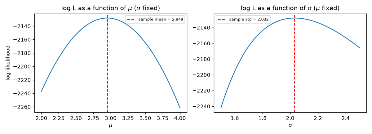
The code draws 1,000 samples from a Gaussian with true \(\mu = 3\) and \(\sigma = 2\) and compares three methods: the closed-form formula, grid search, and gradient descent (the plotting part of the mle section is omitted).
def gaussian_log_likelihood(x: np.ndarray, mu: float, sigma: float) -> float:
    """log L(μ, σ) = Σ_i log N(x_i; μ, σ²) = -N/2·log(2π) - N·log σ - Σ(x_i-μ)²/(2σ²)."""
    n = len(x)
    return -0.5 * n * math.log(2 * math.pi) - n * math.log(sigma) - np.sum((x - mu) ** 2) / (2 * sigma**2)


def gaussian_mle(rng: np.random.Generator, n: int, fig_dir: str) -> None:
    true_mu, true_sigma = 3.0, 2.0
    x = rng.normal(true_mu, true_sigma, size=n)

    # 풀이 상자에서 미분으로 구한 답
    mu_hat = x.mean()  # μ̂ = (1/N) Σ x_i
    var_hat = np.mean((x - mu_hat) ** 2)  # σ̂² = (1/N) Σ (x_i - μ̂)²
    sigma_hat = math.sqrt(var_hat)
    print(f"[MLE] 진짜 μ={true_mu}, σ={true_sigma}  /  공식 μ̂={mu_hat:.4f}, σ̂={sigma_hat:.4f}")

    # 확인 1: 격자에서 로그 가능도가 가장 큰 곳을 찾아본다.
    mus = np.linspace(2.0, 4.0, 401)
    sigmas = np.linspace(1.5, 2.5, 401)
    ll_mu = np.array([gaussian_log_likelihood(x, m, sigma_hat) for m in mus])
    ll_sigma = np.array([gaussian_log_likelihood(x, mu_hat, s) for s in sigmas])
    print(f"[MLE] 격자 탐색   μ*={mus[ll_mu.argmax()]:.4f}, σ*={sigmas[ll_sigma.argmax()]:.4f}")

    # 확인 2: 경사 하강(4장에서 배울 방법, 여기서는 Adam)으로 NLL 을 내려 본다 (= 로그 가능도를 올린다).
    xt = torch.tensor(x)
    mu_p = torch.tensor(0.0, requires_grad=True)
    log_sigma_p = torch.tensor(0.0, requires_grad=True)  # σ > 0 을 지키려고 log σ 를 학습한다
    opt = torch.optim.Adam([mu_p, log_sigma_p], lr=0.05)
    for _ in range(2000):
        sigma_p = log_sigma_p.exp()
        nll = (0.5 * math.log(2 * math.pi) + log_sigma_p + (xt - mu_p) ** 2 / (2 * sigma_p**2)).mean()
        opt.zero_grad()
        nll.backward()
        opt.step()
    print(f"[MLE] 경사 하강   μ*={mu_p.item():.4f}, σ*={log_sigma_p.exp().item():.4f}")
[MLE] 진짜 μ=3.0, σ=2.0  /  공식 μ̂=2.9492, σ̂=2.0321
[MLE] 격자 탐색   μ*=2.9500, σ*=2.0325
[MLE] 경사 하강   μ*=2.9492, σ*=2.0321
- All three methods give the same answer. It differs slightly from the true values (3, 2) because there are only 1,000 samples (the Monte Carlo \(\sigma/\sqrt{N}\) error).
- Since \(\sigma\) must always be positive, the code learns
log_sigma_pand builds \(\sigma\) withexp(). Whatever real number \(\log\sigma\) takes, \(\sigma = e^{\log\sigma} \gt 0\) is guaranteed. World Models use the same trick when predicting variance (Chapters 7 and 8). - The loss line is a direct transcription of the Gaussian NLL derived above.
- Figure: Figure 2-3. Log-likelihood curves as functions of μ and σ. The peaks lie at the sample mean and the sample standard deviation
What loss functions really are: negative log-likelihood
Deep learning models and World Models learn the conditional distribution \(p_\theta(y \mid x)\) of an output \(y\) given an input \(x\). For a World Model, \(x = (s_t, a_t)\) and \(y = s_{t+1}\). The neural network outputs the parameters of the distribution (e.g., the mean), and the NLL over the data \((x_i, y_i)\) is minimized. The familiar loss functions are all this NLL.
=== MSE = Gaussian NLL === Consider a model \(p_\theta(y \mid x) = \mathcal{N}(y;\, f_\theta(x), \sigma^2)\) in which a neural network \(f_\theta(x)\) outputs the mean and the standard deviation is fixed at \(\sigma\).
\(\begin{align} \text{NLL}(\theta) &= \frac{1}{N}\sum_{i=1}^N \left[\frac12\log(2\pi) + \log\sigma + \frac{(y_i - f_\theta(x_i))^2}{2\sigma^2}\right] \\ &= \frac{1}{2\sigma^2} \cdot \underbrace{\frac{1}{N}\sum_{i=1}^N (y_i - f_\theta(x_i))^2}_{\text{MSE}(\theta)} + \underbrace{\frac12\log(2\pi) + \log\sigma}_{\text{constant independent of } \theta} \end{align}\)
Multiplying by a positive constant or adding a constant does not move the location of the minimum, so \(\operatorname*{arg\,min}_\theta \text{NLL}(\theta) = \operatorname*{arg\,min}_\theta \text{MSE}(\theta)\). Training with MSE = training a fixed-variance Gaussian model by maximum likelihood. With \(\sigma = 1\), \(\text{NLL} = \text{MSE}/2 + 0.9189\).
Chapter 6 trains the pendulum World Model with MSE, which amounts to assuming that "the next state is a Gaussian that always wobbles around the prediction with the same width (\(\sigma\))". The limitation is that the width is treated as the same where prediction is easy and where it is hard; in Chapter 7, the neural network predicts \(\sigma\) as well.
Learning σ as well
When \(\sigma\) is learned, the \(\log\sigma\) term in the NLL comes back into play. For a single data point, differentiating \(\ell(\sigma) = \log\sigma + \frac{\delta^2}{2\sigma^2}\) (where \(\delta\) is the prediction error) gives
\(\frac{d\ell}{d\sigma} = \frac{1}{\sigma} - \frac{\delta^2}{\sigma^3} = 0 \;\Rightarrow\; \sigma^2 = \delta^2\)
The model learns to increase \(\sigma\) where the error is large and decrease it where the error is small. The \(\log\sigma\) term is a penalty that keeps the model from blindly inflating \(\sigma\) whenever it is unsure, and the \(\delta^2/(2\sigma^2)\) term punishes shrinking \(\sigma\) to look confident and then being wrong. The balance between these two forces produces honest uncertainty.
=== Binary cross-entropy = Bernoulli NLL === When the output is 0 or 1 (is the pixel on? has the episode ended?), we use a Bernoulli model in which the neural network outputs the "probability of 1", \(p = f_\theta(x) \in (0, 1)\). A single expression covers both cases, giving \(p\) when \(y = 1\) and \(1 - p\) when \(y = 0\).
\(\begin{align} p_\theta(y \mid x) &= p^{\,y}\,(1 - p)^{1 - y}, \qquad y \in \{0, 1\} \\ \text{BCE} &= -\frac{1}{N}\sum_{i=1}^N \Big[y_i \log p_i + (1 - y_i)\log(1 - p_i)\Big] \end{align}\)
This is the same formula as PyTorch's F.binary_cross_entropy. With targets \(y = (1, 0, 1, 1)\) and model probabilities \(p = (0.9, 0.2, 0.6, 0.99)\), the terms are 0.1054, 0.2231, 0.5108, and 0.0101, and the mean is \(0.8494/4 = 0.2123\). The VAE in Chapter 8 treats each pixel of an image as such a Bernoulli variable to compute the reconstruction loss.
=== Cross-entropy = categorical NLL === When the output is one of \(K\) categories, the neural network outputs a score for each category that can be any real number, \(l_1, \dots, l_K\) (the logits), and converts them into probabilities with softmax.
\(\pi_k = \operatorname{softmax}(l)_k = \frac{e^{l_k}}{\sum_{j=1}^{K} e^{l_j}}\)
If the correct category is \(y\), the likelihood is \(\pi_y\), and \(-\log \pi_y = -l_y + \log\sum_j e^{l_j}\).
\(\text{CE} = \frac{1}{N}\sum_{i=1}^N \Big(-l^{(i)}_{y_i} + \log\sum_{j=1}^K e^{l^{(i)}_j}\Big)\)
This is the formula that PyTorch's F.cross_entropy(logits, target) computes (Cross entropy); it takes logits, not probabilities, as input.
\(\log\sum_j e^{l_j}\) is called log-sum-exp (LSE). If a logit is as large as 1000, \(e^{1000}\) overflows, so the largest logit \(m\) is subtracted before computing. All the exponents are then at most 0, which is safe. The mixture density network in Chapter 9 uses this trick directly.
\(\log\sum_j e^{l_j} = m + \log\sum_j e^{l_j - m}\)
Numerical example: with logits \((2.0, 1.0, 0.1)\) and correct class 0, \(e^2 = 7.389\), \(e^1 = 2.718\), \(e^{0.1} = 1.105\), and the sum 11.212 gives \(\pi_0 = 0.659\) and a loss of 0.417. With logits \((0.5, 2.5, 0.3)\) and correct class 2, \(\pi_2 = 1.350/15.181 = 0.0889\) and the loss is 2.420. The mean of the two is 1.4185.
Checking in code
def losses_are_nll(rng: np.random.Generator) -> None:
    # (1) 회귀: σ = 1 로 고정한 가우시안 NLL 과 MSE 의 관계
    y = torch.tensor(rng.normal(size=8))  # 정답
    y_hat = y + torch.tensor(rng.normal(scale=0.5, size=8))  # 모델의 예측 (조금 틀림)
    sigma = 1.0
    nll = (0.5 * math.log(2 * math.pi) + math.log(sigma) + (y - y_hat) ** 2 / (2 * sigma**2)).mean()
    mse = F.mse_loss(y_hat, y)
    print(f"[손실] 가우시안 NLL = {nll.item():.6f}")
    print(f"[손실] MSE/2 + ½log(2π) = {(mse / 2 + 0.5 * math.log(2 * math.pi)).item():.6f}  (같다)")

    # (2) 이진 분류: 베르누이 NLL 과 BCE
    t = torch.tensor([1.0, 0.0, 1.0, 1.0])  # 정답 (0 또는 1)
    p = torch.tensor([0.9, 0.2, 0.6, 0.99])  # 모델이 말한 '1 일 확률'
    bern_nll = -(t * torch.log(p) + (1 - t) * torch.log(1 - p)).mean()
    print(f"[손실] 베르누이 NLL = {bern_nll.item():.6f},  F.binary_cross_entropy = "
          f"{F.binary_cross_entropy(p, t).item():.6f}")

    # (3) 다중 분류: softmax + 범주형 NLL 과 F.cross_entropy
    logits = torch.tensor([[2.0, 1.0, 0.1], [0.5, 2.5, 0.3]])  # 신경망의 날 출력 (2 개 샘플, 3 개 범주)
    target = torch.tensor([0, 2])  # 정답 범주 번호
    probs = torch.exp(logits) / torch.exp(logits).sum(dim=1, keepdim=True)  # softmax
    cat_nll = -torch.log(probs[torch.arange(2), target]).mean()
    print(f"[손실] softmax 확률 = {[[round(v, 4) for v in row] for row in probs.tolist()]}")
    print(f"[손실] 범주형 NLL = {cat_nll.item():.6f},  F.cross_entropy = {F.cross_entropy(logits, target).item():.6f}")
[손실] 가우시안 NLL = 1.037773
[손실] MSE/2 + ½log(2π) = 1.037773  (같다)
[손실] 베르누이 NLL = 0.212345,  F.binary_cross_entropy = 0.212345
[손실] softmax 확률 = [[0.659, 0.2424, 0.0986], [0.1086, 0.8025, 0.0889]]
[손실] 범주형 NLL = 1.418540,  F.cross_entropy = 1.418540
In all three cases, the NLL derived by hand and PyTorch's loss function agree to six decimal places.
Losses by output type
| Output type | Assumed distribution | Loss that equals the NLL | Where it is used in the tutorial |
| Real values (next state, etc.) | Gaussian, fixed \(\sigma\) | MSE | Chapter 6 dynamics model |
| Real values + uncertainty | Gaussian, \(\sigma\) also predicted | Gaussian NLL | Chapter 7 probabilistic ensemble |
| Real values with multiple peaks | Gaussian mixture | Mixture NLL (log-sum-exp) | Chapter 9 MDN-RNN |
| 0 / 1 | Bernoulli | Binary cross-entropy | Chapter 8 pixel reconstruction, Chapter 12 "continue" flag |
| One of \(K\) | Categorical + softmax | Cross-entropy | Chapter 12 discrete latent variables, two-hot |
Summary
- Discrete variables are described by a probability mass (sums to 1), continuous ones by a probability density (area 1; the height can exceed 1).
- Conditional probability \(p(y \mid x) = p(x, y)/p(x)\), the chain rule \(p(x_{1:T}) = \prod_t p(x_t \mid x_{1:t-1})\), and Bayes' theorem \(p(y \mid x) = p(x \mid y)p(y)/p(x)\) are the basic tools.
- Expectation is linear: \(\mathbb{E}[aX + b] = a\mathbb{E}[X] + b\), \(\mathbb{E}[X + Y] = \mathbb{E}[X] + \mathbb{E}[Y]\). The law of total expectation is \(\mathbb{E}[X] = \sum_y p(y)\,\mathbb{E}[X \mid y]\), and the variance is \(\operatorname{Var}[X] = \mathbb{E}[X^2] - (\mathbb{E}[X])^2\).
- The Monte Carlo mean is an unbiased estimator, and its variance shrinks as \(\sigma^2/N\) (the law of large numbers).
- The Gaussian \(\mathcal{N}(\mu, \sigma^2)\) has the normalization constant \(1/(\sigma\sqrt{2\pi})\), is sampled as \(x = \mu + \sigma\epsilon\), and has the log density \(-\frac12\log 2\pi - \log\sigma - \frac{(x-\mu)^2}{2\sigma^2}\).
- Maximum likelihood = maximizing the sum of log-likelihoods = minimizing the NLL. The Gaussian MLE is the sample mean and the sample variance.
- MSE is a fixed-variance Gaussian NLL, BCE is a Bernoulli NLL, and cross-entropy is a categorical NLL. Most deep learning losses are "maximum likelihood under some assumed distribution".
- Chapter 3 shows that maximum likelihood amounts to "reducing the KL divergence between the data distribution and the model distribution".
Review questions
- From the weather and umbrella table, compute \(p(\text{rain} \mid \text{umbrella})\) both from the definition and with Bayes' theorem.
- Definition: \(0.40/0.45 \approx 0.889\). Bayes' theorem: \(0.8 \times 0.5 / 0.45 \approx 0.889\). The two values agree.
- If \(X\) has mean 2 and variance 3, what are the mean and variance of \(Y = 4X - 1\)?
- \(\mathbb{E}[Y] = 4 \times 2 - 1 = 7\), \(\operatorname{Var}[Y] = 4^2 \times 3 = 48\). The added \(-1\) does not affect the variance.
- When the mean of a distribution with standard deviation 2 is estimated by Monte Carlo, how many samples are needed to bring the standard deviation of the estimate down to 0.01 or less?
- From \(\sigma/\sqrt{N} \le 0.01\), \(\sqrt{N} \ge 200\), so \(N \ge 40000\).
- Compute \(\log\mathcal{N}(x; \mu, \sigma^2)\) at \(x = 3, \mu = 1, \sigma = 2\).
- \(-0.9189 - 0.6931 - \frac{(3-1)^2}{2 \times 4} = -2.1120\).
- Write the relationship between the Gaussian NLL (mean) with \(\sigma\) fixed at 0.5 and the MSE, and find the NLL when the MSE is 0.1.
- \(\text{NLL} = \frac{\text{MSE}}{2\sigma^2} + \frac12\log(2\pi) + \log\sigma = 2\,\text{MSE} + 0.9189 + \log 0.5\). If the MSE is 0.1, the NLL is \(0.2 + 0.9189 - 0.6931 = 0.4258\). Because a density can exceed 1, the NLL can even be negative.
- With logits \((1, 1, 1)\) and correct class 0, what is the cross-entropy loss, and what happens with logits \((101, 101, 101)\)?
- The softmax is \((1/3, 1/3, 1/3)\), so the loss is \(\log 3 \approx 1.0986\). Adding the same number to every logit multiplies the numerator and the denominator by the same \(e^{100}\), so the softmax does not change and neither does the loss. This is also why the log-sum-exp trick works.
See also
- World Models:Tutorial
- World Models
- Maximum likelihood estimation
- Bayes' theorem
- Normal distribution
- Cross entropy
- Softmax
- Information Theory