RF-DETR:Tutorial:14-Practice
lastmod 2026-11-18created 2026-11-187 edits
Practice: the rfdetr package is Chapter 14 of the RF-DETR tutorial. It sets aside the mini models built by hand through Chapter 13 and turns to the real RF-DETR released by Roboflow, the rfdetr package: it runs inference with a pretrained model, exports Shape World in COCO format to fine-tune RF-DETR Nano, evaluates the result against the scorer from Chapter 3, and exports the model to ONNX to measure latency. It covers installation, the model family and licenses, the preprocessing and postprocessing inside predict(), training arguments and how to read the logs, checkpoints, and how to measure latency correctly. At each step it points out how the parts built in earlier chapters (box conversion, AP, Hungarian matching, windowed attention, IA-BCE, EMA, two-stage query selection) run inside the package. This is the last chapter of the main tutorial, followed by the appendix in Chapter 15.
- Original: 14. Practice: the rfdetr package
- Exercise code:
code/ch14_make_coco.py(exports Shape World as a COCO-format folder, about 15 seconds on CPU),code/ch14_finetune.py(pretrained-model inference → two fine-tuning runs → evaluation → trying different inference settings, about 30 minutes on GPU),code/ch14_export.py(ONNX export → onnxruntime inference → latency measurement, about 5 minutes on GPU + CPU). Only this chapter's code uses rfdetr, supervision, pillow, onnx, and onnxruntime. - Previous: 13. RF-DETR-Seg: Instance Segmentation / Next: 15. Appendix: Debugging, Glossary, Next Steps
- Version verified in this chapter
- Every API, argument name, default value, and output in this chapter was verified by actually running
rfdetr1.12.1 (the installed version as of November 2026; torch 2.15.0, supervision 0.31.7, onnx 1.23.2, onnxruntime 1.32.0). The package changes quickly (for example,optimize_for_inference(), which appears often in older articles, does not exist in this version), so names may differ slightly if you use another version. Places that only relay the official documentation or source without running them are marked “according to the documentation”.
From principles to tools
The mini implementations in earlier chapters were deliberately kept small to show the principles: 96×96 images, a few hundred thousand parameters, a few minutes of training. The real RF-DETR Nano has about 30.5 million parameters, with weights trained on Objects365 and COCO on top of a backbone pretrained with DINOv2. The rfdetr package bundles those weights together with all the code needed for training, inference, and export.
Using the package follows five steps, and this chapter is organized in the same order.
Figure 14-1 in the original connects the five steps of this chapter from left to right. Under each step is the chapter in which the principle at work in that step was built.
- Inference: create
RFDETRNano()and call.predict(image)→Detections. (Chapters 7, 8, 10) - Data preparation: an
_annotations.coco.jsonin each of thetrain,valid, andtestfolders. (Chapter 2) - Fine-tuning:
.train(dataset_dir=…)→ checkpoints. (Chapters 6, 9, 11) - Evaluation:
.evaluate(split="test")→ mAP 50:95 and more. (Chapter 3) - Export and deployment:
.export()→ ONNX, onnxruntime inference, latency measurement. (Chapter 12)
Step ① uses the downloaded model as is; steps ② – ⑤ are the main part: “fitting the model to your data and exporting it”.
There are three exercise files. Run them in order.
| File | What it does | Time taken (this tutorial's laptop) |
| | Export Shape World as a COCO-format folder | About 15 seconds on CPU |
| | Pretrained-model inference → two fine-tuning runs → evaluation → trying different inference settings | About 30 minutes on GPU (training 18.2 + 8.5 minutes, other steps about 3.5 minutes) |
| | ONNX export → onnxruntime inference → latency measurement | About 5 minutes on GPU + CPU (3 minutes of which go to preparing two inference-only snapshots) |
Installation and the model family
Installation
Install the package with pip on Python 3.10 or later. The base install contains only what inference needs; the packages needed for training and export are split out as “extras”. Running all three files in this chapter requires the train and onnx extras.
| Install command | What it brings in | Where this chapter uses it |
| | torch, torchvision, transformers, supervision, pydantic, etc. Inference ( | Inference with the pretrained model |
| | pytorch_lightning, torchmetrics, COCO scorers including pycocotools, roboflow, etc. | |
| | onnx, onnxruntime | |
| | | Not used |
- If you leave out the training extra, calling
train()raises anImportErrorwith the messageRF-DETR training dependencies are missing. Install them with `pip install "rfdetr[train,loggers]"`. (Theloggersextra covers logging tools such as TensorBoard, wandb, and mlflow. This chapter doesn't use it.) - GPU. Inference works on a CPU, but training effectively requires an NVIDIA GPU. The experiments in this chapter ran on a single 8 GB laptop GPU (NVIDIA RTX PRO 2000 Blackwell). If you have a GPU, install the CUDA build of torch first, as described in Chapter 0.
- Weight files. The first time you create a model class, it downloads the pretrained weights to
~/.roboflow/models/(changeable with theRF_HOMEenvironment variable). Nano'srf-detr-nano.pthwas 366 MB. It is large because it contains the optimizer state along with the model weights (116 MB); the inference checkpoint produced after fine-tuning is about 120 MB. - The other chapters of this tutorial use only torch, numpy, matplotlib, and scipy (
requirements.txt), but this chapter's code alone uses rfdetr, supervision, pillow, onnx, and onnxruntime.
Model family and licenses
RF-DETR is not a single model but a family of models of different sizes. As seen in Chapter 12, the sizes are points on the Pareto curve found by weight-sharing NAS, given names (Nano, Small, Medium …). The package has one class per size.
| Task | Class | License | Install |
| Object detection | | Apache 2.0 | |
| Object detection | Atto, Femto, Pico (very small), XLarge, 2XLarge (very large) | PML 1.0 | |
| Instance segmentation | | Apache 2.0 | |
| Keypoint detection (preview) | | Apache 2.0 | |
The license is the first thing to check in practice. According to the repository README (November 2026):
- Apache 2.0: the
rfdetrpackage itself, detection Nano, Small, Medium, and Large, all segmentation sizes, and the keypoint model. You may include them in closed-source commercial products, and there are no fees. - PML 1.0 (Roboflow Platform Model License): detection Atto, Femto, Pico, XLarge, and 2XLarge. Installed separately with
rfdetr[plus]. The README states that “deploying on Roboflow includes commercial use, while self-hosted commercial use requires an additional Enterprise agreement”. -
pip install rfdetron its own brings in only Apache 2.0 code and models. This chapter uses only the Apache 2.0 Nano.
- Check the license yourself
- The above relays the README at the time of writing and is not legal advice. Before putting a model into a product, read the repository's
LICENSEand the License section of the README as they stand at that time.
Performance by size
The left half of the table below (resolution through queries) was read from the installed version's config classes (RFDETRNanoConfig and so on), and the right half was taken from the benchmark table in the repository README. The README states that latency was measured on “NVIDIA T4, TensorRT, FP16, batch 1” and COCO AP on all 5,000 images of val2017.
| Size | Resolution | Patch | Windows (per side) | Decoder layers | Queries | Parameters (M) | Latency (ms) | COCO AP50:95 | AP50 |
| Nano | 384 | 16 | 2 | 2 | 300 | 30.5 | 2.3 | 48.4 | 67.6 |
| Small | 512 | 16 | 2 | 3 | 300 | 32.1 | 3.5 | 53.0 | 72.1 |
| Medium | 576 | 16 | 2 | 4 | 300 | 33.7 | 4.4 | 54.7 | 73.6 |
| Large | 704 | 16 | 2 | 4 | 300 | 33.9 | 6.8 | 56.5 | 75.1 |
- All four sizes share the same backbone (
dinov2_windowed_small, DINOv2-S with windowed attention, hidden dimension 256). Of the knobs from Chapter 12, only resolution and the number of decoder layers change. So the parameter count grows only slightly, 30.5M → 33.9M (by the extra decoder layers and the positional embeddings that grow with resolution), while latency grows with resolution, 2.3 → 6.8 ms. - Nano's parameter count, counted directly in the installed version, is 30,467,298, matching the 30.5M in the table (see the run output below).
- The same Nano's COCO AP is listed as 48.4 in the README and 48.0 in Table 2 of the paper (Chapter 1). These two sources differ in when and how they were measured, so they are not mixed. This table uses the README values.
- In the same README table, the PML 1.0 models range from Atto at 30.5 AP / 1.0 ms (380×380) to 2XLarge at 60.1 AP / 17.2 ms (880×880).
- The latency in the table is not the latency on your computer
- 2.3 ms is the time for the model forward pass alone, measured on a T4 server GPU after conversion to TensorRT, in FP16. Running the same Nano in PyTorch on this tutorial's laptop gives a completely different value. What differs and why is measured directly later in this chapter, in Measuring latency.
Inference with a pretrained model
Creating a model and calling predict
The shortest usage is three lines. Creating the class downloads and loads the weights, and passing an image to predict returns the results.
from rfdetr import RFDETRNano

model = RFDETRNano()                                 # COCO 로 학습된 가중치를 내려받아 읽는다
detections = model.predict("my_photo.jpg", threshold=0.5)
print(detections.xyxy, detections.confidence, detections.class_id)
Be sure to try it yourself with your own photo in place of my_photo.jpg. A photo showing any of COCO's 80 object types, such as people, cars, or dogs, will get good boxes. This tutorial doesn't include other people's photos, so all of the run examples below use images from our Shape World. COCO has no “circle”, “rectangle”, or “triangle” classes, so it can't possibly work well. That “failure” is the starting point that shows why fine-tuning is needed.
The first step of ch14_finetune.py does this. It creates the model, prints its settings, and checks that different input formats give the same result.
ch14_finetune.py · coco-predict
def try_pretrained(test_paths, fig_dir: str):
    """COCO 로 학습된 Nano 를 그대로 도형 세상에 써 본다."""
    from rfdetr import RFDETRNano
    from rfdetr.assets.coco_classes import COCO_CLASSES  # {1: "person", 2: "bicycle", …, 90: "toothbrush"}

    start = time.time()
    model = RFDETRNano()  # 처음 부르면 가중치 rf-detr-nano.pth 를 내려받는다 (~/.roboflow/models, 366 MB)
    cfg = model.model_config
    net = model.model.model  # 실제 nn.Module (클래스 이름 LWDETR)
    print(f"  모델 준비 {time.time() - start:.1f}초 | 매개변수 {sum(p.numel() for p in net.parameters()):,}개")
    print(f"  설정: resolution={cfg.resolution}, patch_size={cfg.patch_size}, num_windows={cfg.num_windows},"
          f" dec_layers={cfg.dec_layers}, num_queries={cfg.num_queries}, num_select={cfg.num_select},"
          f" group_detr={cfg.group_detr}, num_classes={cfg.num_classes}")
    print(f"  분류 머리: {net.class_embed}")
    print(f"  COCO_CLASSES: 이름 {len(COCO_CLASSES)}개, id 범위 {min(COCO_CLASSES)} – {max(COCO_CLASSES)},"
          f" 예: {COCO_CLASSES[1]!r}, {COCO_CLASSES[18]!r}")

    # (가) 입력 형태: 경로 · PIL · numpy (H, W, 3) uint8 RGB · 텐서 (3, H, W) 0 – 1 · 목록(배치)
    pil = Image.open(test_paths[0])
    array = np.asarray(pil)
    tensor = torch.from_numpy(array).permute(2, 0, 1).float() / 255.0
    low = 0.05  # 일부러 아주 낮은 문턱값 (기본은 0.5)
    outs = [model.predict(x, threshold=low) for x in (test_paths[0], pil, array, tensor)]
    batch = model.predict([test_paths[0], test_paths[1]], threshold=low)  # 목록을 주면 목록이 돌아온다
    reference = outs[0]
    diffs = [float(np.abs(o.xyxy - reference.xyxy).max()) if len(reference) else 0.0 for o in outs[1:] + batch[:1]]
    print(f"  입력 형태 check (경로 기준 박스 최대 차이, 픽셀): PIL {diffs[0]:.1e}, numpy {diffs[1]:.1e},"
          f" 텐서 {diffs[2]:.1e}, 배치 {diffs[3]:.1e}")
    print(f"  predict 가 돌려준 것: {type(reference).__module__}.{type(reference).__name__}, 객체 {len(reference)}개"
          f" (threshold={low})")
    for box, score, class_id in list(zip(reference.xyxy, reference.confidence, reference.class_id))[:4]:
        print(f"    xyxy {np.round(box, 1).tolist()}  confidence {score:.3f}  class_id {class_id}"
              f" → {COCO_CLASSES[int(class_id)]!r}")

    # (나) 시험 그림 50장(--quick 은 20장)에서 문턱값별로 몇 개나 "찾는지", 무엇이라고 부르는지
    results = []
    count = min(50, len(test_paths))
    for i in range(0, count, 10):
        results += model.predict(test_paths[i:i + 10], threshold=low)
    scores = np.concatenate([r.confidence for r in results])
    names = np.concatenate([r.data["class_name"] for r in results])
    for threshold in (0.5, 0.3, 0.1, low):
        print(f"  시험 그림 {count}장, threshold={threshold}: 탐지 {int((scores > threshold).sum())}개")
    unique, counts = np.unique(names[scores > 0.1], return_counts=True)
    top = sorted(zip(counts.tolist(), unique.tolist()), reverse=True)[:6]
    print("  threshold=0.1 에서 붙인 이름 (많은 순):", ", ".join(f"{name} {count}" for count, name in top))

    draw_pretrained_figure(test_paths, results, fig_dir)
    return model
[0] 환경: rfdetr 1.12.1, torch 2.15.0+cu132, supervision 0.31.7, 장치 NVIDIA RTX PRO 2000 Blackwell Generation Laptop GPU
[1] COCO 로 사전 학습된 RF-DETR Nano 를 도형 세상에 그대로 써 보기
  모델 준비 8.7초 | 매개변수 30,467,298개
  설정: resolution=384, patch_size=16, num_windows=2, dec_layers=2, num_queries=300, num_select=300, group_detr=13, num_classes=90
  분류 머리: Linear(in_features=256, out_features=91, bias=True)
  COCO_CLASSES: 이름 80개, id 범위 1 – 90, 예: 'person', 'dog'
  입력 형태 check (경로 기준 박스 최대 차이, 픽셀): PIL 0.0e+00, numpy 0.0e+00, 텐서 0.0e+00, 배치 5.6e-03
  predict 가 돌려준 것: supervision.detection.core.Detections, 객체 21개 (threshold=0.05)
    xyxy [0.0, 0.0, 192.0, 192.0]  confidence 0.390  class_id 82 → 'refrigerator'
    xyxy [0.0, 0.0, 192.0, 192.0]  confidence 0.110  class_id 85 → 'clock'
    xyxy [0.0, 0.0, 192.0, 192.0]  confidence 0.102  class_id 61 → 'cake'
    xyxy [0.0, 0.0, 192.0, 192.0]  confidence 0.083  class_id 13 → 'stop sign'
  시험 그림 50장, threshold=0.5: 탐지 3개
  시험 그림 50장, threshold=0.3: 탐지 18개
  시험 그림 50장, threshold=0.1: 탐지 412개
  시험 그림 50장, threshold=0.05: 탐지 2500개
  threshold=0.1 에서 붙인 이름 (많은 순): person 48, tv 46, clock 33, refrigerator 32, apple 24, laptop 22
  그림 저장: figures/ch14-coco-model-on-shapes.png
The settings line of the output is a welcome sight: the architecture knobs you built yourself in Chapter 10 show up unchanged.
| Setting | Value (Nano) | Meaning | Chapter where it was built |
| | 384 | Side length of the model's input image (pixels) | |
| | 16 | Side length of a patch. 384 ÷ 16 = 24 → 24 × 24 = 576 patch tokens | |
| | 2 | Number of divisions per side in windowed attention → 2 × 2 = 4 windows, 12 × 12 = 144 tokens per window | |
| | 2 | Number of decoder layers | |
| | 300 | Number of object queries = number of box candidates per image | |
| | 300 | Number of predictions kept by postprocessing (see the “Postprocessing” section below) | This chapter |
| | 13 | Number of query groups, used only in training. Inference uses only the first group of 300 | |
| | 90 | 90 because COCO category IDs run from 1 to 90. The classification head has one more output slot: 91 | This chapter |
Reading Detections
What predict returns is a Detections (supervision.Detections) object, a container for detection results defined by supervision, Roboflow's visualization and postprocessing library. If \(n\) objects were detected, the fields look like this.
| Field | Shape and dtype | Contents |
| | | The two corners of the box \((x_0, y_0, x_1, y_1)\). Pixel coordinates in the original image (not in the 384 model-input coordinates) |
| | | Score (confidence). Values in 0 – 1 after the sigmoid, sorted in descending order |
| | | Class number |
| | | Class name |
| | | (height, width) of the original image |
| | | The original image (can be turned off with |
| | | Empty for detection models. Per-object masks for segmentation models |
len(detections) is the number of objects \(n\), and you can filter with a boolean array, as in detections[detections.confidence > 0.7].
Since Chapter 2, this tutorial has consistently written boxes in the normalized center format \((c_x, c_y, w, h)\). The formula for converting xyxy pixel coordinates to our format is the Chapter 2 conversion plus “divide by the image size”. With \(W\) the width and \(H\) the height of the original image,
\(c_x = \frac{x_0 + x_1}{2W}, \qquad c_y = \frac{y_0 + y_1}{2H}, \qquad w = \frac{x_1 - x_0}{W}, \qquad h = \frac{y_1 - y_0}{H}\)
For example, with xyxy = [72, 24, 120, 120] in a 192 × 192 image, \(c_x = (72 + 120)/(2 \cdot 192) = 0.5\), \(c_y = (24 + 120)/384 = 0.375\), \(w = 48/192 = 0.25\), and \(h = 96/192 = 0.5\). The function below converts results into the form that Chapter 3's evaluate_ap accepts. All scoring in this chapter goes through this function.
ch14_finetune.py · to-prediction
def detections_to_prediction(detections, num_classes: int | None = None) -> dict:
    """supervision.Detections 하나를 이 튜토리얼의 예측 형식으로 바꾼다.

    Detections 의 주요 필드 (객체 n 개):
      xyxy        (n, 4) float32 — 원본 그림의 픽셀 좌표 (x0, y0, x1, y1)
      confidence  (n,)   float32 — 점수 (시그모이드를 거친 값), 내림차순
      class_id    (n,)   int64   — 클래스 번호
      data["class_name"], data["source_shape"] (원본 그림의 (높이, 너비))
    돌려주는 값: {"boxes": (n, 4) 정규화 (cx, cy, w, h), "scores": (n,), "labels": (n,)} — 3장의 evaluate_ap 형식.
    num_classes 를 주면 class_id 가 그보다 작은 것만 남긴다 (미세 조정한 모델의 머리에는 클래스 수보다
    하나 많은 출력이 있고, 문턱값을 0 으로 두면 그 남는 칸의 예측도 딸려 나오기 때문이다).
    """
    xyxy = torch.from_numpy(np.asarray(detections.xyxy, dtype=np.float32)).reshape(-1, 4)
    scores = torch.from_numpy(np.asarray(detections.confidence, dtype=np.float32))
    labels = torch.from_numpy(np.asarray(detections.class_id, dtype=np.int64))
    if len(xyxy):
        height, width = (float(v) for v in detections.data["source_shape"][0])
        xyxy = xyxy / torch.tensor([width, height, width, height])  # 픽셀 → 0 – 1
    if num_classes is not None:
        keep = labels < num_classes
        xyxy, scores, labels = xyxy[keep], scores[keep], labels[keep]
    return {"boxes": box_xyxy_to_cxcywh(xyxy), "scores": scores, "labels": labels}
Class numbers and names
Look at class_id 82 → 'refrigerator' in the output above. COCO has 80 classes, yet the number is 82. That's because COCO category IDs run from 1 to 90, and 10 of them (12, 26, 29, 30, 45, 66, 68, 69, 71, 83) are unused. Therefore:
- The pretrained model's
num_classesis 90, not 80, and its classification head isLinear(256 → 91). -
class_idis the COCO category ID itself. Look up the name in therfdetr.assets.coco_classes.COCO_CLASSESdictionary (COCO_CLASSES[1]is"person",COCO_CLASSES[18]is"dog").data["class_name"]already contains this name. -
model.class_namesis a list of 80 names, and indexing it directly by number gives the wrong answer (class_names[18]is sheep, not dog). With the pretrained model, always useCOCO_CLASSESordata["class_name"].
A fine-tuned model is much simpler. Class numbers are assigned in order from 0, and model.class_names[class_id] is the name. This difference comes up again in the “Preparing your data” section.
Input formats
The first argument of predict accepts several formats. The 입력 형태 check (input-format check) line in the run above feeds the same image in four ways and checks that the boxes match.
| Format | Conditions |
| File path or URL string | URLs are downloaded on the spot, so use only trusted addresses |
| | Converted to RGB before use |
| numpy array | |
| | |
| A list of any of the above | Processed as one batch; returns a list of Detections |
- Path, PIL, numpy, and tensor inputs all gave exactly the same boxes (difference 0). Only when two images were fed as one batch did the boxes differ, by about 0.006 pixels: a floating-point error that arises because the GPU's order of operations changes with the batch size.
- Images read with OpenCV are in BGR order. If you pass them in as is, the model sees an image with red and blue swapped. Flip them with
image[:, :, ::-1]first. -
predictdoes not accept videos, folders, or webcams. According to the documentation,RFDETRInference(model).predict(…)handles such inputs (not run in this chapter).
Preprocessing: resizing and normalization
The handling an image goes through before entering the model is called preprocessing. Inside predict, it has three steps.
- To 0 – 1. Divide the uint8 pixel values by 255 and change the shape from
(H, W, 3)to(3, H, W). - Resize. Bilinearly interpolate to
resolution × resolution(384 × 384 for Nano), ignoring the aspect ratio (the same bilinear interpolation as in Chapter 8). Our images are 192 × 192, so they are doubled in each direction. Elongated photos go in squashed, but the output boxes are mapped back to the original size, so the user doesn't need to worry about it. - Normalization. For each channel, subtract the mean and divide by the standard deviation. The values are ImageNet statistics, the same ones used when DINOv2 was pretrained. \(\tilde{x}_c = \frac{x_c - \text{mean}_c}{\text{std}_c}, \qquad \text{mean} = (0.485,\ 0.456,\ 0.406), \quad \text{std} = (0.229,\ 0.224,\ 0.225)\) Here \(x_c\) is the 0 – 1 pixel value of channel \(c\) (R, G, B), \(\text{mean}_c\) and \(\text{std}_c\) are that channel's mean and standard deviation, and \(\tilde{x}_c\) is the value fed to the model.
Let's check with numbers. The top-left pixel of test image 0 is RGB (30, 17, 39) (a dark gray background value with some noise). For the R channel,
\(\tilde{x}_R = \frac{30/255 - 0.485}{0.229} = \frac{0.1176 - 0.485}{0.229} = -1.6042\)
ch14_export.py, which comes later, implements the same preprocessing directly and prints this value (the 전처리 예 (preprocessing example) line).
ch14_export.py · preprocess
def preprocess(image: np.ndarray, size: int, means, stds) -> np.ndarray:
    """그림 한 장을 모델 입력으로 바꾼다. predict() 가 안에서 하는 일과 같다.

    image: (H, W, 3) uint8 RGB  →  돌려주는 값: (1, 3, size, size) float32
      ① 0 – 255 → 0 – 1,  (H, W, 3) → (3, H, W)
      ② 가로세로 비율을 무시하고 size × size 로 쌍선형 보간 (antialias 없음)
      ③ 채널마다 (값 − 평균) / 표준편차  — ImageNet 의 평균 · 표준편차
    """
    x = torch.from_numpy(image).permute(2, 0, 1).float() / 255.0           # (3, H, W)
    x = F.interpolate(x[None], size=(size, size), mode="bilinear", align_corners=False)  # (1, 3, size, size)
    mean = torch.tensor(means).view(1, 3, 1, 1)
    std = torch.tensor(stds).view(1, 3, 1, 1)
    return ((x - mean) / std).numpy()
- The antialias argument
- The default is
predict(…, antialias=False). This argument decides whether to apply blurring (anti-aliasing) to prevent jagged artifacts when shrinking an image, and the documentation says to “match the resize method used during training”. When enlarging 192 to 384, as we do, it makes no difference to the results. If you handle photos much larger than the model resolution, run both values and pick the one with the better validation AP.
Postprocessing: picking the top K from queries × classes
The raw outputs of the model (the network) are two tensors. With \(Q\) (= 300) the number of queries and \(C\) (91 for the COCO model) the number of output slots in the classification head:
-
pred_boxes: shape(B, Q, 4). One box per query, normalized \((c_x, c_y, w, h)\) -
pred_logits: shape(B, Q, C). Logits per query and per class (values before the sigmoid)
Turning these into “a few high-scoring boxes” is called postprocessing. DETR in Chapter 7 picked one class per query with a softmax. RF-DETR is different. As seen in Chapter 4 and Chapter 9, its classification loss is sigmoid-based (IA-BCE), so each slot is an independent score that separately answers “is this query an object of this class?”. So postprocessing also works not per query but per (query, class) pair. Here is what the package's PostProcess (rfdetr/models/postprocess.py) does, step by step.
- From raw outputs to detection results (for one image)
\(s_{q,c} = \sigma(z_{q,c}) = \frac{1}{1 + e^{-z_{q,c}}} \qquad (q = 0, \dots, Q-1;\ \ c = 0, \dots, C-1)\)
① Apply the sigmoid \(\sigma\) to each logit \(z_{q,c}\) (the class-\(c\) slot of query \(q\)) to get the score \(s_{q,c}\). Since this is not a softmax, the scores of one query don't add up to 1.
\(i = q \cdot C + c \qquad (i = 0, \dots, QC - 1)\)
② Flatten the \((Q, C)\) table into a single row. The pair \((q, c)\) becomes the flattened index \(i\). For the COCO model that is \(300 \times 91 = 27{,}300\) pairs.
\(\{i_1, \dots, i_K\} = \text{the } K \text{ indices with the largest scores } s_i, \qquad K = \min(\texttt{num\_select},\ QC)\)
③ Pick the top \(K\) by score across all pairs. The default is \(K = 300\). When scores tie, the smaller flattened index comes first (stable sort).
\(q_k = \lfloor i_k / C \rfloor, \qquad c_k = i_k \bmod C\)
④ Unpack each flattened index back into the query number (quotient) and the class number (remainder). \(\lfloor \cdot \rfloor\) is the floor function.
\((x_0, y_0, x_1, y_1)_k = \Big( (c_x - \tfrac{w}{2})\,W,\ \ (c_y - \tfrac{h}{2})\,H,\ \ (c_x + \tfrac{w}{2})\,W,\ \ (c_y + \tfrac{h}{2})\,H \Big)\)
⑤ Convert the box \((c_x, c_y, w, h)\) of query \(q_k\) to the corner format (Chapter 2) and multiply by the width \(W\) and height \(H\) of the original image. Coordinates outside the image are clipped to \([0, W]\) and \([0, H]\).
\(\text{result} = \{\, (\text{box}_k,\ s_{i_k},\ c_k) \;:\; s_{i_k} \gt \tau \,\}\)
⑥ Finally, keep only those whose score is greater than the threshold \(\tau\) (threshold, default 0.5). There is no NMS anywhere (Chapter 7: a model trained with Hungarian matching suppresses duplicate predictions on its own).
Let's trace it with small numbers. Suppose there are 3 queries (\(Q = 3\)), 2 classes (\(C = 2\)), num_select \(= 3\), an image 200 wide and 100 high, and the following logits.
| Query \(q\) | Box \((c_x, c_y, w, h)\) | Logit \(z_{q,0}\) | Logit \(z_{q,1}\) | Score \(s_{q,0}\) | Score \(s_{q,1}\) |
| 0 | (0.5, 0.5, 0.2, 0.4) | 2.0 | −1.0 | 0.8808 | 0.2689 |
| 1 | (0.25, 0.75, 0.5, 0.5) | 0.0 | 1.0 | 0.5000 | 0.7311 |
| 2 | (0.8, 0.2, 0.1, 0.1) | −3.0 | −2.0 | 0.0474 | 0.1192 |
- Sigmoid: \(\sigma(2) = 1/(1 + e^{-2}) = 1/1.1353 = 0.8808\), \(\sigma(1) = 1/1.3679 = 0.7311\), \(\sigma(0) = 0.5\), and so on.
- Flattened indices: flattening the scores into one row gives \([0.8808,\ 0.2689,\ 0.5000,\ 0.7311,\ 0.0474,\ 0.1192]\) (flattened indices 0 – 5).
- Top 3: flattened indices 0 (0.8808), 3 (0.7311), and 2 (0.5000).
- Unpacking: \(0 \to (q, c) = (0, 0)\), \(\ 3 \to (\lfloor 3/2 \rfloor,\ 3 \bmod 2) = (1, 1)\), \(\ 2 \to (1, 0)\). Query 1 was picked twice, once as class 1 and once as class 0. This means the same box can appear twice with different labels.
- Boxes: query 0 gives \(((0.5 - 0.1) \cdot 200,\ (0.5 - 0.2) \cdot 100,\ (0.5 + 0.1) \cdot 200,\ (0.5 + 0.2) \cdot 100) = (80, 30, 120, 70)\), and query 1 gives \(((0.25 - 0.25) \cdot 200,\ (0.75 - 0.25) \cdot 100,\ 0.5 \cdot 200,\ 1.0 \cdot 100) = (0, 50, 100, 100)\).
- Threshold 0.5: 0.8808 and 0.7311 remain, and 0.5000 is dropped because it is not greater than 0.5. The result is two detections.
The code below does the same calculation (ch14_export.py). This function is used as is later to postprocess the ONNX model's raw outputs directly.
ch14_export.py · postprocess
def postprocess(dets: np.ndarray, logits: np.ndarray, width: int, height: int, num_select: int = 300,
                threshold: float = 0.5):
    """모델의 날출력 한 장 분량을 탐지 결과로 바꾼다. 패키지의 PostProcess 와 같은 순서다.

    dets:   (Q, 4)  질의마다의 박스, 정규화 (cx, cy, w, h)          (Q = 질의 수 300)
    logits: (Q, C)  질의마다 · 클래스마다의 로짓 (시그모이드 전)     (C = 머리의 출력 칸 수)
    돌려주는 값: xyxy (n, 4) 원본 픽셀 좌표, scores (n,), class_ids (n,), query_ids (n,)
    """
    prob = 1.0 / (1.0 + np.exp(-logits))                 # ① 시그모이드: (Q, C) 칸마다 독립인 점수
    flat = prob.reshape(-1)                              # ② (Q·C,) 로 편다 — "질의 × 클래스" 쌍 전체
    order = np.argsort(-flat, kind="stable")[:num_select]  # ③ 점수 상위 num_select 개의 쌍
    scores = flat[order]
    query_ids = order // prob.shape[1]                   # ④ 편 번호 → 질의 번호 (몫)
    class_ids = order % prob.shape[1]                    #            → 클래스 번호 (나머지)
    cx, cy, w, h = dets[query_ids].T                     # ⑤ 그 질의의 박스를 가져와 (같은 질의가 두 번 뽑힐 수도 있다)
    xyxy = np.stack([cx - w / 2, cy - h / 2, cx + w / 2, cy + h / 2], axis=1)
    xyxy = xyxy * np.array([width, height, width, height], dtype=np.float32)  # ⑥ 원본 그림의 픽셀 단위로
    xyxy = np.clip(xyxy, 0.0, [width, height, width, height])                 #    그림 밖으로 나간 부분은 자른다
    keep = scores > threshold                            # ⑦ 문턱값보다 큰 것만. NMS 는 없다
    return xyxy[keep], scores[keep], class_ids[keep], query_ids[keep]
  손계산 예: 시그모이드 점수 (질의 3 × 클래스 2) = [[0.8808, 0.2689], [0.5, 0.7311], [0.0474, 0.1192]]
    편 번호 상위 3개 [0, 3, 2] → 질의 [0, 1, 1], 클래스 [0, 1, 0], 점수 [0.8808, 0.7311, 0.5]
    문턱값 0.5 통과: 질의 0, 클래스 0, 점수 0.8808, xyxy [80.0, 30.0, 120.0, 70.0]
    문턱값 0.5 통과: 질의 1, 클래스 1, 점수 0.7311, xyxy [0.0, 50.0, 100.0, 100.0]
- The top K are not “K queries”
-
num_select = 300doesn't mean that 300 queries each come out once. It means the 300 highest-scoring pairs among the 27,300 (query, class) pairs. A confident query can be picked several times with different classes, and an unconfident query may not be picked at all. In a well-trained model, though, the second class's score is usually far below the threshold, so it is rare to see the same box twice among results abovethreshold=0.5.
The COCO model doesn't know shapes
Now let's read the lower part of the run output above. It shows what happened when the COCO-trained Nano was shown 50 Shape World test images.
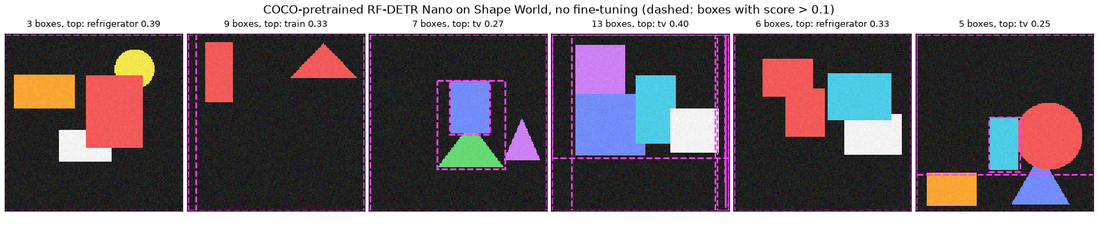
The pink dashed lines are all boxes scoring above 0.1, and each image's title gives the number of boxes and the name and score of the highest-scoring prediction. In the six Shape World test images, most boxes cover the whole image and carry COCO names such as refrigerator and TV.
- At the default threshold of 0.5, almost nothing comes out. 3 detections in 50 images (123 ground-truth objects). The model fairly honestly answers that “there is nothing here I know”.
- Lowering the threshold produces a flood of wrong names. 412 at 0.1 and 2,500 at 0.05 (50 per image). The names given are, from most to least frequent, person 48, tv 46, clock 33, refrigerator 32, apple 24, laptop 22. Given that names of boxy things (TV, refrigerator, laptop) and round things (clock, apple) dominate, the model seems to be fitting unfamiliar shapes into “the most similar thing it knows”.
- The box positions are off too. In test image 0, the highest-scoring prediction calls the whole image (
[0, 0, 192, 192]) a refrigerator (0.39). In Figure 14-2 as well, most pink boxes enclose the whole image or several shapes at once. Occasionally, though, a box fits a single shape closely — meaning that even without knowing the class name, the model senses that “there is some blob here”.
That doesn't make this model useless. Only the labels (the classification head) aren't ours; the backbone, projector, and decoder beneath it already know “how to find objects in an image and draw boxes around them”. Fine-tuning keeps that knowledge, swaps the labels for our classes, and trains a little more. To do that, we first need to put our data into a form the package can read.
Inference-only snapshots
It was omitted from the output above, but the first time you call predict, the package emits this warning once.
[WARNING] rf-detr - Model is not optimized for inference. Latency may be higher than expected. Create predictor = native_model.inference(...) and use predictor.predict(...).
model.predict() runs inference with the same general-purpose PyTorch module used in training. It is convenient but not the fastest route. predictor = model.inference() copies the current weights and returns an inference-only copy with a fixed batch size and resolution (on GPU it uses CUDA graphs, which record the sequence of operations in advance and replay it); from then on you use predictor.predict(image). For half precision, use model.inference(dtype="float16"). How much faster it is gets measured in the latency section.
- optimize_for_inference() is gone
- Older articles and examples often use
model.optimize_for_inference(). Calling it in 1.12.1 raisesAttributeError: 'RFDETRNano' object has no attribute 'optimize_for_inference'. According to the repository's change log (CHANGELOG), the name was changed toinference()in 1.9 and later removed. Also, whereas it used to modify the model itself, the currentinference()leaves the original model untouched and returns a new predictor.
Preparing your data: COCO format
The folder structure the package accepts
train(dataset_dir=…) takes a single folder. The package looks inside and works out the format by itself. According to the documentation and source, it accepts two formats.
| Format | How it is detected | Where the annotations live | Box notation |
| COCO format | | One JSON file per split (train, valid, test) | Pixel |
| YOLO format | | One | Normalized |
If both are present, COCO takes precedence. This chapter uses the COCO format (and the COCO format is also the only one verified by actually running it). The folder looks like this.
ch14_shapes_coco/
├── train/
│   ├── _annotations.coco.json      ← 학습용 주석 (이 이름 그대로여야 한다)
│   ├── 000000.png
│   ├── 000001.png
│   └── …
├── valid/                          ← 검증용. "val" 이 아니라 "valid"
│   ├── _annotations.coco.json
│   └── …
└── test/                           ← 시험용. evaluate(split="test") 가 읽는다
    ├── _annotations.coco.json
    └── …
The roles of the three splits are as seen in Chapter 3. The training set is used to update the weights, the validation set is scored every epoch to choose the best checkpoint, and the test set is looked at only once, at the end. This folder structure is the same as what you get when you download a dataset as “COCO” from the Roboflow service. That's why the default value of train()'s dataset_file argument is named "roboflow".
The three lists in the annotation JSON
_annotations.coco.json is one big dictionary, and the three lists inside it are the core.
| List | One element | Fields |
| | One image | |
| | One class | |
| | One object | |
What feels unfamiliar at first is that images and objects are listed separately and linked by image_id. An image with no objects appears only in images and has no entries at all in annotations. iscrowd marks a region that can't be counted object by object, such as “a crowd of people”. It is usually 0, and according to the documentation, annotations with 1 are not used as training targets.
Converting box coordinates
COCO's bbox is four numbers, [x, y, w, h]. It differs from both of the representations in Chapter 2 (corner format and center format).
- The first two numbers
(x, y)are the box's top-left corner (not the center), and the last two are the width and height - The unit is pixels (not normalized to 0 – 1). The origin is the top-left of the image, and the vertical coordinate increases downward
- In this section only — two units for the same letters w and h
- The width and height in our format and in COCO are both commonly written \(w\) and \(h\), which is confusing. In this section, our normalized format is written \((c_x, c_y, w, h)\) and COCO's pixel values are written \([x^{\text{px}}, y^{\text{px}}, w^{\text{px}}, h^{\text{px}}]\). The image's width and height (in pixels) are uppercase \(W\) and \(H\).
- From normalized (cx, cy, w, h) to COCO [x, y, w, h]
\(x_0 = c_x - \frac{w}{2}, \qquad y_0 = c_y - \frac{h}{2}\)
Chapter 2: the top-left corner is the point half the width to the left of and half the height above the center (still in 0 – 1 units).
\(x^{\text{px}} = x_0 \cdot W = \Big(c_x - \frac{w}{2}\Big) W, \qquad y^{\text{px}} = y_0 \cdot H = \Big(c_y - \frac{h}{2}\Big) H\)
Normalized coordinates are “ratios to the image size”, so multiplying horizontal values by the image width \(W\) and vertical values by the height \(H\) gives pixels.
\([x^{\text{px}},\ y^{\text{px}},\ w^{\text{px}},\ h^{\text{px}}] = \Big[ \Big(c_x - \frac{w}{2}\Big) W,\ \ \Big(c_y - \frac{h}{2}\Big) H,\ \ wW,\ \ hH \Big]\)
The width and height are multiplied by \(W\) and \(H\) for the same reason.
The reverse direction just inverts each formula: add half the width (or height) to the corner to move to the center, then divide by the image size.
\(c_x = \frac{x^{\text{px}} + w^{\text{px}}/2}{W}, \qquad c_y = \frac{y^{\text{px}} + h^{\text{px}}/2}{H}, \qquad w = \frac{w^{\text{px}}}{W}, \qquad h = \frac{h^{\text{px}}}{H}\)
Let's do one by hand. Converting the normalized box \((c_x, c_y, w, h) = (0.5,\ 0.375,\ 0.25,\ 0.5)\) to a COCO box for a 192 × 192 image:
- \(x^{\text{px}} = (0.5 - 0.125) \times 192 = 0.375 \times 192 = 72\)
- \(y^{\text{px}} = (0.375 - 0.25) \times 192 = 0.125 \times 192 = 24\)
- \(w^{\text{px}} = 0.25 \times 192 = 48\), \(\ h^{\text{px}} = 0.5 \times 192 = 96\) →
[72, 24, 48, 96], area \(48 \times 96 = 4608\) - Converting back: \(c_x = (72 + 24)/192 = 0.5\), \(c_y = (24 + 48)/192 = 0.375\) ✓
In a 96 × 96 image, the same box is [36, 12, 24, 48]. Normalized coordinates stay the same when the image size changes, but COCO coordinates depend on the image size. So if you resize images when saving them, you must update the annotations as well.
ch14_make_coco.py · convert
def cxcywh_norm_to_coco(box, width: int, height: int):
    """정규화 (cx, cy, w, h) → COCO bbox [x, y, w, h] (픽셀, (x, y) 는 왼쪽 위 모서리).

    x = (cx − w/2)·W,  y = (cy − h/2)·H,  너비 = w·W,  높이 = h·H
    """
    cx, cy, w, h = (float(v) for v in box)
    return [(cx - w / 2) * width, (cy - h / 2) * height, w * width, h * height]

def coco_to_cxcywh_norm(bbox, width: int, height: int):
    """COCO bbox [x, y, w, h] (픽셀) → 정규화 (cx, cy, w, h). 위 함수의 역변환."""
    x, y, w, h = (float(v) for v in bbox)
    return [(x + w / 2) / width, (y + h / 2) / height, w / width, h / height]
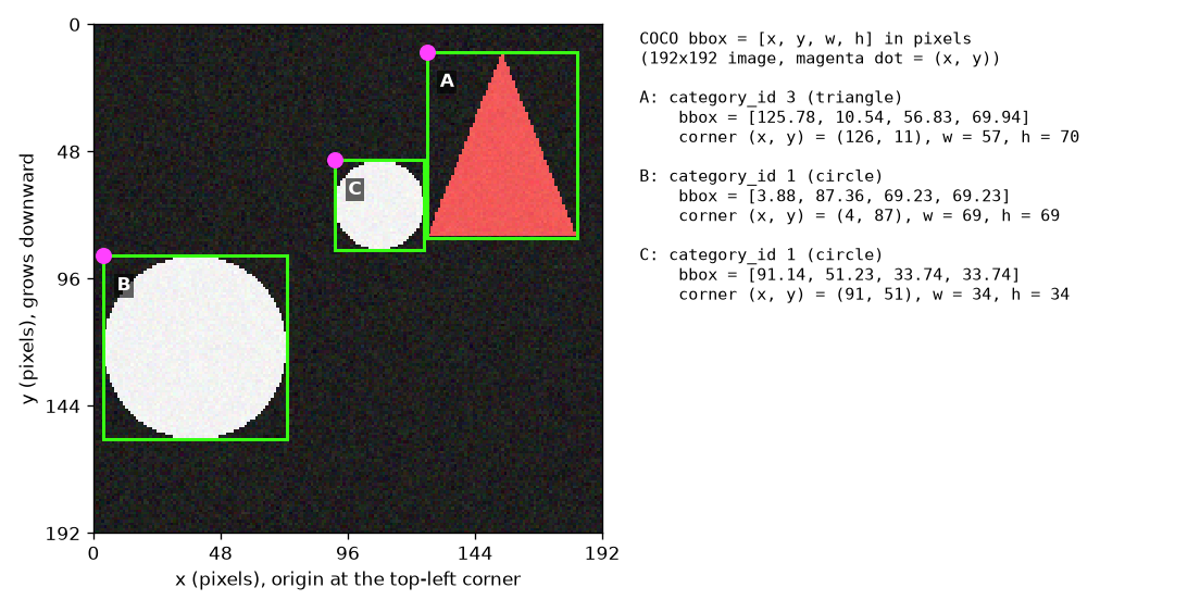
One image from the training set (192×192) and its three annotations. The green rectangles are the boxes, and the pink dots are the first two numbers of bbox, \((x^{\text{px}}, y^{\text{px}})\), that is, the top-left corner. The axis ticks are in pixels, and the vertical axis grows downward.
There are two things to read from Figure 14-3. First, the pink dot is always at the box's top-left (not the center). Second, the last two numbers of each bbox written on the right are not the coordinates of the bottom-right corner but the width and height. Circle B has equal width and height (69.23), and triangle A is taller (69.94) than it is wide (56.83). This is the part most often confused with Chapter 2's corner format \((x_0, y_0, x_1, y_1)\), so take the time to get used to it.
Exporting Shape World
Now we save ShapesDataset as a COCO-format folder. The scenes are generated with the same seeds as in the earlier chapters (training 0, validation 1, test 2), but the images are drawn at 192 pixels instead of 96. As seen in Chapter 0, scenes are described in normalized coordinates, so they can be drawn at any resolution. There are 1,000 training, 200 validation, and 200 test images.
ch14_make_coco.py · export
def export_split(dataset: ShapesDataset, split_dir: str) -> dict:
    """데이터셋 하나를 COCO 형식 폴더 하나로 저장하고, 저장한 주석 사전을 돌려준다.

    COCO 주석 JSON 은 목록 세 개로 이루어진다.
      images:      그림마다 {"id", "file_name", "width", "height"}
      categories:  클래스마다 {"id", "name", "supercategory"} — COCO 의 관례대로 id 를 1 부터 매긴다.
      annotations: 객체마다 {"id", "image_id", "category_id", "bbox", "area", "iscrowd"}
    """
    os.makedirs(split_dir, exist_ok=True)
    size = dataset.size
    images, annotations = [], []
    for image_id, target in enumerate(dataset.targets):
        file_name = f"{image_id:06d}.png"
        pixels = dataset.images[image_id].permute(1, 2, 0).numpy()  # (3, S, S) uint8 → (S, S, 3)
        Image.fromarray(pixels).save(os.path.join(split_dir, file_name))  # PNG: 손실 없이 저장
        images.append({"id": image_id, "file_name": file_name, "width": size, "height": size})
        for box, label in zip(target["boxes"].tolist(), target["labels"].tolist()):
            bbox = cxcywh_norm_to_coco(box, size, size)
            annotations.append({
                "id": len(annotations) + 1,          # 주석 번호 (데이터셋 안에서 유일하면 된다)
                "image_id": image_id,                # 어느 그림의 객체인가
                "category_id": int(label) + 1,       # 우리 클래스 0, 1, 2 → COCO 범주 id 1, 2, 3
                "bbox": [round(v, 2) for v in bbox],  # [x, y, w, h] 픽셀
                "area": round(round(bbox[2], 2) * round(bbox[3], 2), 2),  # 넓이 (여기서는 박스 넓이 w·h)
                "iscrowd": 0,                        # 1 이면 "여럿이 뭉친 영역" — 학습 정답으로 쓰지 않는다
            })
    coco = {
        "info": {"description": "Shape World (RF-DETR tutorial, chapter 14)"},
        "licenses": [],
        "images": images,
        "categories": [{"id": k + 1, "name": name, "supercategory": "shape"} for k, name in enumerate(CLASS_NAMES)],
        "annotations": annotations,
    }
    with open(os.path.join(split_dir, ANNOTATION_FILE), "w", encoding="utf-8") as f:
        json.dump(coco, f)
    return coco
We also write a function that reads the saved folder back into ground truth in our format. It is used later to score the test set with Chapter 3's evaluate_ap. Then we check that the boxes that went through “save → read back” match the originals.
ch14_make_coco.py · load
def load_coco_split(split_dir: str):
    """COCO 형식 폴더를 읽어 (그림 경로 목록, 정답 목록) 을 돌려준다.

    정답은 이 튜토리얼의 형식: {"boxes": (n, 4) 정규화 (cx, cy, w, h), "labels": (n,) 0 부터의 클래스 번호}.
    범주 id 를 작은 것부터 0, 1, 2 … 로 다시 매긴다 — rfdetr 패키지가 학습할 때 하는 일과 같다.
    """
    with open(os.path.join(split_dir, ANNOTATION_FILE), encoding="utf-8") as f:
        coco = json.load(f)
    cat_to_label = {cat_id: k for k, cat_id in enumerate(sorted(c["id"] for c in coco["categories"]))}
    by_image = {image["id"]: [] for image in coco["images"]}
    for ann in coco["annotations"]:
        by_image[ann["image_id"]].append(ann)
    paths, targets = [], []
    for image in coco["images"]:
        anns = by_image[image["id"]]
        boxes = [coco_to_cxcywh_norm(a["bbox"], image["width"], image["height"]) for a in anns]
        paths.append(os.path.join(split_dir, image["file_name"]))
        targets.append({
            "boxes": torch.tensor(boxes, dtype=torch.float32).reshape(-1, 4),
            "labels": torch.tensor([cat_to_label[a["category_id"]] for a in anns], dtype=torch.int64),
        })
    return paths, targets
ch14_make_coco.py · check
def check_roundtrip(dataset: ShapesDataset, split_dir: str) -> float:
    """저장한 폴더를 다시 읽어 원래 정답과 비교한다. 돌려주는 값: 박스 좌표의 최대 차이 (정규화 단위)."""
    paths, targets = load_coco_split(split_dir)
    assert len(paths) == len(dataset)
    worst = 0.0
    for original, loaded in zip(dataset.targets, targets):
        assert original["labels"].tolist() == loaded["labels"].tolist()
        if len(original["boxes"]):
            worst = max(worst, float((original["boxes"] - loaded["boxes"]).abs().max()))
    first = np.asarray(Image.open(paths[0]))  # 그림도 한 장 읽어 픽셀이 그대로인지 본다
    assert np.array_equal(first, dataset.images[0].permute(1, 2, 0).numpy())
    return worst
[1] 손계산 예: 정규화 (cx, cy, w, h) = (0.5, 0.375, 0.25, 0.5)
  96×96 그림 → COCO bbox [x, y, w, h] = [36.0, 12.0, 24.0, 48.0]  (넓이 1152)  → 되돌리면 (0.5, 0.375, 0.25, 0.5)
  192×192 그림 → COCO bbox [x, y, w, h] = [72.0, 24.0, 48.0, 96.0]  (넓이 4608)  → 되돌리면 (0.5, 0.375, 0.25, 0.5)
[2] 도형 세상을 COCO 형식으로 내보내기 → ch14_shapes_coco/  (그림 192×192)
  train: 그림  1000장, 객체  2442개 (circle 807, rectangle 863, triangle 772) | 되읽기 check: 박스 최대 차이 3.8e-05
  valid: 그림   200장, 객체   501개 (circle 169, rectangle 183, triangle 149) | 되읽기 check: 박스 최대 차이 3.8e-05
  test : 그림   200장, 객체   483개 (circle 161, rectangle 163, triangle 159) | 되읽기 check: 박스 최대 차이 3.8e-05
  걸린 시간 15.1초
[3] 주석 파일 들여다보기 (train/_annotations.coco.json)
  images[0]      = {"id": 0, "file_name": "000000.png", "width": 192, "height": 192}
  categories     = [{"id": 1, "name": "circle", "supercategory": "shape"}, {"id": 2, "name": "rectangle", "supercategory": "shape"}, {"id": 3, "name": "triangle", "supercategory": "shape"}]
  annotations[0] = {"id": 1, "image_id": 0, "category_id": 2, "bbox": [6.2, 130.09, 41.38, 29.08], "area": 1203.33, "iscrowd": 0}
  2장 형식의 같은 박스 (cx, cy, w, h) = [0.1401, 0.7533, 0.2155, 0.1515]
  그림 저장: figures/ch14-coco-bbox.png
- Round-trip check. The maximum difference in box coordinates is \(3.8 \times 10^{-5}\) (normalized units). It comes from rounding the annotations to two decimal places in pixels when saving. The rounding error is at most 0.005 pixels per number, so the error of the center \(x^{\text{px}} + w^{\text{px}}/2\) is at most \(0.005 + 0.0025 = 0.0075\) pixels; divided by 192, that is \(3.9 \times 10^{-5}\), consistent with the observed value. It is small enough to ignore.
- Reading one annotation.
annotations[0]is a rectangle (category_id2) in image 0, and itsbboxis[6.2, 130.09, 41.38, 29.08]. Converting back: \(c_x = (6.2 + 41.38/2)/192 = 26.89/192 = 0.1401\), \(c_y = (130.09 + 29.08/2)/192 = 144.63/192 = 0.7533\), \(w = 41.38/192 = 0.2155\), \(h = 29.08/192 = 0.1515\). These match the Chapter 2-format values on the last line. - The three classes are evenly represented (807 circles, 863 rectangles, and 772 triangles in the training set).
Class numbers are reassigned
Our classes are 0, 1, 2, but category_id was deliberately written as 1, 2, 3, following the COCO convention. That's fine. The package (with the default dataset_file="roboflow") lines up the training set's categories in ID order and renumbers them starting from 0.
| | Name | The model's |
| 1 | circle | 0 |
| 2 | rectangle | 1 |
| 3 | triangle | 2 |
In the fine-tuned model, model.class_names was ['circle', 'rectangle', 'triangle'], and predict returned class_id values 0, 1, 2 (see the run output later). The result is the same whether category IDs start from 0 or 1, or have gaps in between. A prediction's class_id is not the JSON category_id but “the position of the category in ID order”. Our load_coco_split numbers classes the same way, so its output can be compared directly with the model's predictions.
Also, you don't need to specify the number of classes. train() counts the categories and rebuilds the classification head at the right size. The warning that appears at that point, and what it means, are covered in the next section.
Resolution and the divisibility constraint
Our images are 192 pixels, while Nano's input is 384. That's no problem. In both training and inference, the package resizes images to the model resolution (along with the annotated boxes). The images in a dataset can even have different sizes.
If you want to change the model resolution, there is one constraint: the side length must be divisible by patch_size × num_windows.
- Why it must be a multiple of patch_size × num_windows
\(N = \frac{S}{P} \quad \text{is an integer}\)
To cut an image side of \(S\) pixels into patches of side \(P\) pixels with no gaps (Chapter 6), \(S\) must be a multiple of \(P\). \(N\) is the number of patches per side.
\(\frac{N}{M} \quad \text{is an integer}\)
Windowed attention divides the \(N \times N\) patch grid into \(M\) equal parts per side, giving \(M \times M\) windows (Chapter 9). For every window to have the same number of patches, \(N\) must be a multiple of \(M\).
\(S = P \cdot M \cdot n \qquad (n = 1, 2, 3, \dots)\)
Combining the two conditions, \(S\) is a multiple of \(P \cdot M\). \(n\) is the number of patches per window side.
For Nano, \(P = 16\) and \(M = 2\), so \(S\) must be a multiple of 32. The default 384 is \(32 \times 12\): the \(24 \times 24\) patches split into 4 windows of \(12 \times 12\). 320, 352, 416, and 448 work; 400 does not (\(400/32 = 12.5\)). If you actually try it, it is rejected like this.
shape=(400, 400) 은 거절된다: shape must have both dimensions divisible by 32 (patch_size=16 * num_windows=2), got (400, 400).
This constraint applies equally to training (train(resolution=…)), inference (predict(shape=…)), and export (export(shape=…)). Segmentation models use a patch size of 12, so the multiple is different (24 for most, 12 for SegNano).
- During training, the resolution changes every batch
- The multi-scale training from Chapter 11 is on by default (
multi_scale="per-batch",expanded_scales=True). Computing Nano's (384) candidate sizes with the installed version's function gives 11 sizes, 224, 256, 288, …, 544: five steps of 32 below and above 384 (0.58 – 1.42 times 384, corresponding to the paper's “0.5 – 1.5 times”). Each batch picks one of these at random and trains at that size. Validation and inference always use 384.
Fine-tuning
A single call to train
Fine-tuning is a single method. Create the model (which loads the pretrained weights) and give train() the dataset folder and an output folder. The training loop hand-written in Chapter 11 — multi-scale training, Group DETR, Hungarian matching, the IA-BCE, L1, and GIoU losses, auxiliary losses, gradient accumulation, gradient clipping, AdamW, EMA, and per-epoch validation — all runs inside this one line. (Internally it is built on PyTorch Lightning.)
ch14_finetune.py · config
# 미세 조정 설정. model.train(**TRAIN_KWARGS) 로 넘긴다. 적지 않은 것은 TrainConfig 의 기본값이다.
TRAIN_KWARGS = dict(
    epochs=5,              # 기본 100. 도형 세상은 쉬워서 몇 에폭이면 충분하다
    batch_size=2,          # 기본 4. 한 번에 GPU 에 올리는 그림 수 — 8GB GPU 를 나눠 쓰느라 작게 잡았다
    grad_accum_steps=4,    # 기본 1. 기울기를 4번 모아 한 번 갱신 → 실효 배치 크기 2 × 4 = 8
    lr=1e-4,               # 기본 1e-4 (디코더 쪽). 백본은 lr_encoder=1.5e-4 에 층별 감쇠 0.8 이 곱해진다
    num_workers=2,         # 기본 2. 데이터 로더 일꾼 수
    seed=0,
    tensorboard=False,     # 기본 True. 이 실습은 metrics.csv 만 읽는다 (wandb · mlflow 는 기본이 False)
    eval_base_model=True,  # 기본 False(EMA 가중치만 검증). EMA 와 일반 가중치를 둘 다 검증해 비교한다
    compact_train_metrics=False,  # 기본 True(보조 손실을 _aux 하나로 합쳐 기록). 층별 손실을 따로 본다
    progress_bar=None,
)
SCRATCH_EPOCHS = 3  # (b) 무작위 초기화는 3 에폭만 돌린다 (GPU 시간을 아끼려고). 그 밖의 설정은 (a) 와 같다
OUT_PRETRAINED = "ch14_out_pretrained"
OUT_SCRATCH = "ch14_out_scratch"
RESULTS_FILE = "ch14_finetune_results.json"
ch14_finetune.py · train
def finetune(output_dir: str, dataset_dir: str, pretrained: bool, retrain: bool, **overrides) -> dict:
    """RF-DETR Nano 를 dataset_dir 로 미세 조정한다. 돌려주는 값: {"minutes": 걸린 시간, "peak_gib": GPU 메모리 최대}.

    학습을 마치면 같은 값을 output_dir/train_info.json 에 적어 두고, 다음에 부르면 학습을 건너뛰고 그것을 읽는다.

    pretrained=True : RFDETRNano() — COCO 까지 학습된 가중치(rf-detr-nano.pth)에서 시작.
    pretrained=False: RFDETRNano(pretrain_weights=None) — 가중치를 읽지 않는다. Nano 는 패치 16 · 위치 임베딩
                      24×24 라 DINOv2 원본(패치 14)도 읽을 수 없어, 백본까지 전부 무작위 초기화로 시작한다.
    """
    from rfdetr import RFDETRNano

    info_path = os.path.join(output_dir, "train_info.json")
    if os.path.exists(os.path.join(output_dir, "checkpoint_best_total.pth")) and os.path.exists(info_path) and not retrain:
        with open(info_path, encoding="utf-8") as f:
            info = json.load(f)
        print(f"  {output_dir}/ 에 학습 결과가 있어 건너뜀 (--retrain 으로 다시 학습).")
        print(f"  그때의 기록: {info['minutes']:.1f}분, GPU 메모리 최대 {info['peak_gib']:.2f} GiB (torch 가 할당한 양)")
        return info
    model = RFDETRNano() if pretrained else RFDETRNano(pretrain_weights=None)
    if torch.cuda.is_available():
        torch.cuda.reset_peak_memory_stats()
    start = time.time()
    # 클래스 수는 주지 않는다: train() 이 train/_annotations.coco.json 의 categories 를 세어
    # 분류 머리를 (클래스 수 + 1) 칸으로 다시 만든다 (이때 머리의 가중치는 새로 초기화된다).
    model.train(dataset_dir=dataset_dir, output_dir=output_dir, **{**TRAIN_KWARGS, **overrides})
    peak = torch.cuda.max_memory_allocated() / 2**30 if torch.cuda.is_available() else float("nan")
    info = {"minutes": round((time.time() - start) / 60, 1), "peak_gib": round(peak, 2)}
    with open(info_path, "w", encoding="utf-8") as f:
        json.dump(info, f)
    print(f"  학습 끝: {info['minutes']:.1f}분, GPU 메모리 최대 {info['peak_gib']:.2f} GiB (torch 가 할당한 양)")
    return info
- Does anything get sent outside?
- The installed version's
TrainConfigdefaults arewandb=False,mlflow=False, andclearml=False, with onlytensorboard=True. TensorBoard just writes files into the output folder and sends nothing anywhere. In other words, unless you turn something on, training logs are not uploaded to any external service. This exercise turns even TensorBoard off withtensorboard=Falseand reads onlymetrics.csv, which is always written. (The only network access is downloading the pretrained weights at the start.)
Main arguments and defaults
train()'s keyword arguments become fields of TrainConfig as is. The defaults below were read from rfdetr/config.py in the installed version (1.12.1). A misspelled name (e.g., epoch=10) is not silently ignored; it raises an error.
| Argument | Default | Meaning | Earlier chapter |
| | (required) | COCO- or YOLO-format dataset folder | This chapter |
| | | Folder where checkpoints and logs are written | |
| | 100 | How many passes to make over the training set | |
| | 4 | Number of images loaded onto the GPU at once. With | |
| | 1 | How many gradients to accumulate before one update | |
| | 1e-4 | Learning rate (projector, heads, etc.). For the decoder, this is multiplied by | |
| | 1.5e-4 | Base learning rate of the backbone (DINOv2). Layer-wise decay is multiplied onto this | |
| | 0.8 | Layer-wise learning rate decay rate | |
| | 0.7 | Per-component (decoder, backbone) learning rate decay rate | This chapter |
| | 1e-4 | Weight decay (AdamW) | |
| | 0.0 | Length of the learning rate warm-up. 0 = no warm-up | |
| | 0.1 | Maximum norm for gradient clipping | |
| | True, 0.993, 100 | Exponential moving average (EMA) of the weights | |
| | "per-batch", True | Multi-scale training that changes the resolution every batch | |
| | 0.0 | Drop path probability | |
| | False | Stop early if validation AP stops improving ( | This chapter |
| | 10 | Save a | |
| | None | Path of the checkpoint ( | This chapter |
| | (model default) | Changes the training resolution. Must be a multiple of | |
| | 2 | Number of data loader workers (processes) | |
| | None | Random seed | |
| | True / False / False | Logging tools | |
| | False | Whether to also score the test set after training finishes |
Things like the loss weights (classification 1, L1 5, GIoU 2), the number of query groups (group_detr=13), and whether IA-BCE is used (ia_bce_loss=True) are not training arguments but part of the model configuration, and are usually left alone. Summarized in one line, the defaults are “learning rate 1e-4, no warm-up, gradients clipped at 0.1, layer-wise decay 0.8, EMA 0.993”, the same as the settings in Appendix A of the paper, seen in Chapter 11. The learning rate schedule also follows the paper's “training without a scheduler”. The installed version's default schedule (lr_scheduler="step") lowers the learning rate to 1/10 only after 100 epochs, and since the default number of epochs is 100, the learning rate stays constant throughout training (it was constant in this experiment's metrics.csv as well).
Effective batch size
With little GPU memory, only a few images fit at once. But if the batch is too small, the gradient is swayed by the particulars of a few images and becomes erratic. Gradient accumulation from Chapter 11 decouples the two: it runs forward and backward passes several times on small batches, summing the gradients, and then updates the weights once. The number of images seen per weight update is called the effective batch size.
\(B_{\text{eff}} = B \times A\)
\(B\) is batch_size (the number of images loaded onto the GPU at once), \(A\) is grad_accum_steps (the number of gradients accumulated), and \(B_{\text{eff}}\) is the effective batch size. With \(N_{\text{train}}\) training images, the number of forward passes and weight updates per epoch are
\(\text{forward passes} = \frac{N_{\text{train}}}{B}, \qquad \text{updates} = \frac{N_{\text{train}}}{B \times A} = \frac{N_{\text{train}}}{B_{\text{eff}}}\)
Plugging in this experiment's values, \(N_{\text{train}} = 1000\), \(B = 2\), and \(A = 4\), so
- The effective batch size is \(B_{\text{eff}} = 2 \times 4 = 8\)
- Each epoch has \(1000 / 2 = 500\) forward passes and \(1000 / 8 = 125\) weight updates
- Five epochs make \(5 \times 125 = 625\) updates in total. In the actual
metrics.csv, thestepon the last row is 624 (counting from 0, so it is the 625th).
Memory depends only on \(B\). With batch_size=2, this training used at most 1.61 GiB of GPU memory. Building the same effective batch of 8 with batch_size=8, grad_accum_steps=1 gives (nearly) the same update, but needs several times as much memory.
- How to choose the batch
-
- The documentation recommends “first raising
batch_sizeas far as the GPU allows, and raisinggrad_accum_stepsonly if that is still not enough”. Accumulation saves memory, not time. -
batch_size="auto"(CUDA only) probes the GPU to find a batch that fits, and sets the accumulation count so that the effective batch reaches 16 (the default ofauto_batch_target_effective). This chapter didn't use it because the GPU was shared with other jobs. - RF-DETR tolerates accumulation well thanks to a choice seen in Chapter 10: the projector's batch normalization was replaced with layer normalization, so the normalization statistics don't fluctuate even with a batch of only two images.
- The documentation recommends “first raising
Different learning rates for different components
We said “learning rate 1e-4”, but not every weight learns at that rate. Reading the installed version's training/param_groups.py and models/backbone/backbone.py shows that each component's rate is set as follows. \(\eta\) is lr, \(\eta_{\text{enc}}\) is lr_encoder, \(\rho\) is lr_component_decay (0.7), \(\lambda\) is lr_vit_layer_decay (0.8), \(L\) is the number of blocks used in the backbone plus 1 (13 for Nano), and \(j\) is the backbone block number (0 – 11).
| Component | Learning rate | With Nano defaults |
| Projector, classification and box heads, query embeddings, etc. | \(\eta\) | \(1.0 \times 10^{-4}\) |
| Decoder | \(\eta \cdot \rho\) | \(10^{-4} \times 0.7 = 7.0 \times 10^{-5}\) |
| Backbone block \(j\) | \(\eta_{\text{enc}} \cdot \lambda^{\,L - j} \cdot \rho^2\) | Block 11: \(4.70 \times 10^{-5}\) … Block 0: \(4.04 \times 10^{-6}\) |
| Backbone patch and positional embeddings | \(\eta_{\text{enc}} \cdot \lambda^{\,L + 1} \cdot \rho^2\) | \(3.23 \times 10^{-6}\) |
- Worked by hand — learning rates of the top backbone block and the bottom embeddings
\(\eta_{\text{enc}} \cdot \rho^2 = 1.5 \times 10^{-4} \times 0.7^2 = 1.5 \times 10^{-4} \times 0.49 = 7.35 \times 10^{-5}\)
This is the factor common to the whole backbone. The component decay of 0.7 is applied once to the decoder and twice to the backbone (the farther from the output, the smaller).
\(\text{block } 11:\quad 7.35 \times 10^{-5} \times 0.8^{\,13 - 11} = 7.35 \times 10^{-5} \times 0.64 = 4.70 \times 10^{-5}\)
The last block (\(j = 11\)) has the decay applied only twice.
\(\text{block } 0:\quad 7.35 \times 10^{-5} \times 0.8^{13} = 7.35 \times 10^{-5} \times 0.05498 = 4.04 \times 10^{-6}\)
The first block has it applied 13 times. \(0.8^{13} = 0.05498\) (\(0.8^2 = 0.64\), \(0.8^4 = 0.4096\), \(0.8^8 = 0.16777\), \(0.8^{13} = 0.8^8 \cdot 0.8^4 \cdot 0.8 = 0.05498\)).
\(\text{embeddings}:\quad 7.35 \times 10^{-5} \times 0.8^{14} = 7.35 \times 10^{-5} \times 0.04398 = 3.23 \times 10^{-6}\)
The patch and positional embeddings get it once more and have the smallest rate, about 1/31 of the head's (1e-4).
This hand calculation matches the actual training log. metrics.csv records the largest and smallest learning rates among the optimizer's parameter groups, and in this run they were lr_max 0.0001 and lr_min 3.233e-06 (see the run output later). These are the top and bottom rows of the table above.
Why do this? It is exactly the layer-wise learning rate decay from Chapter 11. The lower layers of the backbone hold general knowledge such as “edges, textures, and shapes” that DINOv2 learned from over 100 million images, so it is safer to change them only slightly, while the newly built head has to change a lot to fit our data. It is a mechanism for protecting pretrained knowledge during fine-tuning.
The head reinitialization warning
When training starts, a warning like this scrolls past in the log.
[WARNING] rf-detr - Checkpoint has 90 classes but model is configured for 3. The detection head will be re-initialized to 3 classes.
It is not an error but a notice that what you wanted has happened. The classification head of the pretrained weights has 91 slots for COCO, while our data has 3 classes. The package counts the dataset's categories, sets num_classes to 3, and builds a new classification head with number of classes + 1 = 4 slots (reinitialize_detection_head). Printing the head of the fine-tuned model shows Linear(in_features=256, out_features=4, bias=True) (see the run output later).
- What “re-initialized” actually means. From the warning alone you would expect the new head to be filled with random values, but the installed version's source (
_resize_linear) doesn't do that. It takes the first 4 of the original head's 91 rows and uses them as the new head (if there are more than 91 classes, it instead repeats rows and concatenates them). Checking directly, the classification head weights ofRFDETRNano(num_classes=3)differed from rows 0 – 3 of the COCO model's head by exactly 0, and the biases were −4.4 to −4.7, close to the “prior probability 0.01” initialization value \(-\log(0.99/0.01) = -4.595\) seen in Chapter 10. In other words, our “circle” starts from COCO's unused slot 0, “rectangle” from the person slot, and “triangle” from the bicycle slot. These values have nothing to do with shapes, so in practice it is still a head that has to be learned anew. Everything below the head (backbone, projector, decoder, box head) keeps the pretrained weights. - The one extra slot (the last one) is unused. Since no ground truth ever points to it, its score approaches 0 as training proceeds. However, if you remove the threshold entirely, as in
predict(threshold=0.0), predictions for that slot (class_id= 3) come out as well. That is whydetections_to_predictionhas a line that filters them out withnum_classes. - If you pass the number of classes directly when creating the model, as in
RFDETRNano(num_classes=5), your value is kept even if it differs from the dataset, and only a warning is issued (_align_num_classes_from_datasetin the source). Unless you have a specific reason, don't pass it; let the package count.
Loss names in the training log
At the end of every epoch, the training losses and validation metrics are appended as one row to metrics.csv in the output folder. If you can read the column names, you can see which part of the model is learning and how. With the default setting (compact_train_metrics=True), the auxiliary losses are logged merged into one, as in loss_ce_aux, so this exercise turned that off to get them per layer.
| Column name (after | What it is | Weight | Earlier chapter |
| | Classification loss. The name says ce (cross-entropy), but it is actually IA-BCE ( | 1 | |
| | L1 distance between matched predicted boxes and ground-truth boxes (normalized coordinates) | 5 | |
| | \(1 - \operatorname{GIoU}\) | 2 | |
| | Auxiliary losses: the same losses applied to the output of decoder layer 0 (the first layer). Nano's decoder has 2 layers, so there is only | Same | |
| | Losses on the proposals made from the encoder (projector) output in two-stage query selection. These are predictions before the decoder | Same | |
| | The sum of all 9 terms above, each multiplied by its weight. This single number is what gets backpropagated | ||
| | Reference metrics (not part of the loss). The class error rate (%) of matched queries, and the absolute value of “number of queries scoring above 0.5 − number of ground-truth objects” | – | |
| | Learning rates (previous section) | – |
Written as a formula, the total loss is as follows. \(\ell\) is an index for where the loss is applied (the last decoder layer, decoder layer 0, the encoder proposals).
\(\mathcal{L} = \sum_{\ell \,\in\, \{\text{last},\ 0,\ \text{enc}\}} \Big( 1 \cdot \mathcal{L}^{(\ell)}_{\text{ce}} + 5 \cdot \mathcal{L}^{(\ell)}_{\text{bbox}} + 2 \cdot \mathcal{L}^{(\ell)}_{\text{giou}} \Big)\)
\(\mathcal{L}^{(\ell)}_{\text{ce}}\), \(\mathcal{L}^{(\ell)}_{\text{bbox}}\), and \(\mathcal{L}^{(\ell)}_{\text{giou}}\) are the classification, L1, and GIoU losses at position \(\ell\). You can check this formula against the logged values. Plugging in the first epoch's values:
- Classification: \(0.4325 + 0.7244 + 0.6895 = 1.8464\)
- L1: \(5 \times (0.0181 + 0.0198 + 0.0558) = 5 \times 0.0937 = 0.4685\)
- GIoU: \(2 \times (0.0515 + 0.0556 + 0.1499) = 2 \times 0.2570 = 0.5140\)
- Sum: \(1.8464 + 0.4685 + 0.5140 = 2.8289\). The logged
lossis 2.8288 (the difference in the fourth decimal place is due to rounding). ✓
Just setting the losses at the three positions side by side reveals the architecture. In the same epoch, the classification loss is smaller at the last layer (0.4325) than at the encoder proposals (0.6895) and decoder layer 0 (0.7244), and the box loss of the encoder proposals (0.0558) is about three times that of the decoder layers (0.0198, 0.0181). It is exactly the picture from Chapter 8 and Chapter 10: the decoder refines the encoder's rough proposals layer by layer.
Results by epoch
Now for the results of the actual run. Starting from the pretrained weights, the model was trained for 5 epochs on 1,000 Shape World images. Below, metrics.csv is summarized in one line per epoch (the long log the package prints to the screen is omitted). This output comes from a second run made to redraw the figures after training, so it shows a “skipped” line. On the first run, training happens at that point and 학습 끝: 18.2분, GPU 메모리 최대 1.61 GiB (training finished: 18.2 minutes, peak GPU memory 1.61 GiB) is printed.
ch14_finetune.py · read-metrics
def read_metrics(output_dir: str) -> list[dict]:
    """output_dir/metrics.csv 를 에폭별 사전의 목록으로 읽는다.

    Lightning 의 CSV 기록은 에폭마다 두 줄(검증 지표 줄, 학습 손실 줄)을 쓰고 빈 칸은 비워 둔다.
    같은 에폭의 두 줄을 하나로 합친다. 열 이름은 "train/loss_ce", "val/mAP_50_95" 같은 식이다.
    """
    epochs: dict[int, dict] = {}
    with open(os.path.join(output_dir, "metrics.csv"), encoding="utf-8") as f:
        for row in csv.DictReader(f):
            merged = epochs.setdefault(int(row["epoch"]), {"epoch": int(row["epoch"])})
            for key, value in row.items():
                if key not in ("epoch", "step") and value not in ("", None):
                    merged[key] = float(value)
    return [epochs[k] for k in sorted(epochs)]
[2] 미세 조정 (a) 사전 학습 가중치에서 시작 → ch14_out_pretrained/
  설정: epochs=5, batch_size=2, grad_accum_steps=4, lr=0.0001, num_workers=2, seed=0, tensorboard=False, eval_base_model=True, compact_train_metrics=False, progress_bar=None
  ch14_out_pretrained/ 에 학습 결과가 있어 건너뜀 (--retrain 으로 다시 학습).
  그때의 기록: 18.2분, GPU 메모리 최대 1.61 GiB (torch 가 할당한 양)
  metrics.csv 의 손실 열: loss, loss_bbox, loss_bbox_0, loss_bbox_enc, loss_ce, loss_ce_0, loss_ce_enc, loss_giou, loss_giou_0, loss_giou_enc
  에폭 | loss    | loss_ce loss_bbox loss_giou | loss_ce_0 loss_ce_enc | val AP(일반) AP(EMA) AP50(EMA)
     1 |   2.829 |   0.433    0.0181    0.0515 |     0.724       0.689 |      0.9417  0.9476    0.9998
     2 |   2.072 |   0.243    0.0177    0.0524 |     0.464       0.440 |      0.9772  0.9792    1.0000
     3 |   1.530 |   0.189    0.0138    0.0419 |     0.349       0.328 |      0.9754  0.9816    0.9999
     4 |   1.425 |   0.182    0.0136    0.0409 |     0.278       0.321 |      0.9808  0.9832    0.9999
     5 |   1.513 |   0.178    0.0131    0.0394 |     0.348       0.327 |      0.9822  0.9839    0.9999
  첫 에폭의 손실 항목: loss 2.8288, loss_bbox 0.0181, loss_bbox_0 0.0198, loss_bbox_enc 0.0558, loss_ce 0.4325, loss_ce_0 0.7244, loss_ce_enc 0.6895, loss_giou 0.0515, loss_giou_0 0.0556, loss_giou_enc 0.1499
  cardinality_error (에폭별): 25.09, 28.98, 29.23, 29.03, 29.19 | lr_max 0.0001 lr_min 3.233e-06
  check: 1·Σloss_ce + 5·Σloss_bbox + 2·Σloss_giou = 1.513  vs  기록된 loss = 1.513
  출력 폴더: checkpoint_best_ema.pth (121 MB), checkpoint_best_regular.pth (242 MB), checkpoint_best_total.pth (121 MB), last.ckpt (483 MB), last_ema.pth (121 MB), metrics.csv, train_info.json, training_config.json
- It is essentially done after the first epoch. After 125 weight updates, validation AP is 0.9417 (regular weights) and 0.9476 (EMA weights), and AP50 is 0.9998. This is the same model that called shapes refrigerators before fine-tuning. After 5 epochs it reaches 0.9822 / 0.9839.
- AP50 is pinned at 1, while AP rises slowly around 0.98. As seen in Chapter 3, AP@[.50:.95] averages over IoU thresholds up to 0.95. “Roughly right boxes” (IoU 0.5) are almost all correct from the first epoch, and the remaining difference comes from “whether the boxes fit tightly enough to exceed IoU 0.9”. The gradual decrease in the box losses (
loss_bbox0.0181 → 0.0131,loss_giou0.0515 → 0.0394) is that process. - The EMA weights are slightly better every time (0.9476 vs. 0.9417, 0.9792 vs. 0.9772, …, 0.9839 vs. 0.9822). The difference is small, 0.002 – 0.006, but it points the same way in all five epochs. As seen in Chapter 11, averaging the weights over many steps smooths out the jitter of individual steps. The regular weights' AP dipped once at epoch 3 (0.9772 → 0.9754), but the EMA's never went down.
- The total loss actually rose from epoch 4 to epoch 5 (1.425 → 1.513), because the auxiliary loss
loss_ce_0jumped from 0.278 to 0.348. Yet validation AP kept rising. The training loss is measured under multi-scale training and augmentation, with the resolution changing every batch, so it is common for the average over one epoch to go up and down a little. The criterion for choosing a model is validation AP, not training loss. - Why cardinality_error is around 29. It isn't shown in the output, but this column of
metrics.csvstays at 29.0 – 29.2 from epoch 2 on. This is not a malfunction. During training, the Group DETR of Chapter 9 runs 13 query groups together, and each group makes one prediction per object. An image has \(2442/1000 = 2.44\) objects on average, so about \(13 \times 2.44\) queries score above 0.5, and the difference from the ground-truth count is \(12 \times 2.44 = 29.3\). This matches the observed value. In effect, a single number in the log confirms that Group DETR is actually running.
The power of pretraining
Is it this easy because of the model architecture or because of pretraining? There is one way to tell: train with exactly the same settings, minus only the pretrained weights. Creating the model with RFDETRNano(pretrain_weights=None) loads no weight file. The package then reports “Using patch size 16 instead of 14, which means we're not loading DINOv2 backbone weights and the backbone starts from random initialization”. Because Nano's patch size is 16, it can't load the original DINOv2 (patch 14) as is either, so it starts with everything from the backbone to the head randomly initialized. To save GPU time, this run was only 3 epochs. Apart from the number of epochs, all settings are the same and the learning rate is constant throughout, so comparing epoch for epoch is fair.
[3] 미세 조정 (b) 무작위 초기화에서 시작 (epochs=3, 나머지 설정은 같음) → ch14_out_scratch/
  ch14_out_scratch/ 에 학습 결과가 있어 건너뜀 (--retrain 으로 다시 학습).
  그때의 기록: 8.5분, GPU 메모리 최대 1.61 GiB (torch 가 할당한 양)
  metrics.csv 의 손실 열: loss, loss_bbox, loss_bbox_0, loss_bbox_enc, loss_ce, loss_ce_0, loss_ce_enc, loss_giou, loss_giou_0, loss_giou_enc
  에폭 | loss    | loss_ce loss_bbox loss_giou | loss_ce_0 loss_ce_enc | val AP(일반) AP(EMA) AP50(EMA)
     1 |   9.972 |   0.776    0.2797    0.5711 |     0.760       0.733 |      0.3384  0.3244    0.5972
     2 |   6.901 |   0.848    0.1534    0.3076 |     0.875       1.018 |      0.6059  0.6342    0.8311
     3 |   5.782 |   0.758    0.1173    0.2154 |     0.804       0.988 |      0.7532  0.7749    0.8902
  첫 에폭의 손실 항목: loss 9.9724, loss_bbox 0.2797, loss_bbox_0 0.2865, loss_bbox_enc 0.2747, loss_ce 0.7758, loss_ce_0 0.7599, loss_ce_enc 0.7331, loss_giou 0.5711, loss_giou_0 0.5793, loss_giou_enc 0.5989
  cardinality_error (에폭별): 2.52, 9.58, 18.62 | lr_max 0.0001 lr_min 3.233e-06
  check: 1·Σloss_ce + 5·Σloss_bbox + 2·Σloss_giou = 5.782  vs  기록된 loss = 5.782
- Figure: Figure 14-4. Fine-tuning curves
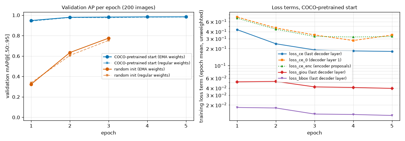
The left panel shows validation AP@[.50:.95] per epoch. Blue starts from the pretrained weights and orange from random initialization; solid lines are the EMA weights and dashed lines the regular weights. The right panel shows the per-term loss curves (before weighting, log-scale vertical axis) of the run started from the pretrained weights.
Here are the two runs side by side, epoch for epoch (validation AP@[.50:.95], EMA weights).
| Epoch (updates) | (a) Started from pretraining | (b) Started from random initialization | AP50 of (b) |
| 1 (125) | 0.9476 | 0.3244 | 0.5972 |
| 2 (250) | 0.9792 | 0.6342 | 0.8311 |
| 3 (375) | 0.9816 | 0.7749 | 0.8902 |
| 5 (625) | 0.9839 | (not run) |
- One epoch of the pretrained model is far ahead of three epochs from random initialization (0.948 vs. 0.775). In the left panel of Figure 14-4, the blue line hugs the ceiling from the start while the orange line is still climbing up from the floor.
- The gap is largest in the boxes. In the first epoch,
loss_bboxis 0.0181 for (a) vs. 0.2797 for (b), a factor of 15, andloss_giouis 0.0515 vs. 0.5711, a factor of 11. (a) starts out already knowing “how to put a box around an object” and only has to learn the new labels, while (b) first has to learn what an edge is. The gap between (b)'s AP50 (0.89) and AP (0.77) being much wider than (a)'s tells the same story — it finds the objects but can't box them tightly. - To be fair, (b) also climbs quite far. After 3 epochs, 375 weight updates, it is at 0.77 and still rising. Running it longer would narrow the gap further. That's because Shape World is such easy data (plain background, distinct colors, three classes). With complex data such as photos, it is a different story. The LW-DETR paper reported that Objects365 pretraining adds +8.7 mAP on COCO, and the RF-DETR paper switched the backbone to DINOv2 for the sake of “accuracy on small datasets” (Chapter 6, Chapter 10). What this experiment shows is not the magnitude but the direction: with the same data and the same time, starting from pretraining gets you much further.
- EMA doesn't always win. In (b)'s first epoch, the EMA weights (0.3244) are worse than the regular weights (0.3384). While the model is improving quickly, “the average of past weights” lags behind the current weights. In epochs 2 and 3, EMA is ahead again (0.6342 vs. 0.6059, 0.7749 vs. 0.7532). This is why the package picks the better of the two when creating
checkpoint_best_total.pth. - (b)'s classification loss
loss_cebarely decreases, 0.776 → 0.848 → 0.758, yet AP rises. The IA-BCE of Chapter 9 ties the classification target to the IoU of the predicted box, so as the boxes improve, the target rises with them. This shows again that it is hard to judge from a single loss value whether training is going well. - Training took 18.2 minutes for (a)'s 5 epochs and 8.5 minutes for (b)'s 3 epochs, and both peaked at 1.61 GiB of GPU memory. The GPU was being shared with several other training jobs at the time, so treat the times only as a rough reference. With the GPU to yourself it is faster.
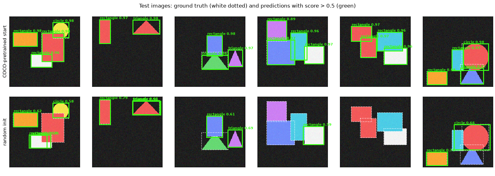
Six test images (the same images as in Figure 14-2). White dashed lines are the ground truth, and green solid lines are predictions scoring above 0.5. The top row is the model started from the pretrained weights, and the bottom row the model started from random initialization.
- Top row (started from pretraining). Every shape in all six images gets exactly one box, drawn almost on top of the ground truth (white dashed lines), with scores of 0.89 – 0.98. Overlapping shapes (fourth and fifth images) are also detected separately. The model that answered refrigerator and TV for these same images in Figure 14-2 got this far with fine-tuning on 1,000 images for 18 minutes.
- Bottom row (random initialization). Few predictions score above 0.5 (none at all in the fifth image), and those that do score low, between 0.5 and 0.8. The white rectangle in the first image and the triangle in the second image each get two overlapping boxes. The model hasn't yet fully learned the “one prediction per object” rule that Hungarian matching teaches (Chapter 7). In the sixth image, the circle's box spreads wide toward the neighboring rectangle.
- The bottom row's model still has a test AP of 0.77 (next section). AP looks only at the order of the scores, so it can be high even when scores are low overall. In real use, cutting at a threshold of 0.5, the model misses a lot, as the figure shows. This is why you should look at both the metrics and the results with your own eyes.
The output folder and checkpoints
When training finishes, several files remain in output_dir. A file that stores the weights during or at the end of training is called a checkpoint. The table below summarizes the files listed in the 출력 폴더 (output folder) line of the output above, after opening each of them.
| File | Size | Contents | Use |
| | 121 MB | The weights with the best validation AP: the better of regular and EMA (EMA this time) + model config and class names | For inference and export. Usually this is all you need |
| | 121 MB | EMA weights from the epoch where the EMA weights had the best validation AP | Ingredient of the file above |
| | 242 MB | Regular weights from the epoch where the regular weights had the best validation AP (large because it also contains an EMA copy) | Ingredient of the file above. Created only when |
| | 483 MB | Regular weights (121) + EMA weights (121) + optimizer state (241) from the last epoch | For resuming training |
| | 121 MB | EMA weights from the last epoch | |
| | Per-epoch losses and validation metrics | Plotting training curves | |
| | All the settings and class names of this training run | Reproducibility and record-keeping |
- What the sizes tell you. One set of weights is 121 MB (about 30.15 million parameters × 4 bytes).
last.ckptis four times that because AdamW remembers two values per parameter (the moving averages of the gradient and of the squared gradient, Chapter 4). The optimizer state is twice the size of the weights (241 MB). - After training, load the result with
rfdetr.from_checkpoint("…/checkpoint_best_total.pth"). The checkpoint records the model type, so it picks the right class (RFDETRNano) by itself and restores the class names as well. You can also callpredictright away on themodelobject you calledtrain()on, but to use the model again in another program or on another day, this is the standard way. -
checkpoint_<epoch>.ckptis saved everycheckpoint_interval(default 10) epochs. This 5-epoch run doesn't have one. -
train_info.jsonis written not by the package but by this exercise's code, to record the time and memory used.
ch14_finetune.py · load
def load_finetuned(output_dir: str = OUT_PRETRAINED):
    """학습이 남긴 checkpoint_best_total.pth 를 읽어 추론할 수 있는 모델을 돌려준다.

    rfdetr.from_checkpoint 는 체크포인트에 적힌 모델 종류 · 해상도 · 클래스 이름을 읽어 알맞은 클래스(RFDETRNano)를
    스스로 고른다. 검증 AP 가 가장 좋았던 가중치(일반과 EMA 가운데 나은 쪽)가 들어 있다.
    """
    import rfdetr

    return rfdetr.from_checkpoint(os.path.join(output_dir, "checkpoint_best_total.pth"))
How the “EMA weights” are produced can also be checked in the installed version's source. At every weight update,
\(\theta_{\text{EMA}} \leftarrow d_t\, \theta_{\text{EMA}} + (1 - d_t)\, \theta, \qquad d_t = d \cdot \big(1 - e^{-t/\tau_{\text{EMA}}}\big)\)
\(\theta\) is the current (regular) weights, \(\theta_{\text{EMA}}\) the EMA weights, \(t\) the number of updates so far, \(d\) is ema_decay (0.993), \(\tau_{\text{EMA}}\) is ema_tau (100), and \(d_t\) is the effective decay rate at the \(t\)-th update. It is the EMA from Chapter 11 with a correction that “makes it follow quickly at first”. At \(t = 100\), \(d_t = 0.993 \times (1 - e^{-1}) = 0.993 \times 0.632 = 0.628\); at \(t = 625\), the end of this experiment, \(d_t = 0.993 \times (1 - e^{-6.25}) = 0.993 \times 0.998 = 0.991\). As \(d_t\) approaches 0.993, the EMA becomes roughly the average of the weights over the last \(1/(1 - 0.993) \approx 143\) updates, a little longer than one epoch (125 updates) in this experiment.
Early stopping and resuming training
If you set a generous number of epochs, at some point validation AP stops rising. Stopping training at that point to save time is called early stopping. In the installed version, you enable it with train(…, early_stopping=True) (it is off by default). According to the documentation, training stops when validation AP (val/mAP_50_95 for detection) fails to improve by more than early_stopping_min_delta (default 0.001) for early_stopping_patience (default 10) epochs. A 5-epoch run like this experiment had no use for it, so it wasn't tried. Whether or not you use early stopping, checkpoint_best_total.pth keeps the weights with the best validation AP, so there is no risk of ending up with “a model that got worse from training too long”.
If training was interrupted, or you want to run more epochs, pass last.ckpt to resume.
model = RFDETRNano()
model.train(dataset_dir="ch14_shapes_coco", output_dir="ch14_out_pretrained",
            epochs=8,                                   # 전체 에폭 수 (이미 돈 5 에폭 포함)
            resume="ch14_out_pretrained/last.ckpt",     # 가중치 · 옵티마이저 상태 · 에폭 번호를 이어받는다
            batch_size=2, grad_accum_steps=4)
-
epochsis not “the number of additional epochs” but the total number of epochs. This was checked with a small dataset (60 images): after training withepochs=1, calling again in the same output folder withresume=…/last.ckpt, epochs=2ran only the second epoch, andmetrics.csvrecorded epoch 0 (step 14) and epoch 1 (step 29) in sequence. - You can resume from
last.ckpt(andcheckpoint_<epoch>.ckpt), which include the optimizer state. According to the documentation, the lightweight.pthfiles have no optimizer state, so resuming from them carries over only the weights. - Calling
train()again, withoutresume, on amodelthat has finished training does not continue training. According to the source, it starts over from the original pretrained weights and issues a warning saying so.
Evaluation
The package's evaluate
The validation set's AP has already been used to choose the best checkpoint, so the final grade is given on the test set, which the model has never seen (Chapter 3). In the package this is one line, model.evaluate(dataset_dir=…, split="test"), which returns a dictionary of metrics.
| Returned key | Meaning | Name in Chapter 3 |
| | AP averaged over the IoU thresholds 0.50, 0.55, …, 0.95 and then over the classes. COCO's headline metric | AP (= AP@[.50:.95], mAP) |
| | AP using only the IoU threshold 0.5 | AP50 |
| | AP using only the IoU threshold 0.75 | AP75 |
| | Mean recall when using up to 500 predictions per image ( | Mean of recall |
| | F1, precision, and recall at the point with the best F1, found by sweeping the score threshold over a range of values | Precision and recall |
| | Loss on the test set |
It is called mAP, but the definition is the same as what was computed by hand in Chapter 3: for each class, sort the predictions by score to draw the precision–recall curve, average the interpolated precision at 101 recall points, and average that over the 10 IoU thresholds and over the classes. The computation is handled by a scoring library that gives the same results as the official COCO scorer (pycocotools).
Checking against the Chapter 3 scorer
Rather than simply trusting the numbers the package reports, we score the same model's predictions directly with our own evaluate_ap and compare. We get all predictions per image with predict(threshold=0.0), convert them to the Chapter 2 format (detections_to_prediction), and feed them in along with the ground truth read by load_coco_split.
ch14_finetune.py · evaluate
def evaluate_both(model, dataset_dir: str, test_paths, test_targets) -> dict:
    """같은 모델 · 같은 시험 세트를 (가) 패키지의 evaluate() 와 (나) 3장의 evaluate_ap 로 채점한다."""
    # (가) 패키지: COCO 방식 채점기로 mAP@[.50:.95], [email protected], [email protected], mAR 등을 돌려준다.
    package = model.evaluate(dataset_dir=dataset_dir, split="test", batch_size=2, num_workers=2, progress_bar=None)
    # (나) 우리 것: predict 로 예측을 모두 받아(문턱값 0 → 그림마다 num_select 개) 직접 채점.
    predictions = predict_all(model, test_paths, threshold=0.0, num_classes=NUM_CLASSES)
    ours = evaluate_ap(predictions, test_targets, NUM_CLASSES)                    # 그림당 상위 100개 (3장 기본값)
    ours_500 = evaluate_ap(predictions, test_targets, NUM_CLASSES, max_dets=500)  # 패키지처럼 500개까지
    return {"package": package, "ours": ours, "ours_500": ours_500, "predictions": predictions}
[4] 시험 세트 채점: 패키지의 evaluate() 와 3장의 evaluate_ap
  from_checkpoint → RFDETRNano, class_names=['circle', 'rectangle', 'triangle'], 분류 머리 Linear(in_features=256, out_features=4, bias=True)
  (pretrained) 패키지 evaluate(): mAP50:95 0.9828, mAP50 1.0000, mAP75 0.9900, mAR 0.9864
  (pretrained) 우리 evaluate_ap : AP      0.9830, AP50  1.0000, AP75  0.9900  | max_dets=500 이면 AP 0.9830  | 클래스별 AP circle 0.989, rectangle 0.996, triangle 0.965
  예측 예 (시험 그림 0, 점수 상위 4개 / 돌려받은 277개):
    rectangle 점수 0.980  (cx, cy, w, h) = [0.225, 0.326, 0.34, 0.193]
    rectangle 점수 0.977  (cx, cy, w, h) = [0.618, 0.44, 0.315, 0.408]
    circle    점수 0.975  (cx, cy, w, h) = [0.732, 0.194, 0.225, 0.215]
    rectangle 점수 0.962  (cx, cy, w, h) = [0.456, 0.633, 0.296, 0.183]
    정답: ['circle', 'rectangle', 'rectangle', 'rectangle'] [[0.731, 0.2, 0.224, 0.224], [0.226, 0.327, 0.344, 0.193], [0.455, 0.632, 0.297, 0.182], [0.618, 0.44, 0.317, 0.411]]
  (scratch) 패키지 evaluate(): mAP50:95 0.7722, mAP50 0.8827, mAP75 0.8582, mAR 0.9132
  (scratch) 우리 evaluate_ap : AP      0.7738, AP50  0.8834, AP75  0.8569  | max_dets=500 이면 AP 0.7738  | 클래스별 AP circle 0.814, rectangle 0.752, triangle 0.754
| Model | Scorer | AP50:95 | AP50 | AP75 |
| (a) Started from pretraining | Package | 0.9828 | 1.0000 | 0.9900 |
| Our | 0.9830 | 1.0000 | 0.9900 | |
| (b) Random initialization | Package | 0.7722 | 0.8827 | 0.8582 |
| Our | 0.7738 | 0.8834 | 0.8569 |
- The two scorers agree. The difference is 0.0002 for (a) and 0.0016 for (b). This means the scorer built by hand in Chapter 3 measures the same thing as the real package's scoring. The test-set AP (0.983) is also almost the same as the validation-set AP (0.984), so the checkpoint chosen on the validation set held up on images it had never seen.
- Why they aren't identical. The cause appears to be not the scoring rules but slight differences in the predictions being scored.
evaluate()runs the forward pass through the same path as training, and, as the log lineUsing bfloat16 Automatic Mixed Precision (AMP)indicates, it computes in 16-bit mixed precision. Our predictions were computed in FP32 bypredict(). When box coordinates differ in some decimal place, a few predictions end up just above or just below an IoU threshold (especially 0.90 and 0.95), and the last digit of AP moves. That the difference is larger for (b), whose boxes are less accurate, is consistent with this explanation. (The explanation was not verified with a separate experiment.) - The limit on predictions per image made no difference. The package scores up to 500 predictions per image (
eval_max_dets) and Chapter 3's default up to 100, but changing our scorer to 500 gave the same AP (0.9830). Images have at most 4 objects, so there are no useful predictions outside the top 100. - By class, (a) scores rectangle 0.996, circle 0.989, and triangle 0.965. With AP50 at 1.0, almost nothing is missed or misnamed; the differences come from how tightly the boxes fit at high IoU thresholds. The triangle boxes fit slightly less tightly.
- Looking at the predictions directly, in test image 0 the top four predictions by score correspond one-to-one with the four ground-truth objects. For example, the prediction
(0.225, 0.326, 0.34, 0.193)and the ground truth(0.226, 0.327, 0.344, 0.193)agree to within 0.004. 277 predictions were returned: the 300 fromnum_selectminus 23 predictions for the unused fourth slot that were filtered out.
Trying different inference settings
Even a trained model gives different results depending on how you use it. Keeping the weights fixed, we vary three inference settings. All are measured with fine-tuned model (a) on the 200 test images.
ch14_finetune.py · knobs
def threshold_sweep(predictions, targets, thresholds, iou_threshold: float = 0.5):
    """점수 문턱값을 올리며 남는 예측 수 · 정밀도 · 재현율을 센다 (IoU 0.5 기준, 3장의 match_detections)."""
    num_gt = sum(len(t["labels"]) for t in targets)
    rows = []
    for threshold in thresholds:
        kept = tp = 0
        for pred, target in zip(predictions, targets):
            keep = pred["scores"] > threshold  # 패키지와 같이 "문턱값보다 큰 것" 만 남긴다
            boxes, scores, labels = box_cxcywh_to_xyxy(pred["boxes"][keep]), pred["scores"][keep], pred["labels"][keep]
            kept += int(keep.sum())
            for cls in range(NUM_CLASSES):
                gt = box_cxcywh_to_xyxy(target["boxes"][target["labels"] == cls])
                tp += int(match_detections(boxes[labels == cls], scores[labels == cls], gt, iou_threshold).sum())
        rows.append({"threshold": threshold, "kept": kept, "precision": tp / max(kept, 1), "recall": tp / num_gt})
    return rows

def resolution_sweep(model, paths, targets, sizes):
    """predict(shape=(H, W)) 로 추론 해상도만 바꿔 AP 를 잰다. H, W 는 patch_size × num_windows 의 배수여야 한다."""
    rows = []
    for size in sizes:
        start = time.time()
        predictions = predict_all(model, paths, threshold=0.0, num_classes=NUM_CLASSES, shape=(size, size))
        seconds = time.time() - start
        result = evaluate_ap(predictions, targets, NUM_CLASSES)
        rows.append({"size": size, "AP": result["AP"], "AP50": result["AP50"], "AP75": result["AP75"],
                     "ms_per_image": 1000 * seconds / len(paths)})
    return rows
[5] 추론 설정 바꿔 보기 (미세 조정한 모델 (a), 시험 세트 200장)
  문턱값 | 남는 예측 수 | 정밀도 | 재현율   (IoU 0.5 기준, 정답 483개)
    0.05 |          517 | 0.9342 | 1.0000
    0.10 |          489 | 0.9877 | 1.0000
    0.20 |          484 | 0.9979 | 1.0000
    0.30 |          483 | 1.0000 | 1.0000
    0.40 |          483 | 1.0000 | 1.0000
    0.50 |          483 | 1.0000 | 1.0000
    0.60 |          481 | 1.0000 | 0.9959
    0.70 |          481 | 1.0000 | 0.9959
    0.80 |          480 | 1.0000 | 0.9938
    0.90 |          476 | 1.0000 | 0.9855
    0.95 |          463 | 1.0000 | 0.9586
  num_select | 그림당 돌려받은 예측 수(평균) | AP     | AP50
         300 |                        250.7 | 0.9830 | 1.0000
         100 |                         87.0 | 0.9830 | 1.0000
          20 |                         18.0 | 0.9830 | 1.0000
           5 |                          4.6 | 0.9819 | 1.0000
           2 |                          2.0 | 0.7116 | 0.7129
  predict(shape=(S, S)) | AP     | AP50   | AP75   | 그림당 시간(ms, 파일 읽기 포함 · 참고용)
                    128 | 0.8921 | 0.9973 | 0.9652 | 11.5
                    192 | 0.9566 | 0.9997 | 0.9864 | 12.1
                    256 | 0.9810 | 1.0000 | 0.9900 | 15.8
                    320 | 0.9835 | 1.0000 | 0.9899 | 15.1
                    384 | 0.9830 | 1.0000 | 0.9900 | 24.9
                    448 | 0.9825 | 1.0000 | 0.9869 | 40.9
                    512 | 0.9826 | 1.0000 | 0.9899 | 46.7
                    640 | 0.9833 | 1.0000 | 0.9867 | 42.3
  shape=(400, 400) 은 거절된다: shape must have both dimensions divisible by 32 (patch_size=16 * num_windows=2), got (400, 400).
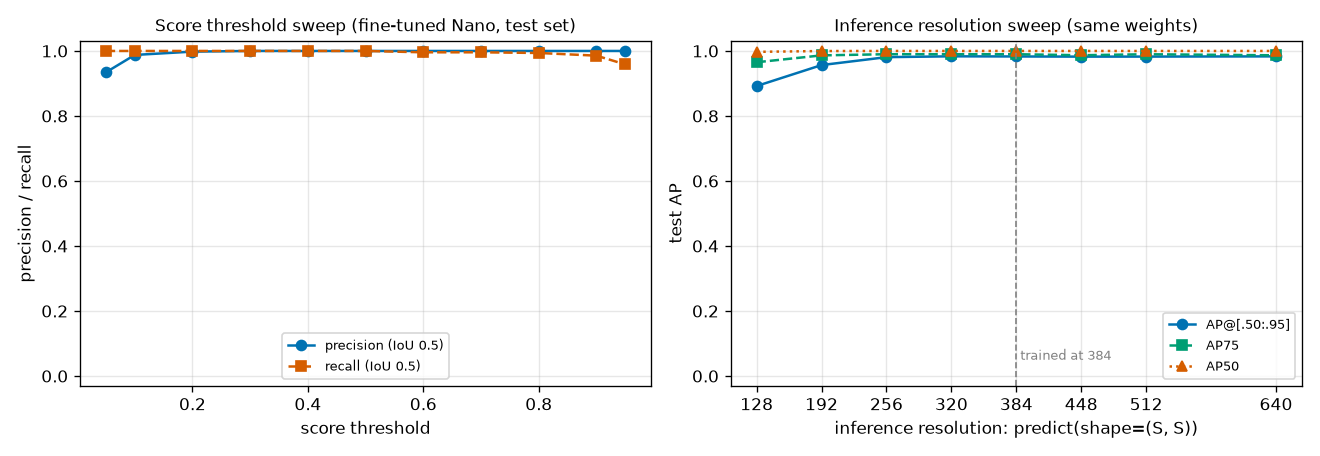
The left panel shows precision (blue solid line) and recall (orange dashed line) as the score threshold rises, at IoU 0.5. The right panel shows test AP, AP50, and AP75 when only the inference resolution is changed with predict(shape=(S, S)); the gray vertical line marks the training resolution of 384.
Score threshold
predict(threshold=…) keeps only predictions scoring above that value. Raising the threshold reduces wrong predictions (precision ↑) and increases missed objects (recall ↓). It is the same trade-off as in Chapter 3.
- From 0.3 to 0.5 it is perfect. Exactly 483 predictions remain, equal to the number of ground-truth objects, and precision and recall are both 1.0000 (at IoU 0.5). The default of 0.5 suits this data well.
- Lowering it mixes in false positives. At 0.05, the predictions grow to 517, 34 of which are wrong, so precision is \(483/517 = 0.934\). Recall is already 1, so there is nothing more to gain.
- Raising it causes misses. 476 at 0.9 (recall 0.986) and 463 at 0.95 (recall 0.959). This means there are 20 objects that the model found correctly but didn't score as high as 0.95.
- You can also see that the scores are split toward the two extremes. Of the tens of thousands of predictions from the 200 images, only 517 exceed 0.05, and between 0.2 and 0.8 the count barely changes (484 → 480). That is why the two lines in the left panel of Figure 14-6 stay at 1 over a wide range.
Real data won't produce such a wide, flat range. Build a table like this on the validation set and set the threshold depending on “whether false alarms or misses are worse”. The threshold does not affect AP (AP is computed by sweeping over all thresholds). According to the docstring, you can also pass ClassThresholds to threshold to use a different threshold per class (not tried).
Number of predictions kept: num_select
This is the number of (query, class) pairs that postprocessing keeps. It can be changed even after the model is created, with model.model.postprocess.num_select = K.
- Cutting it from 300 to 20 leaves AP unchanged (0.9830). Each image has at most 4 objects, and their predictions sit at the very top of the score ranking. Even cutting it to 5 gives 0.9819.
- Cutting it to 2 makes AP collapse (0.7116). Naturally so: in images with 3 – 4 objects, the model can give only two answers.
num_selectmust be comfortably larger than “the maximum number of objects that can appear in one image”. - Asking for 300 predictions but getting 250.7 on average is because our
detections_to_predictionfiltered out the predictions for the unused fourth slot. On average about 49 of the top 300 pairs were in that slot.
Reducing num_select doesn't reduce the network's computation (all 300 queries still pass through the decoder). Only the postprocessing and the size of the results shrink. Reducing the computation itself is the “number of queries” knob from Chapter 12, which changes the model architecture, so this chapter doesn't cover it.
Inference resolution
predict(shape=(H, W)) changes the input resolution for that call only. Neither the weights nor the model configuration change.
- AP is nearly the same from 256 to 640 (0.981 – 0.9835, within 0.003). The model was “trained at 384”, but through multi-scale training it actually saw many sizes from 224 to 544, and the positional embeddings are interpolated to fit the size. Even at 640, a size never seen in training, it scores 0.9833. Treating resolution as “a knob you can turn after training”, as in Chapter 12, holds up on the real model too.
- Going too low hurts. 0.957 at 192 and 0.892 at 128. Yet even at 128, AP50 is 0.997. The model doesn't miss objects; rather, the boxes become less precise (AP75 0.965). At 128 there are only \(8 \times 8 = 64\) patches, so compared with the 576 at 384, the grid along each side is three times coarser.
- Going higher doesn't help either. The original images are 192 pixels, so enlarging them beyond 384 adds no new information. Results would differ for large photos with many small objects.
- The times in the rightmost column include file reading and were measured while the GPU was shared, so they are for reference only (they fluctuate enough that 512 came out slower than 640). Still, the trend of increasing with resolution (11.5 ms at 128, 24.9 ms at 384, 42.3 ms at 640) is visible. A lower resolution is an option that is “a little less accurate and faster”.
- 400, which is not a multiple of 32, is rejected as seen earlier (the last line of the output).
- When the resolution can't be changed
- Inference-only snapshots created with
model.inference()and exported ONNX files have a fixed resolution. To use a different resolution, recreate or re-export them at that resolution.
Export and deployment
A trained model runs only inside PyTorch. In real services and on devices, models are often run without PyTorch, on a runtime tuned for the hardware. Converting a model into a file that another runtime can read is called export. ch14_export.py exports the fine-tuned Nano, runs it on another runtime, and measures its speed.
Exporting to ONNX
ONNX (Open Neural Network Exchange) is a file format that describes a neural network as “a graph of standard operations”. Once a model built in PyTorch is written to an ONNX file, any of the many runtimes that can read ONNX (ONNX Runtime, TensorRT, OpenVINO …) can run it. It is a kind of common language between different tools. The list of standard operations grows a little with each version, and that version number is called the opset (operator set version).
In the package this is one line, model.export(). The installed version's default arguments are format="onnx", opset_version=17, batch_size=1, and output_dir="output", and it returns the path of the exported file.
ch14_export.py · export
print(f"[2] ONNX 로 내보내기 → {EXPORT_DIR}/")
start = time.time()
onnx_path = model.export(output_dir=EXPORT_DIR, verbose=False)  # 기본값: format="onnx", opset_version=17, batch_size=1
print(f"  model.export() 가 돌려준 경로: {onnx_path}  ({time.time() - start:.1f}초,"
      f" {os.path.getsize(onnx_path) / 2**20:.1f} MB)")
graph = onnx.load(str(onnx_path))
print(f"  opset {graph.opset_import[0].version}, 노드 {len(graph.graph.node)}개")
options = ort.SessionOptions()
options.intra_op_num_threads = CPU_THREADS  # 연산 하나를 몇 개의 스레드로 나눠 계산할 것인가
session = ort.InferenceSession(str(onnx_path), options, providers=["CPUExecutionProvider"])
for tensor in session.get_inputs():
    print(f"  입력  {tensor.name!r}: 모양 {tensor.shape}, {tensor.type}")
for tensor in session.get_outputs():
    print(f"  출력  {tensor.name!r}: 모양 {tensor.shape}, {tensor.type}")
meta = json.loads({p.key: p.value for p in graph.metadata_props}["rfdetr_inference"])
shown = ("input_shape", "means", "stds", "channel_order", "resize_interpolation", "resize_antialias",
         "outputs", "box_format", "class_names", "num_select")
print("  파일에 함께 적힌 메타데이터(일부):", json.dumps({k: meta[k] for k in shown}, ensure_ascii=False))
[0] 환경: rfdetr 1.12.1, torch 2.15.0+cu132, onnx 1.23.2, onnxruntime 1.32.0 (실행 제공자 ['AzureExecutionProvider', 'CPUExecutionProvider'])
  GPU: NVIDIA RTX PRO 2000 Blackwell Generation Laptop GPU | CPU: Intel(R) Core(TM) Ultra 7 255H (코어 16개)
[1] 모델: fine-tuned Nano (Shape World, 3 classes), 입력 해상도 384×384
[2] ONNX 로 내보내기 → ch14_export/
  model.export() 가 돌려준 경로: ch14_export/rfdetr-nano.onnx  (8.6초, 102.7 MB)
  opset 17, 노드 1422개
  입력  'input': 모양 [1, 3, 384, 384], tensor(float)
  출력  'dets': 모양 [1, 300, 4], tensor(float)
  출력  'labels': 모양 [1, 300, 4], tensor(float)
  파일에 함께 적힌 메타데이터(일부): {"input_shape": [1, 3, 384, 384], "means": [0.485, 0.456, 0.406], "stds": [0.229, 0.224, 0.225], "channel_order": "RGB", "resize_interpolation": "bilinear", "resize_antialias": false, "outputs": {"pred_boxes": "dets", "pred_logits": "labels"}, "box_format": "cxcywh_normalized", "class_names": ["circle", "rectangle", "triangle"], "num_select": 300}
- The output. A single file,
rfdetr-nano.onnx(102.7 MB). The repository documentation (development version) mentions the nameinference_model.onnx, but 1.12.1 names the file after the model type. Don't guess the name in advance; use the path thatexport()returns. - The input is named
input, with shape[1, 3, 384, 384], float32. The batch size of 1 and the resolution of 384 are fixed in the graph. According to the docstring, for a different batch size you re-export withexport(batch_size=4)orexport(dynamic_batch=True), and for a different resolution withexport(shape=(H, W))(the same divisibility constraint applies). - There are two outputs,
dets(boxes,[1, 300, 4]) andlabels(class logits,[1, 300, 4]). They are exactly the raw outputspred_boxesandpred_logitsseen earlier, and neither preprocessing nor postprocessing is included in the graph. Resizing, normalization, and top-K selection are up to the caller. - Metadata. That's why the package writes the information needed for preprocessing and postprocessing (mean and standard deviation, channel order, interpolation method, output names, box format, class names,
num_select) into the ONNX file itself. Even if you are handed only the one file, you can tell how to use it.
- Tell the outputs apart by name, not by shape
- Our model's two outputs have exactly the same shape,
[1, 300, 4]: the boxes because they have 4 coordinates, and the logits because there are 3 classes + 1 slot. Code that picks an output by its shape, such as “the one whose last dimension is 4 is the boxes”, silently goes wrong precisely when there are 3 classes (the official documentation also warns about this trap). Fetch the outputs by name, as insession.run(["dets", "labels"], …).
Running with onnxruntime and comparing with PyTorch
ONNX Runtime (onnxruntime) is an engine that executes ONNX graphs. The hardware that does the computation is chosen via an “execution provider”. The base onnxruntime package installed by rfdetr[onnx] has no GPU provider (CUDA is absent from the provider list on the first line of the output above). Running on GPU requires onnxruntime-gpu separately. This chapter used only the CPU provider.
The first thing to check is that the exported model performs the same computation as the original. We feed the same input tensor to the PyTorch model and the ONNX model and compare the raw outputs numerically. Preprocessing is done directly with the preprocess function seen earlier.
ch14_export.py · parity
print("[3] onnxruntime 추론 vs PyTorch 순전파 (같은 입력 텐서)")
image = np.asarray(Image.open(test_paths[0]).convert("RGB"))  # (192, 192, 3) uint8
height, width = image.shape[:2]
reference = model.predict(test_paths[0], threshold=0.5)        # 비교 기준. (처음 부를 때 모델이 GPU 로 옮겨진다)
x = preprocess(image, size, model.means, model.stds)           # (1, 3, 384, 384)
dets, logits = session.run(["dets", "labels"], {"input": x})   # 이름으로 꺼낸다: 둘 다 (1, 300, 4) 일 수 있다!
net = model.model.model.eval()                                  # 실제 nn.Module. eval() 을 잊지 않는다
with torch.no_grad():
    out = net(torch.from_numpy(x).to(model.model.device))      # {"pred_boxes": (1, 300, 4), "pred_logits": (1, 300, C)}
torch_boxes = out["pred_boxes"].float().cpu().numpy()[0]        # (300, 4)
torch_logits = out["pred_logits"].float().cpu().numpy()[0]      # (300, C)
box_diff = np.abs(dets[0] - torch_boxes).max(axis=1)            # 질의마다의 박스 차이 (300,)
logit_diff = np.abs(logits[0] - torch_logits).max(axis=1)
best = (1.0 / (1.0 + np.exp(-logits[0]))).max(axis=1)           # 질의마다의 최고 점수 (300,)
confident = best > 0.05                                         # "쓸모 있는" 질의
differ = box_diff > 1e-3
r, g, b = (int(v) for v in image[0, 0])
print(f"  전처리 예: 왼쪽 위 픽셀 RGB ({r}, {g}, {b}) → 정규화 뒤 {[round(float(v), 4) for v in x[0, :, 0, 0]]}"
      f"  (R 채널 손계산: ({r}/255 − 0.485)/0.229 = {(r / 255 - 0.485) / 0.229:.4f})")
print(f"  입력 {x.shape} → dets {dets.shape}, labels {logits.shape}")
print(f"  check (점수 0.05 초과 질의 {int(confident.sum())}개): 박스 최대 차이 {box_diff[confident].max():.1e},"
      f" 로짓 최대 차이 {logit_diff[confident].max():.1e}  (PyTorch {device} vs onnxruntime CPU)")
print(f"  질의 300개 전체: 박스 최대 차이 {box_diff.max():.1e}, 로짓 최대 차이 {logit_diff.max():.1e}"
      f" | 박스 차이가 1e-3 을 넘는 질의 {int(differ.sum())}개, 그 질의들의 최고 점수 {best[differ].max() if differ.any() else 0.0:.3f}")
diff_boxes, diff_logits = float(box_diff[confident].max()), float(logit_diff[confident].max())
[3] onnxruntime 추론 vs PyTorch 순전파 (같은 입력 텐서)
  전처리 예: 왼쪽 위 픽셀 RGB (30, 17, 39) → 정규화 뒤 [-1.6042, -1.7381, -1.1247]  (R 채널 손계산: (30/255 − 0.485)/0.229 = -1.6042)
  입력 (1, 3, 384, 384) → dets (1, 300, 4), labels (1, 300, 4)
  check (점수 0.05 초과 질의 4개): 박스 최대 차이 7.8e-05, 로짓 최대 차이 1.3e-02  (PyTorch cuda vs onnxruntime CPU)
  질의 300개 전체: 박스 최대 차이 1.0e+00, 로짓 최대 차이 2.3e+00 | 박스 차이가 1e-3 을 넘는 질의 185개, 그 질의들의 최고 점수 0.013
Let's read the two check lines of the output in turn.
- They agree on the queries that caught objects. On the 4 queries scoring above 0.05 (the 4 objects in this image), the maximum box difference is \(7.8 \times 10^{-5}\) (normalized units; 0.015 pixels in a 192-pixel image) and the maximum logit difference is 0.013. It is normal for these not to be exactly 0. One side is PyTorch on the GPU and the other ONNX Runtime on the CPU, so the same formulas are computed in different orders by different libraries, and since float32 has only about 7 significant digits, the last digits drift slightly over dozens of layers. A logit difference of 0.013 amounts to a score difference of about 0.0003 near a score of 0.98.
- But comparing all 300 queries shows large differences. The maximum box difference is 1.0 and the maximum logit difference 2.3. As many as 185 queries differ by more than \(10^{-3}\). Did the export go wrong? No. Even the highest score among those 185 queries is just 0.013. They are all background queries that answered “there is nothing here”.
- Why only the background queries differ. Recalling the two-stage query selection of Chapter 10 suggests the reason. Among the proposals from the 576 positions (24 × 24) of the encoder output, the top 300 by score become the queries' reference boxes. In Shape World the background looks much the same everywhere, so the proposal scores of background positions are nearly equal, and a tiny change in the last digits caused by a different computation order is enough to swap their ranking. The same query index then receives a different proposal, and its output changes entirely. Proposals on objects have clearly higher scores, so their ranking doesn't change. (This explanation is an inference consistent with the observations; it was not verified by comparing the proposal rankings directly.)
- When validating an exported model
- Comparing the raw output tensors wholesale with
np.allclosecan flag a perfectly fine model as “different”. Compare only the useful predictions (those scoring above the threshold), or compare the detection results after postprocessing, as in the next section. The most reliable check is to re-measure AP on the whole validation set with the exported model. If even the useful predictions differ by something as large as 0.1, then the preprocessing differs (RGB order, normalization, interpolation method) oreval()was left out.
Postprocessing the raw outputs yourself
Now we feed the dets and labels from ONNX into the postprocess function built earlier to turn them into detection results, and compare them with the results of model.predict(). Since all three stages — preprocessing → ONNX forward pass → postprocessing — were done by our own code, a match here means the same results can be produced somewhere with neither PyTorch nor the rfdetr package (for example, on a server written in another language).
[4] 날출력을 직접 후처리 vs model.predict()
  로짓 (Q, C) = (300, 4) → 쌍 1200개 가운데 상위 300개 → 문턱값 0.5 를 넘는 것 4개
    질의   1 · 클래스 1 (rectangle): 점수 0.9796, xyxy [10.5, 44.1, 75.8, 81.1]
    질의   0 · 클래스 1 (rectangle): 점수 0.9768, xyxy [88.4, 45.3, 148.8, 123.6]
    질의   2 · 클래스 0 (circle): 점수 0.9751, xyxy [118.9, 16.7, 162.1, 58.0]
    질의   3 · 클래스 1 (rectangle): 점수 0.9624, xyxy [59.2, 103.9, 116.1, 139.1]
  check: predict() 와 개수 같음 True, 클래스 같음 True, 박스 최대 차이 9.0e-03 픽셀, 점수 최대 차이 3.7e-05
  질의마다 가장 높은 점수의 분포: 0.5 초과 4개, 0.05 이하 296개 (질의 300개 가운데)
- The hand-written postprocessing matches
predict(). 4 detections with the same classes, a maximum box difference of 0.009 pixels, and a maximum score difference of \(3.7 \times 10^{-5}\). This is the PyTorch (GPU) vs. ONNX Runtime (CPU) computation difference from the previous section, carried over as is. From the 1,200 (query, class) pairs, 300 were selected, and 4 of them exceeded the threshold of 0.5. - The scores are split toward the two extremes. Of the 300 queries, 4 have a top score above 0.5 and 296 have a top score of 0.05 or less, with none in between. This is why there are no duplicates even without NMS (Chapter 7), and why a threshold of 0.3 or 0.5 gave the same results. It is also no coincidence that the queries that caught the objects are numbered 0, 1, 2, and 3. Two-stage query selection takes the encoder proposals in descending order of score and assigns them to queries 0, 1, 2 … in turn (Chapter 10), so the proposals at object locations get the lowest indices.
- There is also an easier route. If you load the ONNX file with the package's predictor, as in
RFDETRInference("…/rfdetr-nano.onnx").predict(image), it handles preprocessing and postprocessing by itself using the metadata in the file and returnsDetections(confirmed in 1.12.1 to produce the same boxes). If you can install the rfdetr package in your environment, this route is the safer one.
Measuring latency
In Chapter 12, latency was one axis of the NAS. But unlike AP, latency is a number that can differ several-fold depending on how it is measured. That is why the RF-DETR paper (Section 4, Appendix K) takes care to describe its measurement method. The first thing to decide is what to measure.
- Forward pass only (model only): the time for one pass through the network, with the preprocessed tensor already on the GPU. The tables in the paper and the README report this value.
- End to end: from receiving an image through preprocessing → forward pass → postprocessing to returning the result. This is the time a user actually waits.
There are also some tricks to measuring. The measure function below embodies them.
ch14_export.py · timer
def measure(run, warmup: int, repeats: int, sync=None, sleep: float = 0.0) -> np.ndarray:
    """run() 을 warmup 번 헛돌린 뒤 repeats 번 재서, 한 번마다 걸린 시간(ms)의 배열을 돌려준다.

    sync:  GPU 는 명령을 "예약" 만 하고 바로 돌아오므로, 재기 전후에 torch.cuda.synchronize 로 끝나기를 기다려야 한다.
    sleep: 순전파 사이에 쉬는 시간(초). 논문은 GPU 가 전력 제한에 걸리지 않게 200 ms 를 쉬었다.
    """
    for _ in range(warmup):
        run()
    if sync:
        sync()
    times = np.zeros(repeats)
    for i in range(repeats):
        if sleep:
            time.sleep(sleep)
        start = time.perf_counter()
        run()
        if sync:
            sync()
        times[i] = (time.perf_counter() - start) * 1000.0
    return times

def summarize(times: np.ndarray) -> dict:
    return {"median": float(np.median(times)), "p10": float(np.percentile(times, 10)),
            "p90": float(np.percentile(times, 90)), "mean": float(times.mean()), "n": int(len(times))}
- Discard the warm-up runs. The first few runs are much slower because of preparation work such as memory allocation, choosing operator implementations, and filling caches. These values must not go into the average. This exercise runs a few throwaway passes every time it switches configurations, and only then measures.
- Wait for the GPU. PyTorch's GPU operations work by “handing off the work and returning immediately”. If you read the clock without waiting for the work to finish with
torch.cuda.synchronize(), you only measure the time it took to hand off the work, and get absurdly fast values. - Measure many times and look at the distribution. A single value is swayed by whatever other programs happened to be doing at that moment. Each configuration is measured 200 times (40 times for CPU configurations), the median is used as the representative value, and the 10% and 90% percentiles are reported alongside to show the spread (the mean gets dragged by occasional large spikes).
- Batch 1. The latency of real-time detection is the time from one image arriving until its result comes out, so it is measured with a batch size of 1.
- Interleave the configurations being compared. When the machine is shared with other jobs, the load changes from moment to moment. If you measure configuration A completely and then B, “whether the machine happened to be idle at the time” leaks into the results. This exercise treats measuring every configuration a little (20 times for GPU configurations, 4 times for CPU ones) as one round and runs 10 rounds. Changes in load then affect all configurations evenly. Of course, it is best to measure on a machine with nothing else running.
The paper points out three measurement pitfalls. They are also things to check every time you read someone else's latency numbers.
| Pitfall | What happens | The paper's remedy |
| Power throttling | Running forward passes without a break heats up the GPU, which then slows itself down, making the measurements fluctuate | Rest 200 ms between forward passes. Resting longer than 200 ms reportedly made no difference |
| Mixing precisions in reports | Accuracy is measured with an FP32 model and latency with an FP16 (half precision, 16-bit floating point) engine, and both go into one table. But switching to FP16 can change accuracy — the paper notes that converting D-FINE to FP16 as is made its AP collapse to 0.5 | Measure and report accuracy and latency with the same artifact (the same FP16 engine) |
| Measuring without NMS | The YOLO family requires NMS after the network, but its time is often left out of the measurement | For models that need NMS, include its time in the comparison. DETR-family models have no NMS |
Here, FP16 is floating point that stores each number in 16 bits (half precision). Compared with the usual FP32 (32 bits, about 7 significant digits), it has only 3 – 4 significant digits, but it uses half the memory and computes faster on GPUs. Converting weights and intermediate values to numbers with fewer bits like this, to make a model smaller and faster, is collectively called quantization (FP32 → FP16, or further to 8-bit integers, INT8). The “engine” in the table is one built by TensorRT (NVIDIA TensorRT). TensorRT is NVIDIA's inference optimization tool: it takes an ONNX graph, fuses operations for a specific GPU, chooses precisions, picks the fastest implementations, and compiles the result into an “engine” file. All latencies in the paper were measured with FP16 engines built with TensorRT 10.4 on a T4 GPU.
Results measured on this laptop
The fine-tuned Nano (384 × 384) was measured on this tutorial's laptop (NVIDIA RTX PRO 2000 Blackwell laptop GPU with 8 GB, Intel Core Ultra 7 255H with 16 cores). One thing must be stated up front: these measurements were taken while other training jobs were using the same GPU and CPU. These are poor conditions for measuring latency, but they make it possible to see in numbers “how much the measurements are swayed by conditions”.
ch14_export.py · latency
print("[5] 지연 시간 (배치 1, 그림 1장당 ms)")
rounds = 2 if args.quick else 10              # 구성들을 이 횟수만큼 번갈아 돌며 잰다
gpu_n, cpu_n = (5, 2) if args.quick else (20, 4)  # 한 라운드에서 구성 하나를 재는 횟수 (GPU, CPU)
x_cpu = torch.from_numpy(x)
default_threads = torch.get_num_threads()     # PyTorch 의 기본 스레드 수 (보통 코어 수)
configs = []                                  # 잴 구성의 목록: 이름 · 실행할 함수 · 한 라운드의 횟수 …

def add(label, key, run, n, device_kind="gpu", sleep=0.0, threads=None):
    configs.append({"label": label, "key": key, "run": run, "n": n, "device": device_kind, "sleep": sleep,
                    "threads": threads})

if device == "cuda":
    x_gpu = x_cpu.cuda()

    def forward_fp16():
        with torch.autocast("cuda", dtype=torch.float16):  # 자동 혼합 정밀도: 되는 연산은 FP16 으로
            return net(x_gpu)

    with torch.no_grad():
        out16 = forward_fp16()
    keep = torch.from_numpy(confident).to(x_gpu.device)  # 점수 0.05 초과 질의만 비교 (이유는 [3] 과 같다)
    print(f"  FP16 과 FP32 의 출력 차이 (점수 0.05 초과 질의):"
          f" 박스 최대 {float((out16['pred_boxes'].float() - out['pred_boxes'])[0][keep].abs().max()):.1e},"
          f" 로짓 최대 {float((out16['pred_logits'].float() - out['pred_logits'])[0][keep].abs().max()):.1e}")
    add("PyTorch GPU FP32, forward only", "torch_gpu_fp32", lambda: net(x_gpu), gpu_n)
    add("PyTorch GPU FP16 autocast, forward only", "torch_gpu_fp16", forward_fp16, gpu_n)
    add("PyTorch GPU FP32, forward only, 200 ms sleep between", "torch_gpu_fp32_sleep", lambda: net(x_gpu),
        max(2, gpu_n // 4), sleep=0.2)
    add("PyTorch GPU FP32, model.predict() end to end", "torch_gpu_predict",
        lambda: model.predict(image, threshold=0.5, include_source_image=False), gpu_n)
    # 패키지가 권하는 추론 전용 스냅숏: 고정 배치 · 고정 해상도로 추적(trace)해 CUDA 그래프로 재생한다.
    # 준비가 길어(분 단위) --quick 에서는 건너뛴다.
    for dtype, tag in (() if args.quick else (("float32", "FP32"), ("float16", "FP16"))):
        start = time.time()
        predictor = model.inference(dtype=dtype)  # RFDETRInference 를 돌려준다 (원래 model 은 그대로)
        print(f"  model.inference(dtype={dtype!r}) 준비 {time.time() - start:.1f}초")
        add(f"PyTorch GPU {tag}, model.inference() predictor end to end", f"torch_gpu_predictor_{tag.lower()}",
            lambda predictor=predictor: predictor.predict(image, threshold=0.5), gpu_n)
        if dtype == "float16":
            half = predictor.predict(image, threshold=0.5)
            print(f"  FP16 스냅숏의 예측: {len(half)}개, predict() 와 박스 최대 차이"
                  f" {float(np.abs(half.xyxy - reference.xyxy).max()) if len(half) == len(reference) else float('nan'):.2f} 픽셀")
net_cpu = net if device == "cpu" else copy.deepcopy(net).cpu()
add(f"onnxruntime CPU FP32 ({CPU_THREADS} threads), forward only", "ort_cpu_fp32",
    lambda: session.run(["dets", "labels"], {"input": x}), cpu_n, "cpu")
add(f"PyTorch CPU FP32 ({CPU_THREADS} threads), forward only", "torch_cpu_fp32", lambda: net_cpu(x_cpu), cpu_n, "cpu",
    threads=CPU_THREADS)
if default_threads != CPU_THREADS:
    add(f"PyTorch CPU FP32 ({default_threads} threads = default), forward only", "torch_cpu_fp32_default",
        lambda: net_cpu(x_cpu), 1, "cpu", threads=default_threads)

# 기계를 다른 작업과 나눠 쓰면 부하가 시시각각 변한다. 구성 A 를 다 재고 B 를 재면 "그때 기계가 한가했는가" 가
# 결과에 섞인다. 그래서 A, B, C … 를 조금씩 번갈아(라운드) 재서, 부하의 변화가 모든 구성에 고르게 묻게 한다.
print(f"  라운드 {rounds}번 · 구성 {len(configs)}개를 번갈아 잰다. 시작할 때: load average {os.getloadavg()[0]:.1f}"
      f" (CPU 코어 {os.cpu_count()}개), GPU 사용률 · 메모리 {gpu_utilization() or '-'}")
sync = torch.cuda.synchronize if device == "cuda" else None
collected = {c["key"]: [] for c in configs}
with torch.no_grad():
    for _ in range(rounds):
        for c in configs:
            if c["threads"]:
                torch.set_num_threads(c["threads"])
            is_gpu = c["device"] == "gpu"
            collected[c["key"]].append(measure(c["run"], 3 if is_gpu else 1, c["n"], sync if is_gpu else None, c["sleep"]))
torch.set_num_threads(default_threads)
print(f"  끝났을 때: load average {os.getloadavg()[0]:.1f}, GPU 사용률 · 메모리 {gpu_utilization() or '-'}")
# 라운드마다의 중앙값을 표로: 행 = 구성, 열 = 라운드. 어떤 라운드에서 모든 구성이 함께 느려졌다면 기계가 붐빈 것이다.
medians = np.array([[np.median(t) for t in collected[c["key"]]] for c in configs])  # (구성 수, 라운드 수)
relative = medians / np.median(medians, axis=1, keepdims=True)  # 구성마다 자기 중앙값으로 나눠 단위를 없앤다
quiet = int(relative.mean(axis=0).argmin())                     # 모든 구성이 전체적으로 가장 빨랐던 라운드
print("  라운드별 중앙값 (ms): " + " ".join(f"{'R' + str(r + 1):>8s}" for r in range(rounds)))
for c, row in zip(configs, medians):
    print(f"    {c['key']:22s}" + " ".join(f"{v:8.1f}" for v in row))
print(f"  가장 한가했던 라운드: R{quiet + 1}")
rows = []
print(f"  {'구성':58s} 전체 중앙값 |      10% |      90% | R{quiet + 1} 의 중앙값 | n")
for c, row in zip(configs, medians):
    times = np.concatenate(collected[c["key"]])
    stats = summarize(times)
    rows.append({"label": c["label"], "key": c["key"], "device": c["device"], "times": times.tolist(),
                 "round_medians": row.tolist(), "quiet": float(row[quiet]), **stats})
    print(f"  {c['label']:58s} {stats['median']:10.2f} | {stats['p10']:8.2f} | {stats['p90']:8.2f} |"
          f" {row[quiet]:12.2f} | {stats['n']}")
[5] 지연 시간 (배치 1, 그림 1장당 ms)
  FP16 과 FP32 의 출력 차이 (점수 0.05 초과 질의): 박스 최대 3.4e-05, 로짓 최대 4.7e-03
  model.inference(dtype='float32') 준비 85.6초
  model.inference(dtype='float16') 준비 88.7초
  FP16 스냅숏의 예측: 4개, predict() 와 박스 최대 차이 0.07 픽셀
  라운드 10번 · 구성 9개를 번갈아 잰다. 시작할 때: load average 4.8 (CPU 코어 16개), GPU 사용률 · 메모리 97 %, 3472 MiB
  끝났을 때: load average 13.7, GPU 사용률 · 메모리 70 %, 3474 MiB
  라운드별 중앙값 (ms):       R1       R2       R3       R4       R5       R6       R7       R8       R9      R10
    torch_gpu_fp32            15.2     16.9     17.5     16.9     16.7     16.9     16.7     16.9     17.2     17.3
    torch_gpu_fp16            14.1     12.0     14.0     11.3     15.5     14.8     14.1     12.6     15.9     11.7
    torch_gpu_fp32_sleep      18.1     18.6     20.8     19.7     20.4     19.4     19.5     20.9     21.2     18.1
    torch_gpu_predict         19.5     21.6     23.9     19.6     19.4     19.5     21.8     21.8     19.5     19.8
    torch_gpu_predictor_fp32    16.9     16.3     14.5     14.2     14.2     14.8     15.8     11.6     15.2     14.7
    torch_gpu_predictor_fp16    10.1     10.1      7.0     10.4     10.4      9.6     10.1     11.0     10.0     10.1
    ort_cpu_fp32             113.6    113.1    112.5    111.9    112.1    112.1    112.1    112.5    112.0    111.7
    torch_cpu_fp32           154.7    147.6    147.0    151.8    146.2    148.1    148.1    146.7    147.5    154.9
    torch_cpu_fp32_default  3428.0   3072.9   3082.1   2900.0   2939.1   3110.0   2940.0   3144.9   3007.1   3109.0
  가장 한가했던 라운드: R4
  구성                                                         전체 중앙값 |      10% |      90% | R4 의 중앙값 | n
  PyTorch GPU FP32, forward only                                  16.91 |    14.87 |    17.61 |        16.86 | 200
  PyTorch GPU FP16 autocast, forward only                         13.83 |    11.31 |    17.02 |        11.32 | 200
  PyTorch GPU FP32, forward only, 200 ms sleep between            19.67 |    17.09 |    21.94 |        19.71 | 50
  PyTorch GPU FP32, model.predict() end to end                    20.35 |    17.50 |    24.32 |        19.63 | 200
  PyTorch GPU FP32, model.inference() predictor end to end        14.61 |    12.28 |    17.77 |        14.24 | 200
  PyTorch GPU FP16, model.inference() predictor end to end        10.13 |     7.84 |    12.85 |        10.35 | 200
  onnxruntime CPU FP32 (8 threads), forward only                 112.29 |   111.67 |   115.56 |       111.95 | 40
  PyTorch CPU FP32 (8 threads), forward only                     147.96 |   146.46 |   160.51 |       151.78 | 40
  PyTorch CPU FP32 (16 threads = default), forward only         3077.49 |  2935.22 |  3173.22 |      2899.97 | 10
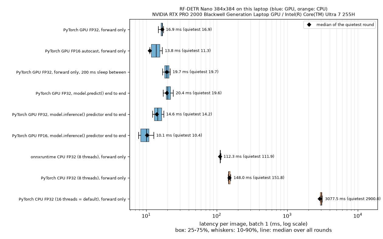
Box plots of the latency measured on the same model and the same single image, varying only the configuration (horizontal axis on a log scale). The boxes span 25 – 75%, the whiskers 10 – 90%, the line inside each box is the overall median, and the black diamond is the median of the round in which the machine was least busy. Blue marks GPU configurations and orange CPU configurations. The GPU configurations cluster between a few and a few tens of milliseconds, while the CPU configurations sit much further to the right, with widely spread boxes.
The upper table in the output gives the median for each round. If the values in each row (configuration) are even across the columns, the machine's conditions didn't change much during the measurement, and that was the case for this run. The lower table can be summarized as follows.
| Configuration | What was measured | Median (ms) | 10% – 90% |
| PyTorch GPU, FP32 | Forward pass only | 16.9 | 14.9 – 17.6 |
| PyTorch GPU, FP16 automatic mixed precision | Forward pass only | 13.8 | 11.3 – 17.0 |
| PyTorch GPU, FP32, 200 ms rest between runs | Forward pass only | 19.7 | 17.1 – 21.9 |
| | End to end | 20.4 | 17.5 – 24.3 |
| | End to end | 14.6 | 12.3 – 17.8 |
| | End to end | 10.1 | 7.8 – 12.9 |
| onnxruntime CPU, FP32, 8 threads | Forward pass only | 112.3 | 111.7 – 115.6 |
| PyTorch CPU, FP32, 8 threads | Forward pass only | 148.0 | 146.5 – 160.5 |
| PyTorch CPU, FP32, 16 threads (default) | Forward pass only | 3,077 | 2,935 – 3,173 |
- What you measure changes the result by 3.4 ms. For the same FP32 model, the forward pass alone takes 16.9 ms, while the whole of
predict()takes 20.4 ms. Preprocessing, postprocessing, and copying the results back to the CPU account for 17% of the total. Any claim of “N ms latency” should always come with “from where to where”. - FP16 is faster, and the output changes slightly. Just turning on automatic mixed precision cut the forward pass by 18%, from 16.9 to 13.8 ms. In exchange, the outputs change: on the queries that caught objects, by up to \(3.4 \times 10^{-5}\) for boxes and 0.0047 for logits. For this model that is negligible, but some models, like D-FINE in the paper, collapse in accuracy under FP16. This is why if you will run in FP16, you must re-measure AP in FP16.
- The inference-only snapshot is the fastest. The predictor created with
model.inference()takes 14.6 ms even with preprocessing and postprocessing included, faster than the forward pass alone of the general-purpose module (16.9 ms). The FP16 snapshot takes 10.1 ms, half ofpredict(). Its boxes differed from those ofpredict()by at most 0.07 pixels. The costs are the preparation time (85.6 and 88.7 seconds in this run; it took 12.7 seconds when the GPU was idle and up to 3 minutes when it was busy) and the fixed batch size and resolution. - Resting 200 ms actually made it slower (16.9 → 19.7 ms). On the paper's T4, running without a break triggered power throttling and made measurements fluctuate, hence the rest. On this laptop it was the opposite: during the rest, the GPU appears to drop into a power-saving state or other jobs grab the gap, so the next forward pass gets slower (the cause was not verified separately). Which value is “right” depends on the use case. For continuous input such as video, the former is closer to reality; for occasional single images, the latter is. That is why the measurement method must be reported along with the number.
- The CPU is an order of magnitude slower than the GPU, and the runtime matters. With the same 8 threads, onnxruntime takes 112 ms and PyTorch 148 ms, so onnxruntime is 1.3 times faster. That is 6.6 times the GPU forward pass (16.9 ms).
- The thread-count trap. By default, PyTorch uses as many threads as there are cores (16). Measured with that default, a single image took 3.1 seconds, 21 times as long as with 8 threads (148 ms). All ten rounds came in at 2.9 – 3.4 seconds. Other jobs were using some of the cores (load average 5 – 14), and this CPU mixes cores of different performance levels, so the 16 threads appear to spin idly waiting on one another. On a machine with nothing else running it may not get this bad (not verified), but “more threads means faster” cannot be relied on. If you deploy on a CPU, set
torch.set_num_threadsor onnxruntime'sintra_op_num_threadsyourself and measure. - When the machine is busy, everything fluctuates. In an earlier run of the same script while other jobs were in full swing (load average 25), the per-round median of the GPU FP32 forward pass ranged from 8.7 ms to 58.4 ms, and that of onnxruntime on CPU from 113 ms to 634 ms. The 8.7 ms of the fastest round then is probably close to the value with the GPU to yourself, whereas the 16.9 ms in the table above was measured with the GPU shared with other training. Compared with the paper's reported deviation of 0.1 ms on a dedicated T4, only about the first digit of the numbers in this table can be trusted.
- Don't compare these numbers with the 2.3 ms in the paper or README
- The “Nano 2.3 ms” in Table 2 of the paper and in the README is a value for NVIDIA T4 + TensorRT + FP16, forward pass only, batch 1. All of the following differ from the table above.
- Hardware: a T4 server GPU and a laptop GPU are different machines. Moreover, these measurements were taken while the GPU was shared with other training jobs.
- Runtime: a compiled TensorRT engine and a general-purpose PyTorch module (or ONNX Runtime on a CPU) run the same model at completely different speeds. This tutorial did not build a TensorRT engine.
- Precision: an FP16 engine vs. an FP32 forward pass.
- Scope: forward pass only vs. including preprocessing and postprocessing.
- Latency can be compared only between values measured on the same machine in the same way. The numbers your own service needs must be measured end to end on your hardware, with the runtime and precision you will actually use.
Other export formats
export(format=…) accepts many formats besides ONNX. The table below summarizes the installed version's export() docstring, the package's list of extras, and the official documentation. Only ONNX was actually run in this tutorial; the rest is based on the documentation.
| | Output | Extra install | Where it is used (per the documentation) |
| | | | Many runtimes, including ONNX Runtime. Verified directly |
| | | | Lowest latency on NVIDIA GPUs. Converted via ONNX; FP16 by default ( |
| | OpenVINO IR ( | | Intel CPUs, GPUs, and NPUs |
| | | | Mobile and edge. Converted ONNX → TensorFlow → TFLite |
| | | | The same file format as above, produced directly from PyTorch without ONNX or TensorFlow |
| | | | On-device PyTorch runtime. The target (xnnpack, coreml, qnn) must be set with |
| | | | Apple devices (Xcode) |
| | | | Apple Core AI (per the documentation: iOS, iPadOS, and macOS 27 or later) |
- The docstring warns that the TFLite, ExecuTorch, CoreML, and LiteRT exports are experimental and may change.
- INT8 quantization is done with
export(quantization="int8", calibration_data=…)(ONNX, OpenVINO, TensorRT). Converting to 8 bits requires knowing the range of the intermediate values, so calibration images similar to the images the model will actually see are essential. The documentation reports that ONNX INT8 lowered Nano's mAP by 2.65 on a subset of COCO (500 images) and advises “measuring on your own data before deployment”. - Whatever the format, the principle is the same as in this section: after exporting, always compare the outputs with the original model, and measure accuracy and latency together on the exported artifact itself.
Segmentation and keypoint models
RF-DETR-Seg, the model with the segmentation head built in Chapter 13, and a keypoint model (preview) that finds points such as human joints are also part of the same package. This section summarizes the official documentation and the installed version's source, and was not run directly.
| Detection | Instance segmentation | Keypoints (preview) | |
| Class | | | |
| Usage | The same: | ||
| What | | | |
| Dataset annotations | | | |
| Configuration (installed version) | Nano: 384 / patch 16 / 300 queries | SegNano: 312 / patch 12 / 1 window / 4 decoder layers / 100 queries | 576 / patch 12 / 4 decoder layers / 100 queries |
| Additional losses | – | Mask BCE and Dice losses ( | Keypoint loss |
| Criterion for choosing the best checkpoint | Box mAP | Mask mAP | Keypoint AP (OKS-based) |
In practice, using a segmentation model differs from detection in just two ways: the dataset annotations must include segmentation, and the results additionally contain detections.mask. Also keep in mind that, with a patch size of 12, the resolution must be a multiple of 24 (a multiple of 12 for SegNano). How the masks are produced (the dot product of query embeddings and pixel embeddings) and why they are computed at 1/4 of the resolution were built hands-on in Chapter 13.
Practical tips and common problems
This section collects only what was confirmed in this chapter's experiments and in the installed version's source and documentation.
- When memory runs out (CUDA out of memory)
-
- Reduce
batch_sizeand raisegrad_accum_stepsaccordingly to keep the effective batch size (4 × 4 → 2 × 8). This chapter's training withbatch_size=2used at most 1.61 GiB on Nano. - Use a smaller model (Nano) or a lower
resolution. The number of tokens is proportional to the square of the resolution (576 at 384, 1,024 at 512). - The documentation also lists
gradient_checkpointing=True(a setting passed when creating the model) as a way to reduce memory. It trades speed for memory, and was not tried in this chapter. - A large
num_workerscan exhaust main memory (RAM) rather than GPU memory.
- Reduce
- When small objects aren't detected
- Raising the resolution is the first remedy. At Nano's 384, one patch covers 16 × 16 pixels, so an object much smaller than that in the original image is only part of a single patch. Raise the resolution to a multiple of
patch_size × num_windows, as inmodel.train(resolution=512, …), or choose a size with a higher resolution from the start (Small 512, Medium 576, Large 704). As seen in Chapter 12, accuracy was more closely tied to “the number of patches per side” than to resolution or patch size on their own.
- Common stumbling blocks
-
- The resolution is rejected. If a side is not a multiple of
patch_size × num_windows(32 for Nano), you get aValueError. The same holds for training, inference, and export. - The class numbers seem shifted by one. A fine-tuned model's
class_idis not the JSONcategory_idbut a number reassigned from 0 in ID order. Only the COCO-pretrained model uses the 1 – 90 category IDs as is. - A warning that the number of classes doesn't match. “Checkpoint has 90 classes but model is configured for 3” is normal. Conversely, if you passed
num_classesto the model yourself, check that it matches the dataset. - Results with strange colors. numpy arrays must be in RGB order. If you read the image with OpenCV, flip BGR before passing it in.
- The validation folder name. It is
valid/, notval/, and the annotation file is_annotations.coco.json. - Calling train() again on the same model. According to the source, this does not continue training but starts over from the original pretrained weights, with a warning saying so. To continue, use
resume=. - Telling ONNX outputs apart by shape. With 3 classes, the boxes and the logits have the same shape. Fetch them by name (
dets,labels). - eval() when running the forward pass yourself. When you take out
model.model.model(the actualnn.Module) and use it directly, you have to call.eval()yourself.predict()does this for you. - Other people's latency tables. A latency figure that doesn't state the hardware, runtime, precision, and measurement scope cannot be used for comparison.
- The resolution is rejected. If a side is not a multiple of
- Where to start
-
- Run
predicton a few of your own images with the pretrained model (if that already works, you don't need training). - Put your data into COCO format, read the saved annotations back, and draw them on the images (as in Figure 14-3). If the annotations are wrong, everything after that is wasted effort.
- With the smallest model (Nano) and the default settings, run just a few epochs and see whether validation AP rises.
- Score on the test set and look at the predictions with your own eyes. Only if the results fall short, raise the resolution, the model size, or the number of epochs.
- Export, compare the outputs with the original model, and measure latency on the machine you will actually use.
- Run
Summary
- The
rfdetrpackage (version 1.12.1 in this chapter) is used through per-size classes (RFDETRNano…) and four methods:predict,train,evaluate, andexport. Training additionally requiresrfdetr[train], and ONNX requiresrfdetr[onnx]. Detection Nano – Large and the segmentation models are Apache 2.0; detection Atto, Femto, Pico, XLarge, and 2XLarge are PML 1.0 (rfdetr[plus]). -
predictresizes and normalizes the image to the model resolution and feeds it in, postprocesses the raw outputs in the order sigmoid → topnum_selectover all (query × class) pairs → threshold, and returns asupervision.Detections(xyxyin original pixels,confidence,class_id). There is no NMS. - Data is prepared in COCO format, with an
_annotations.coco.jsonin each of thetrain/ valid/ test/folders.bboxis pixel[x, y, w, h](relative to the top-left corner) and converts to and from normalized \((c_x, c_y, w, h)\) via \(x^{\text{px}} = (c_x - w/2)W\) and \(y^{\text{px}} = (c_y - h/2)H\). Class numbers are reassigned from 0 in category ID order. - Fine-tuning is the single line
model.train(dataset_dir=…), inside which the training loop from Chapter 11 runs. The effective batch size isbatch_size × grad_accum_steps, and the learning rate differs by component and layer, from 1e-4 for the head down to 3.2e-6 at the bottom of the backbone. In the logs,loss_ce,loss_bbox, andloss_giouare for the last decoder layer,_0marks the auxiliary losses, and_encthe losses on the encoder proposals. - In this tutorial's experiment, Nano started from the pretrained weights reached a validation AP of 0.95 after the first epoch and 0.984 after 5 epochs (test 0.983) on 1,000 Shape World images, while random initialization under the same conditions reached 0.77 after 3 epochs (test 0.772). The power of fine-tuning comes from pretraining.
- The package's
mAP_50_95has the same definition as Chapter 3's AP@[.50:.95]. Scoring the same predictions with ourevaluate_apagreed to within 0.002 (0.9828 vs. 0.9830, 0.7722 vs. 0.7738). - The exported ONNX model produces raw outputs (
dets,labels) without preprocessing or postprocessing. After exporting, compare its outputs numerically with the original model. Measure latency as the median of many runs, with warm-up and synchronization, and compare only on the same machine, runtime, precision, and scope.
Review questions
- 1. In an image 640 wide and 480 high, convert the normalized box \((c_x, c_y, w, h) = (0.25,\ 0.5,\ 0.5,\ 0.25)\) to a COCO
bbox. Then also write thatbboxin pixels in Chapter 2's corner format \((x_0, y_0, x_1, y_1)\). - \(x^{\text{px}} = (0.25 - 0.25) \times 640 = 0\), \(y^{\text{px}} = (0.5 - 0.125) \times 480 = 180\), \(w^{\text{px}} = 0.5 \times 640 = 320\), \(h^{\text{px}} = 0.25 \times 480 = 120\). So
bbox = [0, 180, 320, 120], and the corner format is \((0,\ 180,\ 0 + 320,\ 180 + 120) = (0, 180, 320, 300)\). The key points are that COCO's last two numbers are the width and height, not corner coordinates, and that horizontal values are multiplied by the width of 640 and vertical values by the height of 480.
- 2. You train on 2,400 training images with
batch_size=4,grad_accum_steps=4, andepochs=20. Find the effective batch size, the number of forward passes and weight updates per epoch, and the total number of updates. If GPU memory runs short and you have to reducebatch_sizeto 2, what do you change, and how, to keep the same effective batch size? - The effective batch size is \(4 \times 4 = 16\). Each epoch has \(2400/4 = 600\) forward passes and \(2400/16 = 150\) updates. The total is \(20 \times 150 = 3{,}000\) updates. If you reduce to
batch_size=2, raise it tograd_accum_steps=8to keep \(2 \times 8 = 16\). Forward passes per epoch rise to 1,200, but the number of updates stays at 150. Memory use goes down; time does not.
- 3. (a) From 400, 416, 500, and 640, choose the resolutions that can be used with RF-DETR Nano (
patch_size=16,num_windows=2). (b) Which of 384, 400, and 432 can be used with the segmentation model RFDETRSegSmall (patch_size=12,num_windows=2)? (c) How many patch tokens does Nano have at 640, and how many times as many as at 384? - (a) The resolution must be a multiple of \(16 \times 2 = 32\). \(416 = 32 \times 13\) and \(640 = 32 \times 20\) work; \(400/32 = 12.5\) and \(500/32 = 15.625\) don't. (b) Multiples of \(12 \times 2 = 24\): \(384 = 24 \times 16\) and \(432 = 24 \times 18\) work; \(400/24 = 16.67\) doesn't. (c) \(640/16 = 40\), so there are \(40 \times 40 = 1{,}600\) tokens. At 384 there are \(24 \times 24 = 576\), so it is \(1600/576 \approx 2.78\) times as many. The resolution grows by \(640/384 = 1.67\) times, but the number of tokens grows by its square.
- 4. The raw output
labelsof a Nano fine-tuned on 3 classes has shape(300, 4). (a) How many (query, class) pairs does postprocessing rank in total? (b) Which query and which class does the flattened index \(i = 1001\) correspond to? (c) If query 7's logits are \((3.0,\ 0.2,\ -4.0,\ -6.0)\) and the scores of all other queries are below 0.1, how many detections come from query 7 atthreshold=0.5, and what are they? - (a) \(300 \times 4 = 1{,}200\) pairs, of which the top 300 are selected. (b) \(q = \lfloor 1001/4 \rfloor = 250\) and \(c = 1001 \bmod 4 = 1\): class 1 (rectangle) of query 250. (c) The scores are \(\sigma(3.0) = 0.953\), \(\sigma(0.2) = 0.550\), \(\sigma(-4.0) = 0.018\), and \(\sigma(-6.0) = 0.002\). Two exceed 0.5, so the same box comes out twice: class 0 (circle) with a score of 0.953 and class 1 (rectangle) with a score of 0.550. Unlike the softmax approach, which picks only one class per query, sigmoid scores are independent for each slot, so this can happen. Raising the threshold to 0.6 leaves only one.
- 5. For Nano with the default settings (
lr_encoder=1.5e-4,lr_vit_layer_decay=0.8,lr_component_decay=0.7), compute the learning rate of backbone block 6. Then compute the EMA's effective decay rate \(d_t = 0.993\,(1 - e^{-t/100})\) at \(t = 50\) and \(t = 500\), and explain how the EMA behaves differently early and late in training. - Learning rate: \(1.5 \times 10^{-4} \times 0.7^2 \times 0.8^{13 - 6} = 7.35 \times 10^{-5} \times 0.8^7 = 7.35 \times 10^{-5} \times 0.2097 = 1.54 \times 10^{-5}\). EMA: at \(t = 50\), \(1 - e^{-0.5} = 0.3935\), so \(d = 0.993 \times 0.3935 = 0.391\). At \(t = 500\), \(1 - e^{-5} = 0.9933\), so \(d = 0.986\). Early on (\(d \approx 0.39\)), the EMA takes in as much as 61% of the new weights and follows them quickly; later (\(d \approx 0.99\)), it takes in only a little over 1% and moves slowly and smoothly. If \(d\) were 0.993 from the start, the EMA would stay stuck on the useless initial weights for a long time;
ema_tauprevents that.
- 6. A colleague says, “The README says Nano takes 2.3 ms, but when I measured
model.predict()on my laptop I got tens of milliseconds. I must have installed something wrong.” Give at least four reasons why the installation may not be at fault, and list what to check in the colleague's measurement. - The two numbers are measured under different conditions. ① Hardware: the README uses an NVIDIA T4, the colleague a laptop GPU (or a CPU). ② Runtime: the README uses an engine compiled with TensorRT, the colleague a general-purpose PyTorch module (without even using
model.inference()). ③ Precision: the README uses FP16, whilepredict()runs in FP32. ④ Scope: the README measures the forward pass only, whilepredict()includes image reading, preprocessing, postprocessing, and copying the results. Things to check: whether the warm-up runs were discarded; on a GPU, whether they waited for completion withtorch.cuda.synchronize(); whether they measured many times and looked at the median rather than measuring once; whether it is really running on the GPU (model.model.device); whether another program is using the GPU; and whether file-reading time is mixed in.
That concludes the main part of the tutorial. Starting from the coordinates of a single box, we assembled RF-DETR from parts we built ourselves, and finally fitted the real RF-DETR to our own data and exported it. The last chapter, Chapter 15 (Appendix), collects a checklist for when training isn't going well, a glossary of the terms and symbols used in this tutorial, and further reading for those who want to go beyond it.
See also
- RF-DETR:Tutorial
- RF-DETR
- RF-DETR:Review
- RF-DETR:Troubleshooting:SlowTraining
- DINOv2
- COCO
- PyTorch
- Object detection
Favorite site
- 14. Practice: the rfdetr package
- roboflow/rf-detr - Official repository (README, LICENSE, CHANGELOG)
- roboflow/supervision - The library that defines
Detections - ONNX Runtime
- RF-DETR: Neural Architecture Search for Real-Time Detection Transformers (arXiv:2511.09554)