RF-DETR:Tutorial:13-Segmentation
lastmod 2026-11-18created 2026-11-184 edits
RF-DETR-Seg: Instance Segmentation is chapter 13 of the RF-DETR tutorial. The detector built so far outputs one box per object. But half of a box that fits a triangle exactly, and a little over a fifth of a box around a circle, is background, and a box cannot tell where the boundary between overlapping objects lies. RF-DETR-Seg leaves the detector almost untouched and adds a single lightweight segmentation head so that it also outputs, for each object, the pixels that object occupies. The principle fits in one line: taking the dot product of an object query's embedding with a per-pixel embedding gives that object's mask. This chapter unpacks that line with equations and hand calculations, reads the segmentation head of the official implementation one layer at a time, and attaches the same head to the mini RF-DETR trained in chapter 11 to train it on the shapes world. It also uses the structure of the segmentation head to explain why the weight-sharing NAS of chapter 12 finds different configurations for segmentation models than for detection models.
- Original: 13. RF-DETR-Seg: Instance Segmentation (about 100 minutes to read, difficulty ★★★★☆)
- Practice code:
code/ch13_seg.py.python ch13_seg.pyattaches a segmentation head to the chapter 11 mini RF-DETR checkpoint (ch11_rfdetr.pt), trains it for 30 epochs, and runs the analysis (about 10 minutes on a laptop GPU).--analyzeregenerates only the tables and figures without training (about 35 seconds), and--ablationsruns the ablation experiments (about 8 minutes per seed). - Previous: 12. Weight-Sharing NAS / Next: 14. In Practice: the rfdetr Package
Notation in this chapter
- \(H, W\): height and width of the input image (pixels). \(h, w\): height and width of the feature map produced by the projector (cells). \(r\): the factor by which the mask resolution is reduced relative to the image (official setting name
mask_downsample_ratio, default 4). The mask logit grid is \(H/r \times W/r\). - \((x, y)\): one cell on the grid (column, row). In chapter 4 \(y\) was the ground-truth label, but in this chapter it is used only for vertical position, so the ground truth is written \(t\) (target).
- \(z\): logit, \(p = \sigma(z)\): probability, \(t \in \{0, 1\}\): ground truth. The subscript \(i\) indexes pixels (or sampled points), and \(P\) is their count.
- \(D\): hidden dimension (128 for the mini model, 256 for RF-DETR). \(N\): number of queries, \(n\): query index. \(L\): number of decoder layers, \(l\): layer index (starting from 1).
- \(B\): inside a tensor shape \((B, N, \dots)\), the batch size. Only in the IoU and Dice coefficient formulas does it denote the set \(B\) defined below.
- \(q_n\): the embedding of query \(n\) output by the decoder (a vector of length \(D\)). \(f(q_n)\): that vector after passing through the segmentation head's FFN. \(e(x, y)\): the pixel embedding of cell \((x, y)\) (length \(D\)). \(E\): the whole pixel embedding map, of shape \((D, H/r, W/r)\).
- \(\beta\): the bias added to the mask logits (a single scalar). The letter \(b\) was avoided because it is used for boxes.
- \(A\): the set of pixels where the predicted mask is 1, \(B\): the set of pixels where the ground-truth mask is 1. \(|A|\) is the number of pixels (in chapter 2 it was area).
- \(C\): the cost matrix for matching (chapter 7). The number of channels of a convolution is written \(D\) instead of \(C\).
From boxes to masks
When a box is not enough
Chapter 1 laid out three problems side by side. Image classification outputs one label for the whole image, object detection outputs a box per object, and instance segmentation outputs, per object, the pixels that object occupies. Chapters 2 through 12 solved only the middle problem. When is a box not enough?
Original figure 13-1 is a diagram with three panels showing a square, a circle, and a triangle, each enclosed in a dashed box. Below each panel is the ratio of shape area to box area: 1.00 for the square, \(\pi/4 \approx 0.785\) for the circle, and 0.50 for the triangle. Even a perfect box does not mean every pixel inside it belongs to the object.
The numbers in figure 13-1 can be worked out by hand. If the box has width \(w_b\) and height \(h_b\), its area is \(w_b h_b\).
- The triangle in the shapes world is an isosceles triangle with base \(w_b\) and height \(h_b\), so its area is \(\tfrac{1}{2} w_b h_b\), exactly half the box.
- The circle has diameter \(w_b = h_b\), so its area is \(\pi (w_b/2)^2 = \tfrac{\pi}{4} w_b^2\), which is \(\pi/4 \approx 0.785\) times the box.
- Only the square fills its box completely.
Because each shape lies entirely inside its box, the IoU of "answering with the box itself as the object's region" is intersection (shape) ÷ union (box), which equals the ratios above. Even if the triangle is found with a perfect box, using that box as the region gives an IoU of only 0.5. The cases where a box falls short come down to three.
- When the shape is not rectangular. When measuring area (the size of a defect, the leaf area of a crop), removing the background, or choosing where a robot should grasp, the background inside the box becomes error.
- When objects overlap. A box does not say which object the pixels in the overlap of two boxes belong to.
- Thin, tilted objects. For a rod lying diagonally, most of the box is background (absent from the shapes world but common in reality).
The mask as an output
The output of instance segmentation is three things per object: (class, box, mask). The class and box are the same as in detection; the mask is new. A mask is a grid the same size as the image with 0 or 1 written in each cell. 1 means "this pixel belongs to this object" and 0 means "it does not." If an \(H \times W\) image contains \(T\) objects, the ground-truth mask has shape \((T, H, W)\), one grid per object.
Ground-truth masks in the shapes world come from ShapesDataset(…, with_masks=True). The shape is (number of objects, 96, 96) and the dtype is bool. There is one convention: when a shape drawn later covers a shape drawn earlier, the covered pixels are removed from the mask of the underlying (earlier) shape. A mask is 1 only on the "actually visible part." So each pixel belongs to at most one object, and the mask of an occluded object is smaller than the original shape. The box stays the same (the box of the original shape, including the hidden part).
The model does not output 0/1 directly. Just like the binary classification of chapter 4, it outputs a logit \(z\) for each cell, turns it into a probability \(p = \sigma(z)\) with a sigmoid, and treats it as 1 if it exceeds 0.5. Since \(\sigma(0) = 0.5\) and the sigmoid is monotonically increasing, \(p \gt 0.5\) is the same as \(z \gt 0\). So at inference time there is no need to compute the sigmoid; only the sign of the logit matters.
| Stage | Value | Shape (\(N\) queries) |
| Mask logit | Real number. Larger means more "object" | \((N, H/r, W/r)\) |
| Probability | \(\sigma(z)\), between 0 and 1 | Same |
| Binary mask | 1 if \(z \gt 0\) | \((N, H, W)\) — upsampled to image size, then thresholded |
The \(r\) in the table stands out. RF-DETR-Seg computes masks not at image size but at a quarter of the resolution, and upsamples to image size only at the very end. The reason is covered when we look at the structure of the segmentation head.
IoU between masks
How well a predicted mask matches the ground truth is measured with the IoU of chapter 2. The definition is unchanged; the only difference is that area is counted in pixels. Let \(A\) be the set of pixels where the predicted mask is 1 and \(B\) the set where the ground-truth mask is 1. Then
\(\operatorname{IoU}(A, B) = \frac{|A \cap B|}{|A \cup B|} = \frac{\text{pixels where both are 1}}{\text{pixels where either is 1}}\)
This is called mask IoU. Box IoU was computed from four corner coordinates, while mask IoU is counted by comparing the two grids cell by cell. In code, it is the ratio of the sums of & and | of two boolean arrays.
The idea: dot products between queries and pixels
What happens if each pixel is predicted separately
The detector already has one object query per object (chapter 7). The query embedding \(q_n\) coming out of the decoder is a vector of length \(D\); a Linear layer on top of it gave the class, and an MLP gave the box. Can the mask be produced the same way? Consider attaching a Linear layer to the query embedding that outputs every cell of the mask at once.
The mask grid of RF-DETR-Seg Nano is 78×78 = 6,084 cells, and \(D = 256\). A single Linear layer has \(256 \times 6{,}084 = 1{,}557{,}504\) weights plus 6,084 biases, 1,563,588 parameters in total. The count is not the only problem.
- The number of output cells is baked into the shape of the weights, so it cannot be used if the resolution changes. The NAS of chapter 12 treats resolution as a knob.
- The boundary across 6,084 cells must be drawn from only the 256 numbers of the query embedding. Where an object's edges are is in the image's feature map, but that cannot be used directly.
- How to predict cell \((3, 5)\) and how to predict cell \((4, 5)\) are learned separately. The fact that neighboring cells are similar goes unused.
Queries ask, pixels answer
Change the idea. Instead of the query drawing every cell of the mask by itself, have the pixel side produce a vector for each cell as well.
- From the image's feature map, build a vector \(e(x, y)\) of length \(D\) for each cell of the mask grid. This is the pixel embedding, and the \((D, H/r, W/r)\) tensor collecting all cells is the pixel embedding map \(E\). It is built only once per image.
- Pass the query embedding \(q_n\) through a small FFN to get a vector \(f(q_n)\) of the same length, one per query.
- Whether cell \((x, y)\) belongs to query \(n\)'s object is decided by the dot product of the two vectors.
An analogy. Each pixel wears a name tag saying "I am part of something like this," and the query asks, "Pixels wearing a tag like this, raise your hand." Pixels whose tags match the question well (large dot product) raise their hands, and the set of raised hands is the mask. With 12 queries there are 12 questions, but only one set of name tags is needed.
- A mask built from dot products
- \(z_n(x, y) = \big\langle f(q_n),\ e(x, y) \big\rangle + \beta\)
- The logit that query \(n\) gives to cell \((x, y)\). \(\langle \cdot, \cdot \rangle\) is the dot product, and \(\beta\) is a single bias shared by all queries and all cells (a learned scalar, initialized to 0).
- The dot product written out: multiply the components of the two vectors position by position and sum. \(f(q_n)_c\) is the \(c\)-th component of the vector \(f(q_n)\), and \(e_c(x, y)\) is the \(c\)-th component of the pixel embedding. This is the same computation as the attention score in chapter 5, which was the dot product of a query and a key.
- Applying a sigmoid turns it into "the probability that this cell belongs to query \(n\)'s object." Unlike attention, this is a sigmoid rather than a softmax, because it is a separate yes/no decision for each cell and each query. So one cell can end up in the masks of two queries at once.
The formula can also be read another way. Asking whether \(z_n(x, y) \gt 0\) amounts to feeding the vector \(e(x, y)\) into a linear classifier with weights \(f(q_n)\) and bias \(\beta\) (a single neuron from chapter 4). An ordinary classifier's weights are fixed after training, but here the weights are created anew for every query and every image. In effect, the decoder writes "a classifier that picks out this object" on the spot.
Computing all queries and all cells at once is a single tensor operation. Including the batch, the shapes are as follows.
\(\underbrace{Z_{b,n,y,x}}_{(B,\, N,\, H/r,\, W/r)} \;=\; \sum_{c=1}^{D}\ \underbrace{E_{b,c,y,x}}_{(B,\, D,\, H/r,\, W/r)}\ \underbrace{F_{b,n,c}}_{(B,\, N,\, D)} \;+\; \beta\)
\(F\) stacks \(f(q_n)\) in query order, and the subscript \(b\) is the index of the image within the batch. In code it is one line: torch.einsum("bchw,bnc->bnhw", E, F) + bias. The letters in einsum name the axes, and the c axis, present on both inputs but absent from the result, is multiplied and summed over. That is exactly the \(\sum_c\) in the formula above. Counting what grows: whether there are 100 or 300 queries, there is one pixel embedding map, and whether the grid is 78×78 or 192×192, the shape of the weights stays the same. All three problems from the previous section are solved.
Computing a 2×2 grid by hand
Work through the smallest example: a 2×2 mask grid, 2-dimensional embeddings (\(D = 2\)), 2 queries, and \(\beta = 0\).
Original figure 13-2 is a diagram showing how one set of pixel embeddings and two query vectors produce two masks.
- Left: pixel embeddings \(e(x, y)\) on a 2×2 grid, a vector of length 2 in each cell. Top row \((2, 0)\), \((1, 1)\); bottom row \((0, 2)\), \((-1, -1)\).
- Middle: the query vectors and dot products.
- Right, first grid: query 1, \(f(q_1) = (2, -1)\). The logits in the cells are 4, 1 on the top row and −2, −1 on the bottom row.
- Right, second grid: query 2, \(f(q_2) = (-1, 1.5)\). The logits are −2, 0.5 on the top row and 3, −0.5 on the bottom row.
The number in each cell is the logit, and cells greater than 0 (shaded) form that query's mask. The top-right cell is in both masks.
- The four cells for query 1
- \(z_1(\text{top left}) = 2 \times 2 + (-1) \times 0 = 4\)
- The dot product of \(f(q_1) = (2, -1)\) and \(e = (2, 0)\): first components multiplied, second components multiplied, then summed.
- The dot product with \(e = (1, 1)\).
- The two bottom cells have negative logits, because their embeddings point away from \(f(q_1)\).
- Cells with probability above 0.5, that is, cells with positive logits, are 1. Query 1's mask is the top row.
Query 2 uses the same pixel embeddings. Computing with \(f(q_2) = (-1, 1.5)\) gives logits \(-2,\ 0.5,\ 3,\ -0.5\), and the mask is the top-right and bottom-left cells. The top-right cell is positive for both queries. Since each query decides independently, nothing prevents this kind of overlap; training merely pushes away from it. The code prints the same computation.
[손계산 1] 내적으로 만드는 마스크: 2×2 픽셀, 임베딩 2차원, 질의 2개
  질의 1 f(q) = [2.0, -1.0]: 로짓 [[4.0, 1.0], [-2.0, -1.0]] → 확률 [[0.982, 0.731], [0.119, 0.269]] → 마스크 [[1, 1], [0, 0]]
  질의 2 f(q) = [-1.0, 1.5]: 로짓 [[-2.0, 0.5], [3.0, -0.5]] → 확률 [[0.119, 0.622], [0.953, 0.378]] → 마스크 [[0, 1], [1, 0]]
Pixel embeddings are prototypes
Read the dot product again from the channel side. Taking only the \(c\)-th channel of the pixel embedding map \(E\) gives a single image \(E_c\) of size \((H/r, W/r)\). The whole logit map for query \(n\) is then
\(Z_n \;=\; \sum_{c=1}^{D} f(q_n)_c \; E_c \;+\; \beta\)
that is, a weighted sum of \(D\) images \(E_1, \dots, E_D\) with coefficients \(f(q_n)_c\). The images are shared by all objects; only the coefficients differ per object. Such shared base images are called prototypes. In the 2×2 example above there were two prototypes: the first channel \(\begin{pmatrix} 2 & 1 \\ 0 & -1 \end{pmatrix}\) and the second channel \(\begin{pmatrix} 0 & 1 \\ 2 & -1 \end{pmatrix}\), and query 1's logits were "twice the first minus the second." A negative coefficient means a prototype can also be subtracted.
The name comes from YOLACT (Bolya et al., 2019). YOLACT builds \(k\) prototype masks \(P\) (shape \(h \times w \times k\)) for the whole image, predicts \(k\) mask coefficients for each detected object, and combines the two with one matrix multiplication and a sigmoid. Equation (1) of the paper is \(M = \sigma(P C^{\top})\), where \(C\) is the \(n \times k\) matrix stacking the coefficients of \(n\) objects. It has the same form as the formula in this chapter. The YOLACT paper reports that performance does not drop even with only \(k = 32\) prototypes. The RF-DETR paper states in a single sentence that the pixel embeddings of its segmentation head "can be interpreted as segmentation prototypes (Bolya et al., 2019)." The experiments in this chapter will plot the channels of the pixel embeddings directly.
Similarities and differences with YOLACT
- Similarity: mask = (a map built once per image) × (a vector per object), fed into a sigmoid.
- Source of the coefficients: in YOLACT a convolutional head attached to each anchor outputs the coefficients (used only for objects kept after NMS), while RF-DETR-Seg builds them from the query embeddings output by the decoder. There is no NMS.
- Number of maps: YOLACT's \(k\) is a few dozen, while RF-DETR-Seg uses \(D = 256\), the same as the hidden dimension.
- YOLACT crops the combined mask with the predicted box. The official RF-DETR post-processing has no such step (confirmed from the source later).
Where it resembles MaskDINO, and where it differs
The RF-DETR paper states that its segmentation head was inspired by MaskDINO (Li et al., 2023). MaskDINO is the DETR-family detector DINO with a mask branch added, and it produces masks with equation (1) of its paper.
\(m = q_c \otimes \mathcal{M}\big(\mathcal{T}(C_b) + \mathcal{F}(C_e)\big)\)
\(q_c\) is the decoder's content query embedding and \(\otimes\) is the dot product. The term in parentheses is the pixel embedding map, built by adding a 1/4-resolution backbone feature map \(C_b\) to an upsampled version of the 1/8-resolution feature map \(C_e\) from the Transformer encoder (\(\mathcal{T}\) is a convolution that matches the channel count, \(\mathcal{F}\) is interpolation that upsamples \(C_e\) by 2×, and \(\mathcal{M}\) is the segmentation head). The skeleton, "dot product of query embeddings and a pixel embedding map," is the same as RF-DETR-Seg.
The difference is what goes into the pixel embedding map. In the words of the RF-DETR paper, "unlike MaskDINO, we do not feed multi-scale backbone features into the segmentation head, to reduce latency." The only input to RF-DETR-Seg is a single projector output: the very low-resolution map that the decoder's deformable cross-attention reads, upsampled with bilinear interpolation. Not bringing in fine high-resolution features separately may cost some boundary precision, but the computation of extracting and merging high-resolution maps from the backbone disappears entirely. In table 3 of the paper, MaskDINO (R50) reaches 46.3 COCO mask AP at 242 ms (measured with PyTorch), and RF-DETR-Seg (medium) reaches 45.3 at 5.9 ms (T4, TensorRT FP16).
The segmentation head of RF-DETR-Seg
Now turn the idea into actual layers. Everything about the structure in this section was read from rfdetr/models/heads/segmentation.py (class SegmentationHead) and models/lwdetr.py in the official repository. The paper describes the segmentation head in only one paragraph and figure 2, so the code is the reference for the layer composition.
Overall flow and tensor shapes
The segmentation head takes only two things from the detector: a single projector output, and the query embeddings from each decoder layer. The backbone, projector, decoder, classification head, and box head are identical, line for line, to chapter 10.
Original figure 13-3 is a diagram of the computation flow of the official SegmentationHead. The top row is the pixel side (once per image) and the bottom row is the query side.
- Pixel side: projector output \((B, D, h, w)\) → bilinear interpolation \((B, D, H/4, W/4)\) → depthwise convolution block 1 → block 2 → … → block \(L\). There is a separate block per layer, stacked in sequence. Applying a 1×1 convolution to the output of block \(l\) gives the pixel embedding map \(E_l\).
- Query side: queries from decoder layer \(l\) \((B, N, D)\) → MLP block → Linear.
- The dot product of the two plus the bias \(\beta\) is mask logit \(l\), with shape \((B, N, H/4, W/4)\).
- The 1×1 convolution, MLP block, Linear, and bias \(\beta\) are shared by all layers.
In other words, the query embeddings of the \(l\)-th decoder layer are dotted with the pixel embedding map \(E_l\), which has passed through \(l\) blocks.
Read figure 13-3 top to bottom, left to right.
- Upsample the projector output \((B, D, h, w)\) to \((B, D, H/4, W/4)\) with bilinear interpolation.
- Pass through the depthwise convolution blocks in sequence. There are as many blocks as decoder layers, and the output of block \(l\) is the input of block \(l + 1\).
- Applying one more 1×1 convolution to the output of block \(l\) gives the pixel embedding map \(E_l\) for layer \(l\).
- Pass the query embeddings from decoder layer \(l\) through the MLP block and Linear to get \(f(q)\).
- Take the dot product of \(E_l\) and \(f(q)\) and add the bias \(\beta\) to obtain the mask logits for layer \(l\), \((B, N, H/4, W/4)\).
Follow the shapes with RF-DETR-Seg Nano. These values were measured by hooking into the model from the installed rfdetr package (no trained weights were loaded; shapes and parameter counts do not depend on the weights).
[RF-DETR-Seg Nano 모양 추적] 설정: resolution 312, patch_size 12, num_windows 1, dec_layers 4, num_queries 100, hidden_dim 256, mask_downsample_ratio 4 (학습된 가중치는 싣지 않았다)
  그림                                               (1, 3, 312, 312)
  프로젝터 출력                                          (1, 256, 26, 26)
  쌍선형 보간 뒤 = 블록 1 의 입력                             (1, 256, 78, 78)
  블록 1 … 4 의 출력 (각각)                               (1, 256, 78, 78)
  1×1 합성곱 → 픽셀 임베딩 맵 (추론 때 1번 계산)                  (1, 256, 78, 78)
  질의 임베딩 → MLPBlock → Linear                       (1, 100, 256)
  pred_masks (마스크 로짓)                              (1, 100, 78, 78)
  pred_logits / pred_boxes                         ((1, 100, 91), (1, 100, 4))
  추론 모드의 보조 출력 키: ['pred_boxes', 'pred_logits'] × 3 (마스크는 마지막 층만 계산)
  매개변수: 전체 33,577,475개, 그 가운데 분할 머리 933,121개 (2.8%)
Dividing the resolution 312 by the patch size 12 gives a \(312 / 12 = 26\)-cell grid, and the mask grid is \(312 / 4 = 78\) cells. The projector output is upsampled 3× per side (9× in cell count). With 100 queries, the mask logits amount to \(100 \times 78 \times 78 = 608{,}400\) numbers per image. The segmentation head has 933,121 parameters, 2.8% of the model's 33,577,475. The total of 33.6M matches the parameter count for RF-DETR-Seg (nano) in table 3 of the paper. That is the actual size behind the phrase "lightweight segmentation head."
Upsampling with bilinear interpolation
Increasing the number of cells in a feature map is called upsampling. The values of the new cells have to be made from the values of the original cells, and the segmentation head uses the bilinear interpolation derived in chapter 8. For each cell center in the new grid, it takes a distance-weighted average of the four surrounding cells in the original grid. The official code is one line.
rfdetr/models/heads/segmentation.py (excerpt from the official implementation)
target_size = (image_size[0] // self.downsample_ratio, image_size[1] // self.downsample_ratio)
spatial_features = F.interpolate(spatial_features, size=target_size, mode="bilinear", align_corners=False)
Three points are worth noting.
- There are no learned weights. Unlike the transposed convolution of chapter 4, it does not learn how to upsample but follows a fixed formula. Interpolation alone creates no new information (things just get bigger and blurrier), so the following convolution blocks take on the job of refining boundaries.
- The target size is set by the input resolution. It is "1/4 of the image," not some multiple of the projector grid. So even if changing the patch size changes the projector grid, the mask grid stays the same. This fact comes up again later when explaining the NAS results.
- It uses the same map as detection. As the caption of figure 2 in the paper says, both the deformable cross-attention and the segmentation head read the projector output with bilinear interpolation. The features the decoder sees when finding boxes and the features used to draw masks come from the same map, so their spatial layouts do not drift apart.
Why 1/4 and not image size? The paper does not give a reason. In terms of computation, building it at image size would multiply both the number of cells the blocks process and the number of mask logits by 16. For Nano, that would be about 9.73 million mask logits per image. MaskDINO's pixel embedding map was also at 1/4 resolution.
Depthwise separable convolution blocks
The block that refines the upsampled map is DepthwiseConvBlock in the official code. Its docstring introduces it as "a simplified ConvNeXt block without the MLP part." The computation order is as follows.
- Depthwise 3×3 convolution (
nn.Conv2d(dim, dim, kernel_size=3, padding=1, groups=dim)) - Layer normalization (
nn.LayerNorm(dim, eps=1e-6), applied after moving the channel axis to the end) - 1×1 convolution (implemented as
nn.Linear(dim, dim)) - GELU activation function
- Residual connection adding the input
Steps 1 and 3 together form a depthwise separable convolution. The ordinary convolution of chapter 4 looks at the 3×3 neighborhood of all input channels at once to produce one output channel. A single filter does both "looking at neighbors" and "mixing channels." A depthwise separable convolution splits these two jobs.
- Depthwise convolution: each channel has only its own single 3×3 filter. The output of channel \(c\) looks only at the neighbors in channel \(c\); channels are not mixed. That is what
groups=dimmeans. - Pointwise convolution (1×1): it does not look at neighbors but mixes channels within each cell. This is the same as applying the same Linear to every cell, so the official code writes it as
nn.Linear.
- Counting parameters (channels \(D = 128\), 3×3 filter)
- \(\text{ordinary 3×3 convolution}:\quad \underbrace{D}_{\text{output channels}} \times \underbrace{D}_{\text{input channels}} \times \underbrace{3 \times 3}_{\text{filter}} + \underbrace{D}_{\text{bias}} = 128 \times 128 \times 9 + 128 = 147{,}584\)
- Each output channel has one filter with "number of input channels × 9" weights, plus one bias.
- Each output channel looks at only one input channel, so the middle factor shrinks from \(D\) to 1.
- It mixes all channels, but the filter is 1×1, so the 9 shrinks to 1.
- Even combined, it is about 1/8.3 of an ordinary convolution. In general it is \(9D^2 + D\) versus \(D^2 + 11D\), and as \(D\) grows the ratio approaches 9. The number of multiplications shrinks by the same ratio.
A full block adds the layer normalization's 256 parameters (a scale and a shift per channel), for 18,048. Layer normalization seems to be used for the same reason as in the projector: as seen in chapter 10, RF-DETR replaced batch normalization with layer normalization so it can train with small batches and gradient accumulation. The values counted by the code:
[손계산 5] 깊이별 분리 합성곱의 매개변수 수 (C = 128, 3×3)
  보통의 3×3 합성곱: 128·128·9 + 128 = 147,584
  깊이별 3×3: 128·9 + 128 = 1,280, 1×1(점별): 128·128 + 128 = 16,512, 합 17,792 (8.3배 적다)
  DepthwiseConvBlock 전체 (층 정규화 256 포함): 18,048
  분할 머리 미니 (D = 128, 블록 3개): 블록 54,144 + 1×1 합성곱 16,512 + 질의 MLP 131,968 + 질의 Linear 16,512 + 편향 1 = 219,137
  분할 머리 RF-DETR-Seg Nano (D = 256, 블록 4개): 블록 275,456 + 1×1 합성곱 65,792 + 질의 MLP 526,080 + 질의 Linear 65,792 + 편향 1 = 933,121
(The C in the first line of output is the number of channels, i.e. \(D\) in the text.) The last two lines are the whole segmentation head. The 933,121 for RF-DETR-Seg Nano matches the value measured in the shape trace above. What stands out is how the parameters are distributed. In Nano, the four blocks that pass over the 78×78 grid four times total 275,456, while the single MLP block on the query side has 526,080, more than half the head. The parameters are concentrated on the query side, but the computation is concentrated on the pixel side, because the query side passes over 100 vectors once while the pixel side passes over 6,084 cells four times.
The query-side FFN and the dot product
The query side is one block and one Linear. The official MLPBlock has the same shape as the FFN of chapter 5.
- Layer normalization
-
Linear(D, 4D)→ GELU →Linear(4D, D) - Residual connection adding the input
After that comes one more Linear(D, D) (named query_features_proj). Together these two form the transformation written \(f(\cdot)\) earlier, which the paper calls "query token embeddings transformed by an FFN." Why not take the dot product with the query embedding directly? The \(q_n\) output by the decoder is a vector that the classification head and box head also read. There is no reason the direction that is good for indicating a class should be the same as the direction that is good for picking out pixels, so it can be read as passing through one mask-specific transformation. The 1×1 convolution on the pixel side (spatial_features_proj) is its counterpart in the same position.
The dot product is also a single einsum line in the official code, and the bias is a single scalar parameter.
rfdetr/models/heads/segmentation.py (excerpt from the official implementation)
spatial_features = block(spatial_features)
spatial_features_proj = self.spatial_features_proj(spatial_features)
qf = self.query_features_proj(self.query_features_block(qf))
mask_logits.append(torch.einsum("bchw,bnc->bnhw", spatial_features_proj, qf) + self.bias)
bottleneck_ratio in the official code. SegmentationHead has an argument called bottleneck_ratio that allows the dot-product dimension to be reduced below \(D\) (the output dimension of the 1×1 convolution and of query_features_proj is in_dim // bottleneck_ratio). The code that assembles the model (build_model) does not pass this argument, so the default of 1 is used. In practice, then, the dot product is taken over the full \(D\) dimensions.
A mask from every decoder layer
Recall the auxiliary losses of chapter 7: heads were attached and losses applied to the outputs of all decoder layers, not just the last. RF-DETR adds one more purpose to this. If every layer is trained to produce usable predictions, the later layers can be dropped at inference time to get a faster model (the "number of decoder layers" knob in chapter 12). The segmentation head follows the same rule. The caption of figure 2 in the paper says "detection and segmentation losses are applied to every decoder layer, allowing decoder layers to be dropped at inference."
In the implementation, layers and blocks are paired. When the model is assembled, the number of blocks is set to the number of decoder layers.
rfdetr/models/lwdetr.py (excerpt from the official implementation)
segmentation_head = SegmentationHead(args.hidden_dim, args.dec_layers, downsample_ratio=args.mask_downsample_ratio)
The forward pass then uses zip(self.blocks, query_features) to take blocks and per-layer query embeddings in pairs. Three properties follow.
- Deeper layers get deeper pixel embeddings. Layer 1's queries are dotted with the map that has passed through one block, layer 4's with the map that has passed through four. Each pass through a 3×3 convolution widens the range a cell sees by one cell in every direction.
- Shrinking the decoder shrinks the segmentation head too. If query embeddings exist only up to layer \(k\),
zipuses only the first \(k\) blocks. The paper puts it as "reducing the decoder also reduces the size of the segmentation branch, allowing finer control over segmentation latency." - At inference, only the last layer's mask is computed. All blocks run, since each later block can only be computed after the earlier ones, but the 1×1 convolution, query-side transformation, and dot product are done only for the last layer (argument
final_layer_only=True). That is why the 1×1 convolution was called only once in the shape trace above.
The mask loss is also applied to the encoder proposals from the two-stage query selection of chapter 10. There is no decoder layer here, so there is no block to pair with. The official code skips the blocks (skip_blocks=True) and takes the dot product of the selected cells' features with the interpolated map after only the 1×1 convolution. In a model with the decoder removed entirely (0 decoder layers), this mask is the prediction.
During training, the dot product is deferred. In training mode the official implementation calls sparse_forward instead of forward. This function does not compute mask logits; it returns a dictionary of (pixel embedding map, query-side vectors, bias) for each layer. The dot product is taken inside the loss function, only for queries matched to ground truth. During training Nano has 13 groups × 100 = 1,300 queries, of which only some are paired with ground truth, so memory is saved by not building 78×78 logit maps for the rest. The result is the same as computing everything. The mini model in this chapter is small, so it simply computes everything.
Implementing the segmentation head
The mini model's segmentation head transfers the same computation as the official implementation, only at a smaller size. First, the block.
code/ch13_seg.py · dw-block
class DepthwiseConvBlock(nn.Module):
    """깊이별 분리 합성곱 블록 (공식 DepthwiseConvBlock 과 같다: "MLP 를 뺀 ConvNeXt 블록").

    x (B, C, H, W) → 깊이별 3×3 합성곱(채널마다 따로, groups=C) → 층 정규화 → 1×1 합성곱(Linear 로 구현) → GELU → + x
      깊이별 합성곱: 채널을 섞지 않고 이웃 3×3 칸만 본다.       매개변수 C·9 + C
      1×1 합성곱   : 이웃을 보지 않고 채널만 섞는다 (점별).     매개변수 C·C + C
    둘을 이으면 보통의 3×3 합성곱(C·C·9 + C)이 하는 일을 약 1/8 의 매개변수로 흉내 낸다.
    """

    def __init__(self, dim: int):
        super().__init__()
        self.dwconv = nn.Conv2d(dim, dim, kernel_size=3, padding=1, groups=dim)  # groups=dim: 채널마다 필터 하나
        self.norm = nn.LayerNorm(dim, eps=1e-6)
        self.pwconv1 = nn.Linear(dim, dim)  # 1×1 합성곱과 같은 계산 (칸마다 같은 Linear)
        self.act = nn.GELU()

    def forward(self, x):
        shortcut = x
        x = self.dwconv(x)  # (B, C, H, W)
        x = x.permute(0, 2, 3, 1)  # (B, H, W, C): LayerNorm · Linear 는 마지막 축에 작용한다
        x = self.act(self.pwconv1(self.norm(x)))
        return x.permute(0, 3, 1, 2) + shortcut  # 잔차 연결
permute appears twice because of axis order. Convolutions take (B, C, H, W), while LayerNorm and Linear take (B, H, W, C) with channels on the last axis. The whole head is as follows.
code/ch13_seg.py · seg-head
class MLPBlock(nn.Module):
    """질의 임베딩용 FFN 블록 (공식 MLPBlock): 층 정규화 → Linear(D → 4D) → GELU → Linear(4D → D) → + 입력."""

    def __init__(self, dim: int):
        super().__init__()
        self.norm_in = nn.LayerNorm(dim)
        self.layers = nn.ModuleList([nn.Linear(dim, dim * 4), nn.GELU(), nn.Linear(dim * 4, dim)])

    def forward(self, x):
        shortcut = x
        x = self.norm_in(x)
        for layer in self.layers:
            x = layer(x)
        return x + shortcut

class MiniSegHead(nn.Module):
    """분할 머리. 공식 SegmentationHead(in_dim, num_blocks, bottleneck_ratio=1, downsample_ratio=4) 와 같은 계산이다.

    픽셀 쪽   spatial (B, D, h, w) 프로젝터 출력
              → 쌍선형 보간으로 (H // r, W // r) 크기로 (r = downsample_ratio)
              → blocks[0] → blocks[1] → … (DepthwiseConvBlock, 디코더 층마다 하나씩 "쌓아" 간다)
              → spatial_features_proj (1×1 합성곱) = 픽셀 임베딩 맵 E_l (B, D, H/r, W/r)
    질의 쪽   디코더 l 번째 층의 질의 임베딩 q_l (B, Q, D)
              → query_features_block (MLPBlock) → query_features_proj (Linear) = f(q_l) (B, Q, D)
    마스크    로짓_l[b, n, y, x] = Σ_c E_l[b, c, y, x] · f(q_l)[b, n, c] + bias      (einsum "bchw,bnc->bnhw")
    블록만 층마다 따로 있고, 1×1 합성곱 · 질의 쪽 MLP · 편향은 모든 층이 함께 쓴다.
    매개변수 이름을 공식 구현과 똑같이 지어서, 공식 머리의 state_dict 를 그대로 실을 수 있다 (check 에서 확인한다).
    """

    def __init__(self, dim: int, num_blocks: int, downsample_ratio: int = 4):
        super().__init__()
        self.downsample_ratio = downsample_ratio
        self.blocks = nn.ModuleList(DepthwiseConvBlock(dim) for _ in range(num_blocks))
        self.spatial_features_proj = nn.Conv2d(dim, dim, kernel_size=1)
        self.query_features_block = MLPBlock(dim)
        self.query_features_proj = nn.Linear(dim, dim)
        self.bias = nn.Parameter(torch.zeros(1))

    def upsample(self, spatial, image_size):
        """프로젝터 출력을 (그림 높이 // r, 그림 너비 // r) 로 쌍선형 보간한다."""
        target = (image_size[0] // self.downsample_ratio, image_size[1] // self.downsample_ratio)
        return F.interpolate(spatial, size=target, mode="bilinear", align_corners=False)

    def pixel_embeddings(self, spatial, image_size, num_layers: int | None = None):
        """층마다의 픽셀 임베딩 맵 [E_1, E_2, …] (각각 (B, D, H/r, W/r)). 그림 그릴 때 쓴다."""
        x = self.upsample(spatial, image_size)
        maps = []
        for block in self.blocks[:num_layers]:
            x = block(x)
            maps.append(self.spatial_features_proj(x))
        return maps

    def query_embeddings(self, query):
        """질의 임베딩 (B, Q, D) → 마스크용 임베딩 f(q) (B, Q, D)."""
        return self.query_features_proj(self.query_features_block(query))

    def forward(self, spatial, query_features, image_size, skip_blocks: bool = False, final_layer_only: bool = False):
        """query_features: [(B, Q, D)] — 디코더 층마다 하나.  돌려주는 값: 마스크 로짓 [(B, Q, H/r, W/r)] 의 목록.

        skip_blocks=True      블록을 건너뛴다 (인코더 제안의 마스크: 질의 임베딩이 하나뿐일 때만).
        final_layer_only=True 블록은 모두 지나가되, 마지막 층의 마스크만 계산한다 (추론).
        질의 임베딩이 k 개면 블록도 앞의 k 개만 쓰인다 (zip) — 디코더 층을 떼면 분할 머리도 그만큼 얕아진다.
        """
        x = self.upsample(spatial, image_size)
        if skip_blocks:
            assert len(query_features) == 1
            embed = self.spatial_features_proj(x)
            return [torch.einsum("bchw,bnc->bnhw", embed, self.query_embeddings(query_features[0])) + self.bias]
        logits = []
        last = min(len(self.blocks), len(query_features)) - 1
        for layer, (block, query) in enumerate(zip(self.blocks, query_features)):
            x = block(x)  # 블록은 앞 층의 결과 위에 쌓인다
            if final_layer_only and layer < last:
                continue
            embed = self.spatial_features_proj(x)  # 픽셀 임베딩 맵 (B, D, H/r, W/r)
            logits.append(torch.einsum("bchw,bnc->bnhw", embed, self.query_embeddings(query)) + self.bias)
        return logits
The parameter names (blocks, spatial_features_proj, query_features_block, query_features_proj, bias) are identical to the official implementation. So this head's weights can be loaded directly into the official SegmentationHead and fed the same input. The comparison results from the code are shown in the experiments section. Attaching the head to the detection model is short: chapter 10's MiniRFDETR is left unchanged and subclassed.
code/ch13_seg.py · seg-model
class MiniRFDETRSeg(MiniRFDETR):
    """미니 RF-DETR-Seg = 10장의 MiniRFDETR + MiniSegHead. 탐지 쪽 계산은 한 줄도 바꾸지 않는다.

    출력에 "pred_masks" (B, Q, H/r, W/r) 마스크 로짓이 더해진다 (r = mask_downsample_ratio, 공식 기본값 4).
      학습 모드: 앞 디코더 층들(aux_outputs) 과 인코더 제안(enc_outputs) 에도 "pred_masks" 가 들어간다 (손실용).
      추론 모드: 마지막 층의 마스크만 (all_layer_masks=True 면 학습 모드처럼 전부).
      dec_layers=0 이면 인코더 제안의 마스크(블록을 건너뛴 것)가 곧 예측이다.
    분할 머리가 쓰는 것은 둘뿐이다: 프로젝터 출력 한 장(변형 교차 어텐션이 읽는 바로 그 맵)과 디코더 층별 질의 임베딩.
    """

    def __init__(self, mask_downsample_ratio: int = 4, **config):
        super().__init__(**config)
        self.config = dict(self.config, mask_downsample_ratio=mask_downsample_ratio)
        self.segmentation_head = MiniSegHead(self.hidden_dim, len(self.decoder), mask_downsample_ratio)

    def forward(self, images, num_windows=None, patch_size=None, dec_layers=None, num_queries=None,
                return_features: bool = False, all_layer_masks: bool = False):
        outputs = super().forward(images, num_windows, patch_size, dec_layers, num_queries, return_features=True)
        features = outputs["features"] if return_features else outputs.pop("features")
        spatial = features["projector"][0]  # (B, D, 12, 12)
        image_size = images.shape[-2:]
        head = self.segmentation_head
        aux_masks = self.training or all_layer_masks
        if "hs" not in features:  # 디코더가 없다: 인코더 제안의 특징으로 마스크를 만든다
            outputs["pred_masks"] = head(spatial, [features["enc_hs"]], image_size, skip_blocks=True)[0]
            return outputs
        masks = head(spatial, list(features["hs"]), image_size, final_layer_only=not aux_masks)
        outputs["pred_masks"] = masks[-1]
        if aux_masks:
            for layer, layer_masks in zip(outputs["aux_outputs"], masks[:-1]):
                layer["pred_masks"] = layer_masks
            outputs["enc_outputs"]["pred_masks"] = head(spatial, [features["enc_hs"]], image_size, skip_blocks=True)[0]
        return outputs
features["projector"][0] is the projector output \((B, 128, 12, 12)\), features["hs"] is the per-layer decoder query embeddings \((3, B, Q, 128)\), and features["enc_hs"] is the features of the cells selected as encoder proposals \((B, Q, 128)\). These three are everything the segmentation head takes from the detector.
Mask losses
Two losses teach the masks: per-pixel BCE and Dice loss. In the official implementation, loss_masks in models/criterion.py computes both. Both apply only to queries matched to ground truth. Masks of unmatched queries get no loss (those queries are pushed down by the classification loss as "no object").
Per-pixel BCE
Each cell of a mask is a binary classification of "object / not object." Applying the binary cross-entropy of chapter 4 to each cell does the job. When cell \(i\) has logit \(z_i\), probability \(p_i = \sigma(z_i)\), and ground truth \(t_i\),
\(L_{\operatorname{BCE}} = \frac{1}{P} \sum_{i=1}^{P} \Big[ -t_i \log p_i - (1 - t_i) \log (1 - p_i) \Big]\)
Here \(P\) is the number of cells (points) over which the loss is computed, and the average is taken within a single mask. The official implementation calls it sigmoid_ce_loss. This value is computed for each mask, summed over all masks, and divided by the same denominator as the box loss (number of ground-truth objects × number of query groups).
Small objects get buried in the background
BCE counts every cell as one equal vote, and that is a weakness. When an object is small, most cells are background, and getting the background right is enough to make the average loss small. Look at the numbers. Suppose the mask grid is 24×24 = 576 cells and the model outputs \(p = 0.01\) for every cell, an answer of "there is no object, it is all background."
- BCE when answering "all background"
- \(\text{cell with ground truth 1}: -\log 0.01 = 4.6052, \qquad \text{cell with ground truth 0}: -\log(1 - 0.01) = 0.01005\)
- The loss for a single cell. Missing an object cell costs 4.6; getting a background cell right costs 0.01.
- The object was missed entirely, yet the average loss is only 0.08. The large losses of the 9 missed cells are buried under the 567 correct ones.
- The same mistake (missing the object entirely), but with a large object the loss is 28 times greater. BCE punishes mistakes on large objects far more heavily.
This is the same class imbalance problem seen in chapter 4, occurring inside a mask. The smaller the object, the cheaper the answer "just call it all background." Another loss is needed that directly measures "how much they overlap," regardless of object size.
The Dice coefficient and IoU
Besides IoU, another measure of how much two sets overlap is the Dice coefficient.
\(\operatorname{Dice}(A, B) = \frac{2\,|A \cap B|}{|A| + |B|}\)
It divides the size of the intersection by the average of the two set sizes (dividing \(|A \cap B|\) by \(\tfrac{1}{2}(|A| + |B|)\) gives this formula). If the two sets are identical it is \(2|A| / 2|A| = 1\); if they do not overlap at all it is 0. Only the denominator differs from IoU: IoU divides by the union, Dice by the average of the two sizes. Each can be converted into the other.
- Expressing the Dice coefficient in terms of IoU
- \(|A \cup B| = |A| + |B| - |A \cap B|\)
- The formula derived in chapter 2. Adding the two sizes counts the overlap twice, so it is subtracted once.
- \(|A \cap B|\) moved to the other side. This writes the Dice denominator in terms of the union and intersection.
- Substituting the denominator into the definition of Dice.
- Dividing numerator and denominator by \(|A \cup B|\) (assuming the union is not empty).
- \(|A \cap B| / |A \cup B|\) is the IoU. The inverse is obtained by solving \(\operatorname{Dice}\,(1 + \operatorname{IoU}) = 2\,\operatorname{IoU}\) for IoU.
Plug in numbers. If the prediction has 6 cells, the ground truth 4, and 3 overlap, the union is \(6 + 4 - 3 = 7\) cells, so \(\operatorname{IoU} = 3/7 = 0.4286\) and \(\operatorname{Dice} = 2 \times 3 / (6 + 4) = 0.6\). The formula agrees: \(2 \times 0.4286 / 1.4286 = 0.6\).
[손계산 2] 다이스 계수와 IoU: |A| = 6, |B| = 4, |A∩B| = 3
  IoU = 3/7 = 0.4286, 다이스 = 6/10 = 0.6000, 2·IoU/(1 + IoU) = 0.6000
  IoU  → 다이스: 0.10 → 0.1818, 0.25 → 0.4000, 0.50 → 0.6667, 0.75 → 0.8571, 0.90 → 0.9474
Two things can be read from this. First, Dice always increases when IoU increases; raising one raises the other. Second, between 0 and 1, Dice is always at least IoU (since \(2/(1 + \operatorname{IoU}) \ge 1\)). An IoU of 0.5 is a Dice of 0.667. Dice merely gives a more generous score to the same overlap; it does not change the ordering.
Soft Dice loss
Using the Dice coefficient as a loss requires two fixes. Since larger is better, it must be subtracted from 1, and since a mask thresholded to 0/1 is not differentiable, it must be computed with probabilities. Set sizes are replaced by sums of probabilities.
| Set term | With a 0/1 mask | With probabilities |
| \(|A|\) (size of the prediction) | Number of cells where the prediction is 1 | \(\sum_i p_i\) |
| \(|B|\) (size of the ground truth) | Number of cells where the ground truth is 1 | \(\sum_i t_i\) |
| \(|A \cap B|\) (size of the overlap) | Number of cells where both are 1 | \(\sum_i p_i\, t_i\) |
If \(p_i\) is 0 or 1, the right column equals the middle column exactly. For values in between, it counts "cell \(i\) is included to the extent of 0.7." The official implementation of the resulting Dice loss (dice_loss) is the following formula.
\(L_{\text{dice}} = 1 - \frac{2 \sum_{i} p_i\, t_i + 1}{\sum_{i} p_i + \sum_{i} t_i + 1}\)
The 1 added to the numerator and denominator is a smoothing term. Why it is needed becomes clear when the ground truth is empty. As we will see, the loss is computed only at a few dozen sampled points, so for a small object none of the sampled points may land on the object. Then \(\sum t_i = 0\) and \(\sum p_i t_i = 0\). Without the smoothing term the loss is \(1 - 0 / \sum p_i = 1\), stuck at its maximum no matter how close the prediction is to 0. With the smoothing term it becomes \(1 - 1 / (\sum p_i + 1)\), so the closer the prediction is to 0, the closer the loss is to 0.
- By hand: four points \(p = (0.9,\ 0.8,\ 0.3,\ 0.1)\), \(t = (1,\ 1,\ 0,\ 0)\)
- \(\sum_i p_i\, t_i = 0.9 \times 1 + 0.8 \times 1 + 0.3 \times 0 + 0.1 \times 0 = 1.7\)
- The size of the overlap. Only the probabilities of the two points with ground truth 1 remain.
- The size of the prediction and the size of the ground truth.
- Without the smoothing term it would be \(1 - 3.4 / 4.1 = 0.1707\). With only four points the smoothing term looks significant, but with hundreds of points it makes almost no difference.
[손계산 3] 부드러운 다이스 손실 (+1 평활): p = (0.9, 0.8, 0.3, 0.1), t = (1, 1, 0, 0)
  분자 2·Σpt = 3.40, 분모 Σp + Σt = 4.10, 손실 = 1 − (3.40 + 1)/(4.10 + 1) = 0.1373  (dice_loss 함수: 0.1373)
  평활 없이: 1 − 3.40/4.10 = 0.1707. 같은 점들의 BCE 평균 = 0.1976
  ∂(다이스 손실)/∂p_i (autograd): [-0.223, -0.223, 0.1692, 0.1692]  손계산: t = 1 인 점 −(2·5.1 − 4.4)/5.1² = -0.2230, t = 0 인 점 4.4/5.1² = 0.1692
  ∂(BCE 평균)/∂p_i (autograd): [-0.2778, -0.3125, 0.3571, 0.2778]
  정답이 빈 마스크이고 p = (0.01, 0.01, 0.01, 0.01) 이면: 평활 없이 1 − 0/0.04 = 1.0000, +1 평활이면 0.0385
The last line is the empty-ground-truth case just described (the two gradient lines in the middle are used a little later). Now recompute the example where BCE failed, this time with Dice loss: a prediction of \(p = 0.01\) for all 576 cells.
- Dice loss when answering "all background"
- \(\sum_i p_i = 576 \times 0.01 = 5.76\)
- The size of the prediction is the same whether the object is large or small.
- The size of the overlap is 0.09, the sum of probabilities over the 9 object cells. The loss is close to its maximum of 1. BCE gave 0.0818.
- A large object gives a similar value. Dice loss punishes "got nothing right" by about the same amount, almost regardless of object size.
[손계산 4] 작은 객체와 큰 객체: 24×24 = 576 픽셀, 모든 픽셀에 p = 0.01 (전부 배경이라고 답한 예측)
  객체   9 픽셀 (1.6%): BCE = 0.0818, 다이스 손실 = 0.9251
  객체 288 픽셀 (50.0%): BCE = 2.3076, 다이스 손실 = 0.9771
  −log 0.01 = 4.6052, −log 0.99 = 0.01005
Key point. BCE scores each cell and averages, so for a small object the missed cells are buried in the background. Dice loss scores the overlap ratio, so it is independent of object size. For the same "missed entirely" prediction, BCE gives 0.08 for a 9-cell object and 2.31 for a 288-cell object, while Dice loss gives 0.93 and 0.98.
How the gradients of the two losses differ
So is Dice loss alone enough? The gradients reveal the character of the two losses. Let the numerator of the Dice loss be \(U = 2\sum_i p_i t_i + 1\) and the denominator \(V = \sum_i p_i + \sum_i t_i + 1\), so that \(L_{\text{dice}} = 1 - U/V\).
- Differentiating the Dice loss with respect to one probability
- \(\frac{\partial U}{\partial p_i} = 2\,t_i, \qquad \frac{\partial V}{\partial p_i} = 1\)
- The only term in \(U\) containing \(p_i\) is \(2 p_i t_i\); in \(V\) it is \(p_i\) itself.
- The quotient rule: \((U/V)' = (U'V - UV')/V^2\), and the leading minus sign comes from \(1 - U/V\).
- Object points have a negative gradient (raising the probability lowers the loss), and background points a positive one. The value is independent of that point's \(p_i\) and is determined only by \(U\) and \(V\). All object points are pushed by the same amount, and all background points by the same amount.
In the four-point example above, \(U = 4.4\) and \(V = 5.1\), so object points get \(-(2 \times 5.1 - 4.4)/5.1^2 = -0.2230\) and background points \(4.4 / 5.1^2 = 0.1692\). The gradient of the BCE average, as in chapter 4, is \(\tfrac{1}{P}\big(-t_i/p_i + (1 - t_i)/(1 - p_i)\big)\) per point. Look again at the two lines from the earlier output verified with automatic differentiation.
  ∂(다이스 손실)/∂p_i (autograd): [-0.223, -0.223, 0.1692, 0.1692]  손계산: t = 1 인 점 −(2·5.1 − 4.4)/5.1² = -0.2230, t = 0 인 점 4.4/5.1² = 0.1692
  ∂(BCE 평균)/∂p_i (autograd): [-0.2778, -0.3125, 0.3571, 0.2778]
Comparing the two lines shows the difference.
- BCE differs per point. The more wrong a point, the harder it is pushed. A point with ground truth 1 that got 0.8 (\(-0.3125\)) is pushed harder than one that got 0.9 (\(-0.2778\)), and a point with ground truth 0 that got 0.3 harder than one that got 0.1. It is a local signal telling which cells to fix, well suited to refining boundaries one cell at a time.
- Dice is determined by the overall overlap. The smaller the denominator \(V\), that is, the smaller the object and prediction, the larger the gradient. This keeps small objects from being ignored, but it does not distinguish how wrong individual points are.
So the two are added together. The coefficients in the official configuration (SegmentationTrainConfig) are mask_ce_loss_coef = 5.0 and mask_dice_loss_coef = 5.0. The loss for one layer is
\(L_{\text{layer}} = 1 \cdot L_{\text{cls}} + 5 \cdot L_{\text{L1}} + 2 \cdot L_{\operatorname{GIoU}} + 5 \cdot L_{\operatorname{BCE}}^{\text{mask}} + 5 \cdot L_{\text{dice}}\)
(the first three terms are the detection losses of chapter 11), summed over all decoder layers and the encoder proposals. Dice loss itself was proposed by the medical image segmentation model V-Net (Milletari et al., 2016) to solve "the problem of predictions being biased toward the background when the region of interest occupies only a very small part of the scan." The V-Net paper's formula has squares in the denominator, \(\sum p_i^2 + \sum g_i^2\), while RF-DETR's implementation uses \(\sum p_i + \sum t_i\) without squares (with +1 smoothing). This chapter follows the implementation's formula.
Point sampling
Computing the loss over every cell of the mask is accurate but expensive. The ground-truth mask is image-sized (312×312 when a COCO image is fed to Nano), while the prediction is 78×78, so the sizes must be matched first, and if there are hundreds of matched pairs, that many large grids must be held in memory. The official implementation takes a different route: it samples a few points on the mask and computes the loss only at those points, reading the prediction and ground truth there. This is point sampling. It is the method Mask2Former (Cheng et al., 2021) introduced, inspired by PointRend (that paper reports using 12,544 points to cut training memory from 18 GB to 6 GB per image), and RF-DETR's code contains a function working the same way, with a comment pointing to the PointRend paper.
Points are normalized coordinates \((x, y)\) in 0–1. They do not fall exactly at cell centers, so a way to read values is needed.
- Predicted logits (78×78) are read at that point by bilinear interpolation. As seen in chapter 8, interpolated values are differentiable with respect to the original cell values, so gradients flow.
- Ground-truth masks (image-sized) are read from the nearest pixel to that point, because the ground truth must be either 0 or 1.
Because the coordinates are normalized, they point to the same place even when the two grids differ in size. There is no need to upsample the prediction or downsample the ground truth. The number of points is set by mask_point_sample_ratio (default 16). As confirmed in the code, it means "sample the number of mask-grid cells divided by this value" points.
\(P = \max\!\Big( \frac{H}{r},\ \Big\lfloor \frac{(H/r) \cdot (W/r)}{16} \Big\rfloor \Big)\)
For Nano that is \(\lfloor 78 \times 78 / 16 \rfloor = 380\). Each mask is examined at only 380 points instead of 6,084 cells.
[손계산 6] 점 표본 추출의 점 수 (mask_point_sample_ratio = 16)
  미니, 마스크 24×24: 손실 max(24, 576 // 16) = 36개 (불확실한 점 27 + 균등 9, 후보 108), 매칭 비용 36개
  Seg Nano, 마스크 78×78: 손실 max(78, 6084 // 16) = 380개 (불확실한 점 285 + 균등 95, 후보 1140), 매칭 비용 380개
  Seg 2XLarge, 마스크 192×192: 손실 max(192, 36864 // 16) = 2304개 (불확실한 점 1728 + 균등 576, 후보 6912), 매칭 비용 2304개
What remains is which points to sample. The official implementation samples differently for the loss and for matching.
| Loss ( | Matching cost ( | |
| Number of points | \(\max(H/r,\ \lfloor \text{cells} / 16 \rfloor)\) | \(\lfloor \text{cells} / 16 \rfloor\) |
| How points are sampled | Mostly uncertain points (below) | Uniformly at random |
| Who shares the points | Sampled separately for each matched pair | All predictions and all ground truths use the same points |
The "mostly uncertain points" on the loss side are the three steps of the function get_uncertain_point_coords_with_randomness. With \(P\) the number of points to sample:
- Sample \(3P\) candidate points uniformly at random and read the predicted logit at each.
- Pick \(\lfloor 0.75 P \rfloor\) points in order of smallest absolute logit. A logit near 0 means a probability near 0.5, that is, a place where the model hesitates. This is usually the object boundary.
- Sample the remaining \(P - \lfloor 0.75 P \rfloor\) points uniformly at random again.
Easy places (the middle of the background, the middle of an object) are already predicted well and contribute little to the loss. Concentrating points on the boundary lets the model learn more from the same number of points. The uniform points in step 3 are a safeguard against missing places where the model is confident but wrong. The matching side samples uniformly and uses the same points for everyone for the sake of a fair comparison. The cost matrix is a table comparing "how well prediction \(i\) matches ground truth \(j\)" across all pairs, and if each pair were measured at different points, the values could not be compared with one another.
code/ch13_seg.py · point-sample
def point_sample(maps, coords, mode: str = "bilinear"):
    """맵 (N, C, H, W) 을 정규화 좌표 coords (N, P, 2) — (x, y), 0 – 1 — 의 점들에서 읽는다 → (N, C, P).

    mode="bilinear" 는 8장의 쌍선형 보간 (예측 로짓용), "nearest" 는 가장 가까운 픽셀의 값 (0/1 정답 마스크용).
    좌표 약속: 픽셀 (행 i, 열 j) 의 중심이 ((j + 0.5) / W, (i + 0.5) / H) (align_corners=False).
    """
    grid = 2.0 * coords[:, :, None, :] - 1.0  # grid_sample 은 −1 … 1 좌표를 받는다. (N, P, 1, 2)
    return F.grid_sample(maps, grid, mode=mode, padding_mode="border", align_corners=False).squeeze(3)

@torch.no_grad()
def sample_uncertain_points(logits, num_points: int, oversample_ratio: int = 3, importance_ratio: float = 0.75):
    """마스크마다 손실을 계산할 점 num_points 개를 고른다 (공식 get_uncertain_point_coords_with_randomness).

    logits: (M, 1, h, w) 매칭된 예측 마스크의 로짓.  돌려주는 값: (M, num_points, 2) 정규화 (x, y).
      1) 균등하게 3·P 개의 후보 점을 뽑아 그 점의 로짓을 읽는다.
      2) "불확실성" = −|로짓| 이 큰 (로짓이 0 에 가까운 = 경계 근처) 순으로 0.75·P 개를 고른다.
      3) 나머지 0.25·P 개는 다시 균등하게 뽑는다 (쉬운 곳도 잊지 않게).
    """
    count = logits.shape[0]
    candidates = torch.rand(count, num_points * oversample_ratio, 2, device=logits.device)
    uncertainty = -point_sample(logits, candidates).abs()[:, 0]  # (M, 3P)
    num_uncertain = int(importance_ratio * num_points)
    top = uncertainty.topk(num_uncertain, dim=1).indices  # (M, 0.75P)
    chosen = torch.gather(candidates, 1, top[..., None].expand(-1, -1, 2))
    extra = torch.rand(count, num_points - num_uncertain, 2, device=logits.device)
    return torch.cat([chosen, extra], dim=1)

def pixel_center_points(height: int, width: int, device):
    """정답 마스크의 모든 픽셀 중심 (H·W, 2). "점 표본 추출 없이 전체 픽셀로" 계산할 때 쓴다."""
    ys = (torch.arange(height, device=device, dtype=torch.float32) + 0.5) / height
    xs = (torch.arange(width, device=device, dtype=torch.float32) + 0.5) / width
    return torch.stack(torch.meshgrid(xs, ys, indexing="xy"), dim=-1).reshape(-1, 2)
Mask terms added to the matching cost
In chapter 7, Hungarian matching paired predictions with ground truths using a cost matrix \(C\). In the segmentation model, this cost also includes mask terms. The cost between prediction \(i\) and ground truth \(j\) is
\(C_{ij} = 2\,C^{\text{cls}}_{ij} + 5\,C^{\text{L1}}_{ij} + 2\,C^{\operatorname{GIoU}}_{ij} + 5\,C^{\operatorname{BCE}}_{ij} + 5\,C^{\text{dice}}_{ij}\)
The first three terms are the same as in chapter 11 (a focal-style classification cost, the L1 distance of the boxes, and \(-\operatorname{GIoU}\)), and the two new terms are the mean BCE and the Dice loss comparing prediction \(i\)'s mask with ground truth \(j\)'s mask at the same points. In the official code, the mask cost coefficients are taken directly from the loss coefficients (cost_mask_ce = mask_ce_loss_coef, cost_mask_dice = mask_dice_loss_coef, both 5). If two predictions have similar boxes but different masks, the one whose mask fits better now becomes that ground truth's partner.
There is a trick for computing the costs of all pairs at once. Taking BCE as an example, if for point \(k\) of prediction \(i\) one precomputes the "loss if the ground truth is 1," \(a_{ik} = -\log p_{ik}\), and the "loss if the ground truth is 0," \(c_{ik} = -\log(1 - p_{ik})\), then
\(C^{\operatorname{BCE}}_{ij} = \frac{1}{P} \sum_{k=1}^{P} \Big[ a_{ik}\, t_{jk} + c_{ik}\, (1 - t_{jk}) \Big]\)
which is two matrix multiplications (\(a\, t^{\top} + c\, (1 - t)^{\top}\)). For Dice too, the numerator is \(2\, p\, t^{\top} + 1\), a single matrix multiplication. The code is as follows.
code/ch13_seg.py · mask-loss
def sigmoid_ce_loss(logits, labels, num_masks):
    """마스크 BCE (공식 sigmoid_ce_loss). logits · labels: (M, P) — 마스크 M 개, 점 P 개.

    점마다 BCE → 마스크 안에서 점 평균 → 마스크들을 더해 num_masks (= 정답 수 × 묶음 수) 로 나눈다.
    """
    loss = F.binary_cross_entropy_with_logits(logits, labels, reduction="none")
    return loss.mean(1).sum() / num_masks

def dice_loss(logits, labels, num_masks):
    """다이스 손실 (공식 dice_loss). 1 − (2·Σ p·t + 1) / (Σ p + Σ t + 1), p = σ(로짓). 분자 · 분모의 +1 이 평활 항."""
    prob = logits.sigmoid()
    numerator = 2 * (prob * labels).sum(-1)
    denominator = prob.sum(-1) + labels.sum(-1)
    loss = 1 - (numerator + 1) / (denominator + 1)
    return loss.sum() / num_masks

def pairwise_sigmoid_ce(logits, labels):
    """매칭 비용용: 예측 N 개 × 정답 T 개의 모든 쌍의 BCE (점 평균). logits (N, P), labels (T, P) → (N, T)."""
    pos = F.binary_cross_entropy_with_logits(logits, torch.ones_like(logits), reduction="none")  # 정답이 1 인 점의 손실
    neg = F.binary_cross_entropy_with_logits(logits, torch.zeros_like(logits), reduction="none")  # 정답이 0 인 점의 손실
    return (pos @ labels.T + neg @ (1 - labels).T) / logits.shape[1]

def pairwise_dice(logits, labels):
    """매칭 비용용: 모든 쌍의 다이스 손실 (N, T)."""
    prob = logits.sigmoid()
    numerator = 2 * prob @ labels.T
    denominator = prob.sum(-1)[:, None] + labels.sum(-1)[None, :]
    return 1 - (numerator + 1) / (denominator + 1)
The loss class inherits chapter 11's RFDETRCriterion and adds only the mask terms. match_layers adds the mask terms to the cost, and mask_loss computes the two mask losses for matched pairs.
code/ch13_seg.py · seg-criterion (collapsed in the original)
class SegCriterion(RFDETRCriterion):
    """11장의 RFDETRCriterion 에 마스크 항을 더한 것 (공식 SetCriterion.loss_masks · HungarianMatcher 의 마스크 비용).

    매칭 비용   2·C_cls + 5·C_L1 + 2·C_GIoU + mask_ce·C_maskBCE + mask_dice·C_maskDice
                마스크 비용은 (h·w) // point_sample_ratio 개의 "모두가 함께 쓰는" 균등 무작위 점에서 계산한다.
    손실        층마다 loss_ce + 5·loss_bbox + 2·loss_giou + mask_ce·loss_maskce + mask_dice·loss_maskdice
                마스크 손실은 매칭된 쌍마다 "불확실한 점 위주로" 뽑은 max(h, (h·w) // point_sample_ratio) 개의 점에서 계산한다.
    points="all" 이면 손실을 정답 마스크의 모든 픽셀에서 계산한다 (예측 로짓을 정답 해상도로 쌍선형 보간한 것과 같다).
    mask_cost=False 면 매칭 비용에 마스크 항을 넣지 않는다 (절제 실험용).
    정답은 t["masks"] (T_b, H, W) bool 을 더 가져야 한다.
    """

    def __init__(self, num_classes: int = NUM_CLASSES, group_detr: int = 4, mask_ce: float = 5.0, mask_dice: float = 5.0,
                 point_sample_ratio: int = 16, points: str = "uncertain", mask_cost: bool = True, **kwargs):
        super().__init__(num_classes, group_detr, **kwargs)
        assert points in ("uncertain", "all")
        self.weights.update({"loss_maskce": mask_ce, "loss_maskdice": mask_dice})
        self.point_sample_ratio, self.points, self.mask_cost = point_sample_ratio, points, mask_cost

    @torch.no_grad()
    def mask_cost_matrix(self, pred_masks, tgt_masks):
        """층 하나의 마스크 비용. pred_masks (B, Q, h, w) 로짓, tgt_masks (ΣT, H, W) 0/1 → (B·Q, ΣT)."""
        height, width = pred_masks.shape[-2:]
        num_points = height * width // self.point_sample_ratio
        coords = torch.rand(1, num_points, 2, device=pred_masks.device)  # 모든 예측 · 정답이 같은 점을 쓴다
        flat = pred_masks.flatten(0, 1)[:, None]  # (B·Q, 1, h, w)
        logits = point_sample(flat, coords.expand(flat.shape[0], -1, -1))[:, 0]  # (B·Q, P)
        labels = point_sample(tgt_masks[:, None], coords.expand(tgt_masks.shape[0], -1, -1), mode="nearest")[:, 0]
        return (self.weights["loss_maskce"] * pairwise_sigmoid_ce(logits, labels)
                + self.weights["loss_maskdice"] * pairwise_dice(logits, labels))

    @torch.no_grad()
    def match_layers(self, layers, targets, groups: int):
        """11장과 같은 묶음별 헝가리안 매칭. 비용에 마스크 항만 더한다."""
        logits = torch.stack([layer["pred_logits"] for layer in layers])  # (S, B, Q, K)
        boxes = torch.stack([layer["pred_boxes"] for layer in layers])
        num_layers, batch, total = logits.shape[:3]
        sizes = [len(t["labels"]) for t in targets]
        offsets = np.cumsum([0] + sizes)
        cost = self.matcher.cost_matrix(logits.flatten(0, 2), boxes.flatten(0, 2),
                                        torch.cat([t["labels"] for t in targets]),
                                        torch.cat([t["boxes"] for t in targets])).view(num_layers, batch * total, -1)
        if self.mask_cost:
            tgt_masks = torch.cat([t["masks"] for t in targets]).float()
            cost = cost + torch.stack([self.mask_cost_matrix(layer["pred_masks"], tgt_masks) for layer in layers])
        cost = cost.view(num_layers, batch, total, -1).cpu().numpy()  # (S, B, Q, ΣT)
        layer_ids, batch_ids, query_ids, target_ids = [], [], [], []
        for s in range(num_layers):
            for b in range(batch):
                if sizes[b] == 0:
                    continue
                rows, cols = self.matcher.assign_groups(cost[s, b, :, offsets[b]:offsets[b + 1]], groups)
                layer_ids.append(np.full(len(rows), s))
                batch_ids.append(np.full(len(rows), b))
                query_ids.append(rows)
                target_ids.append(cols + offsets[b])
        index = np.stack([np.concatenate(ids) for ids in (layer_ids, batch_ids, query_ids, target_ids)])
        index = torch.as_tensor(index, dtype=torch.long, device=logits.device)
        return [tuple(index[1:, index[0] == s]) for s in range(num_layers)]

    def mask_loss(self, pred_masks, matched, tgt_masks, num_boxes):
        """층 하나의 마스크 손실 둘. pred_masks (B, Q, h, w), tgt_masks (ΣT, H, W) float."""
        batch_idx, query_idx, tgt_idx = matched
        source = pred_masks[batch_idx, query_idx][:, None]  # (M, 1, h, w): 매칭된 예측 마스크의 로짓
        target = tgt_masks[tgt_idx][:, None]  # (M, 1, H, W): 그 짝인 정답 마스크
        if self.points == "uncertain":
            height, width = source.shape[-2:]
            num_points = max(height, height * width // self.point_sample_ratio)
            coords = sample_uncertain_points(source, num_points)  # (M, P, 2): 쌍마다 다른 점
        else:
            coords = pixel_center_points(*target.shape[-2:], source.device)[None].expand(len(source), -1, -1)
        point_logits = point_sample(source, coords)[:, 0]  # (M, P): 예측은 쌍선형 보간으로 — 기울기가 흐른다
        point_labels = point_sample(target, coords, mode="nearest")[:, 0]  # (M, P): 정답은 가장 가까운 픽셀의 0/1
        return {"loss_maskce": sigmoid_ce_loss(point_logits, point_labels, num_boxes),
                "loss_maskdice": dice_loss(point_logits, point_labels, num_boxes)}

    def forward(self, outputs, targets, return_matches: bool = False):
        """11장 forward 와 같은 흐름. 층마다 (탐지 손실 셋) + (마스크 손실 둘)."""
        groups = self.group_detr if self.training else 1
        layers = [outputs] + list(outputs.get("aux_outputs", []))
        suffixes = [""] + [f"_{i}" for i in range(len(layers) - 1)]
        if "enc_outputs" in outputs:
            layers.append(outputs["enc_outputs"])
            suffixes.append("_enc")
        tgt_labels = torch.cat([t["labels"] for t in targets])
        tgt_boxes = torch.cat([t["boxes"] for t in targets])
        tgt_masks = torch.cat([t["masks"] for t in targets]).float()
        num_boxes = max(len(tgt_labels) * groups, 1)
        matches = self.match_layers(layers, targets, groups)
        losses = {}
        for layer, suffix, matched in zip(layers, suffixes, matches):
            values = self.layer_loss(layer, matched, tgt_labels, tgt_boxes, num_boxes)  # 11장: loss_ce · loss_bbox · loss_giou
            values.update(self.mask_loss(layer["pred_masks"], matched, tgt_masks, num_boxes))
            for name, value in values.items():
                losses[name + suffix] = value
        losses["loss"] = sum(self.weights["_".join(k.split("_")[:2])] * v for k, v in losses.items())
        return (losses, matches) if return_matches else losses
Training now depends on randomness in one more place. Point sampling draws different points at every step. Even with the same weights and the same batch, the loss value and matching result vary slightly depending on which points are drawn. The mini model in this chapter has a 24×24 mask grid, so there are only 36 points, and the loss is noisier than with Nano's 380 points. The experiments compare this against "computing over all pixels."
Inference: from logits to masks
Three post-processing steps
Turning the model's mask logits \((B, N, H/r, W/r)\) into usable masks is done by models/postprocess.py (PostProcess._postprocess_masks) in the official implementation, in three steps.
- Select predictions. Exactly the detection post-processing of chapter 10: pick the top
num_select(query, class) pairs by sigmoid score. There is no NMS. - Upsample. Bilinearly interpolate the mask logits of the selected queries to the original image size \((H, W)\) (
F.interpolate(…, mode="bilinear", align_corners=False)). The logits are upsampled, not the probabilities. - Threshold. An upsampled logit greater than 0 is
True(> 0.0). This is equivalent to using a probability threshold of 0.5.
The result for each image is a boolean mask (num_select, 1, H, W) together with boxes, scores, and classes. The order "upsample, then threshold" matters. Thresholding at 0 first and then upsampling would enlarge the staircase boundary of the 78×78 grid as is. Upsampling the logits first makes the boundary a smooth line running between cells (the line where the interpolated logit is 0). Also, there is no step that crops the mask with the box. The mask and box merely come from the same query and do not constrain each other, so a mask can stick out beyond its box.
code/ch13_seg.py · postprocess
@torch.no_grad()
def postprocess_seg(outputs, image_size, num_select: int | None = None):
    """탐지 후처리(10장) + 마스크. 공식 PostProcess._postprocess_masks 와 같은 순서다.

    1) (질의, 클래스) 쌍의 시그모이드 점수 상위 num_select 개를 고른다 (NMS 없음).
    2) 고른 질의의 마스크 로짓 (h, w) 을 그림 크기 (H, W) 로 쌍선형 보간한다.
    3) 로짓 > 0 (= 확률 > 0.5) 인 픽셀을 True 로.
    돌려주는 값: 그림마다 {"boxes" (S, 4), "scores" (S,), "labels" (S,), "masks" (S, H, W) bool}.
    """
    prob = outputs["pred_logits"].sigmoid()  # (B, Q, K)
    batch, num_queries, num_classes = prob.shape
    scores, index = prob.flatten(1).topk(num_select or num_queries, dim=1)
    query, labels = index // num_classes, index % num_classes
    boxes = torch.gather(outputs["pred_boxes"], 1, query[..., None].expand(-1, -1, 4))
    low = outputs["pred_masks"]  # (B, Q, h, w)
    low = torch.gather(low, 1, query[..., None, None].expand(-1, -1, *low.shape[-2:]))  # (B, S, h, w)
    masks = F.interpolate(low, size=tuple(image_size), mode="bilinear", align_corners=False) > 0.0
    return [{"boxes": b, "scores": s, "labels": c, "masks": m} for b, s, c, m in zip(boxes, scores, labels, masks)]
Mask AP
Segmentation models are also scored with the AP of chapter 3: sort predictions by score, pair them with ground truths to separate true positives from false positives, compute the area under the precision–recall curve, and average over the ten IoU thresholds from 0.50 to 0.95 and over classes. Only one thing differs: the overlap between prediction and ground truth is measured with mask IoU instead of box IoU. The result is mask AP, and when a distinction is needed, the original is called box AP. The AP on COCO's segmentation leaderboard and in table 3 of the RF-DETR paper is mask AP.
Even for the same model, mask AP is usually lower than box AP. A box only needs four numbers to be right, but for a mask's IoU to rise, every pixel along the boundary must be right. The gap widens especially at high IoU thresholds (0.9, 0.95). The experiments check this threshold by threshold.
The implementation takes the chapter 3 scoring code and makes only the "function that measures IoU" swappable. The precision–recall curve and AP computation reuse chapter 3's precision_recall_curve and average_precision as is.
code/ch13_seg.py · mask-ap (collapsed in the original)
def mask_iou(masks_a, masks_b):
    """마스크 IoU, 모든 쌍. masks_a (n, H, W) bool, masks_b (m, H, W) bool → (n, m). 박스 IoU 의 넓이를 픽셀 수로 바꾼 것."""
    a = masks_a.flatten(1)[:, None]  # (n, 1, H·W)
    b = masks_b.flatten(1)[None]  # (1, m, H·W)
    inter = (a & b).sum(-1).float()  # 둘 다 True 인 픽셀 수
    union = (a | b).sum(-1).float()  # 하나라도 True 인 픽셀 수
    return inter / union.clamp(min=1.0)

def match_by_iou(iou, iou_threshold: float):
    """3장 match_detections 와 같은 탐욕 매칭. iou: (예측 수, 정답 수) — 행이 이미 점수 내림차순."""
    is_tp = torch.zeros(iou.shape[0], dtype=torch.bool)
    if iou.numel() == 0:
        return is_tp
    used = torch.zeros(iou.shape[1], dtype=torch.bool)
    for rank in range(iou.shape[0]):
        candidate = iou[rank].clone()
        candidate[used] = -1.0
        best_iou, best_gt = candidate.max(dim=0)
        if best_iou >= iou_threshold:
            is_tp[rank] = True
            used[best_gt] = True
    return is_tp

def evaluate_ap_with(iou_fn, predictions, targets, num_classes: int, iou_thresholds=COCO_IOU_THRESHOLDS,
                     max_dets: int = 100):
    """3장 evaluate_ap 와 같은 채점. "예측과 정답이 얼마나 겹치는가" 를 재는 함수 iou_fn 만 갈아 끼운다.

    iou_fn(pred, target, pred_index, gt_index) → (예측 수, 정답 수) IoU.  돌려주는 값은 evaluate_ap 와 같은 사전.
    """
    table = np.full((len(iou_thresholds), num_classes), np.nan)
    for cls in range(num_classes):
        num_gt = sum(int((t["labels"] == cls).sum()) for t in targets)
        if num_gt == 0:
            continue
        scores_all, tp_all = [], [[] for _ in iou_thresholds]
        for pred, target in zip(predictions, targets):
            keep = torch.argsort(pred["scores"], descending=True)[:max_dets]  # 점수 내림차순
            keep = keep[pred["labels"][keep] == cls]
            gt_index = torch.nonzero(target["labels"] == cls)[:, 0]
            iou = iou_fn(pred, target, keep, gt_index)  # IoU 는 그림 · 클래스마다 한 번만 계산한다
            scores_all.append(pred["scores"][keep])
            for ti, threshold in enumerate(iou_thresholds):
                tp_all[ti].append(match_by_iou(iou, threshold))
        scores_all = torch.cat(scores_all).numpy()
        order = np.argsort(-scores_all, kind="stable")
        for ti in range(len(iou_thresholds)):
            precision, recall = precision_recall_curve(torch.cat(tp_all[ti]).numpy()[order], num_gt)
            table[ti, cls] = average_precision(precision, recall)
    per_threshold = np.nanmean(table, axis=1)
    result = {"AP": float(np.nanmean(per_threshold)), "per_class": np.nanmean(table, axis=0), "table": table}
    for name, value in (("AP50", 0.5), ("AP75", 0.75)):
        if value in iou_thresholds:
            result[name] = float(per_threshold[iou_thresholds.index(value)])
    return result

def evaluate_mask_ap(predictions, targets, num_classes: int = NUM_CLASSES, **kwargs):
    """마스크 AP: 박스 AP 와 똑같이 채점하되 IoU 를 마스크끼리 잰다.

    predictions[i]["masks"] (n, H, W) bool, targets[i]["masks"] (m, H, W) bool.
    """
    def iou_fn(pred, target, pred_index, gt_index):
        return mask_iou(pred["masks"][pred_index], target["masks"][gt_index])
    return evaluate_ap_with(iou_fn, predictions, targets, num_classes, **kwargs)

def evaluate_box_ap(predictions, targets, num_classes: int = NUM_CLASSES, **kwargs):
    """같은 틀에 박스 IoU 를 끼운 것. 3장 evaluate_ap 와 값이 같아야 한다 (check)."""
    def iou_fn(pred, target, pred_index, gt_index):
        return box_iou(box_cxcywh_to_xyxy(pred["boxes"][pred_index]), box_cxcywh_to_xyxy(target["boxes"][gt_index]))[0]
    return evaluate_ap_with(iou_fn, predictions, targets, num_classes, **kwargs)
RF-DETR-Seg in the paper
Having seen the structure and losses, here is a summary of what the paper reported for this model. All numbers in this section are from the COCO experiments of the RF-DETR paper (arXiv:2511.09554) and are separate from this tutorial's shapes-world experiments.
Pre-training with SAM2 pseudo-labels
As seen in chapter 11, RF-DETR is pre-trained on the large detection dataset Objects365 before training on COCO. But Objects365's ground truth consists only of boxes, and the segmentation head needs mask ground truth to learn. The paper's solution is pseudo-labels: using the outputs of another model as ground truth in place of human annotations. The paper attached instance masks to Objects365 with the segmentation model SAM2 (Ravi et al., 2024), and appendix A states the purpose as "to pre-train the segmentation and detection heads on the same data." The paper does not say what input was given to SAM2 to obtain the masks (for example, whether the ground-truth boxes were provided).
Pseudo-labels are not free: the mistakes of the model that produced them go straight into the ground truth. The reason to use them anyway is volume. Drawing masks by hand takes far longer than drawing boxes, so being able to use a large box-only dataset for segmentation training is a big gain. The idea resembles the distillation of chapter 6: a large model (SAM2) hands what it knows to a small, fast model (RF-DETR-Seg) in the form of ground truth.
Results on COCO
The RF-DETR-Seg rows from tables 3 and 13 of the paper are collected here. AP is mask AP, and latency was measured under the paper's measurement conditions (NVIDIA T4, TensorRT, FP16). A few comparison rows are included.
| Model | Parameters | GFLOPs | Latency (ms) | AP | AP50 | AP75 | APS | APM | APL |
| RF-DETR-Seg N | 33.6M | 50.0 | 3.4 | 40.3 | 63.0 | 42.6 | 16.3 | 45.3 | 63.6 |
| RF-DETR-Seg S | 33.7M | 70.6 | 4.4 | 43.1 | 66.2 | 45.9 | 21.9 | 48.5 | 64.1 |
| RF-DETR-Seg M | 35.7M | 102.0 | 5.9 | 45.3 | 68.4 | 48.8 | 25.5 | 50.4 | 65.3 |
| RF-DETR-Seg L | 36.2M | 151.1 | 8.8 | 47.1 | 70.5 | 50.9 | 28.4 | 52.1 | 65.6 |
| RF-DETR-Seg XL | 38.1M | 260.0 | 13.5 | 48.8 | 72.2 | 53.1 | 30.6 | 53.3 | 65.9 |
| RF-DETR-Seg 2XL | 38.6M | 435.3 | 21.8 | 49.9 | 73.1 | 54.5 | 33.9 | 54.1 | 65.7 |
| YOLOv11 N | 2.9M | 10.4 | 3.6 | 30.0 | 47.8 | 31.5 | 10.0 | 33.4 | 47.7 |
| YOLOv11 M | 22.4M | 123.3 | 6.9 | 38.5 | 60.0 | 40.9 | 18.0 | 44.3 | 57.6 |
| YOLOv11 XL | 62.1M | 296.4 | 13.7 | 40.1 | 62.4 | 42.6 | 18.8 | 46.4 | 60.1 |
| FastInst (R50) | 29.7M | 99.7 | 39.6* | 34.9 | 56.0 | 36.2 | 13.3 | 38.0 | 56.8 |
| MaskDINO (R50) | 52.1M | 586 | 242* | 46.3 | 69.0 | 50.7 | 26.1 | 49.3 | 66.1 |
- An asterisk (*) marks latency measured with PyTorch because the model could not run under TensorRT (the notation of table 3 in the paper).
- The paper states that YOLO latency was measured including the time to turn prototypes into per-object masks. Existing measurements usually leave this time out, but it is time actually needed in practice.
Four things can be read from the table.
- The smallest RF-DETR-Seg beats the largest YOLO. N's 40.3 is higher than YOLOv11 XL's 40.1, at 3.4 ms versus 13.7 ms latency. The paper writes that nano "outperforms every reported size of YOLOv8 and YOLOv11."
- The distance to MaskDINO. M falls 1.0 AP short of MaskDINO (R50) (45.3 vs 46.3), and from L onward it surpasses it (47.1). The paper's claim is that a lightweight head that does not use multi-scale backbone features can still reach that level.
- Parameters stay nearly the same; only computation grows. From N to 2XL, parameters go from 33.6M to 38.6M while GFLOPs go from 50 to 435. The backbone is DINOv2-S in all of them, and the size differences come from resolution, number of decoder layers, and number of queries.
- Small objects depend most on resolution. From N to 2XL, APS doubles from 16.3 to 33.9, while APL barely moves, from 63.6 to 65.7. Since the mask grid is 1/4 of the input, a small object can be drawn with only a few cells, and raising the input resolution is what adds cells. (This interpretation is this tutorial's reading of the table's numbers and the architecture. The experiments section confirms the same trend with mask IoU by size in the shapes world.)
The "fine-tuning after NAS" seen in chapter 12 brought almost no gain for segmentation either. In table 16 of the paper, N gained +0.1 AP, and S through 2XL are listed as "no improvement."
What the segmentation models found by NAS look like
The segmentation models were also found with the weight-sharing NAS of chapter 12. The configurations in table 8 of the paper are placed side by side with the detection models (table 7). The grid and mask grid are computed from the resolution.
| Model | Resolution | Patch | Grid (resolution ÷ patch) | Mask grid (resolution ÷ 4) | Windows | Decoder layers | Queries |
| RF-DETR-Seg N | 312 | 12 | 26 | 78 | 1 | 4 | 100 |
| RF-DETR-Seg S | 384 | 12 | 32 | 96 | 2 | 4 | 100 |
| RF-DETR-Seg M | 432 | 12 | 36 | 108 | 2 | 5 | 200 |
| RF-DETR-Seg L | 504 | 12 | 42 | 126 | 2 | 5 | 300 |
| RF-DETR-Seg XL | 624 | 12 | 52 | 156 | 2 | 6 | 300 |
| RF-DETR-Seg 2XL | 768 | 12 | 64 | 192 | 2 | 6 | 300 |
| RF-DETR N (detection) | 384 | 16 | 24 | — | 2 | 2 | 300 |
| RF-DETR S (detection) | 512 | 16 | 32 | — | 2 | 3 | 300 |
| RF-DETR M (detection) | 576 | 16 | 36 | — | 2 | 4 | 300 |
- All backbones are DINOv2-S. Table 8 of the paper also lists Max (890 / patch 10 / 1 window / 6 decoder layers / 300 queries).
- The configuration in the public code (
config.py) differs from table 8 in one place:RFDETRSegLargeConfighas 200 queries (the paper's table says 300). The other sizes match the table.
Compared with the detection models, three things differ.
- The patch is 12, not 16. Appendix L states that with the DINOv2-S backbone the optimal patch was 16 for detection models and 12 for segmentation models.
- The number of queries varies. Detection models use 300 at every size, while segmentation models go 100 → 200 → 300. In appendix L's words, on COCO the detection models grow decoder depth with the query count fixed, while the segmentation models grow both axes together.
- The decoder is deep. Even the smallest, N, has 4 layers (detection N has 2). The paper interprets this as likely reflecting "the minimum depth for a usable segmentation head." Because the number of segmentation head blocks is tied to the number of decoder layers, a shallow decoder also means fewer blocks to refine the pixel embeddings. To offset that latency, the query count is reduced, giving a "narrow and deep" decoder in contrast to the "wide and shallow" decoder of detection.
Why the patch changed connects to a finding from chapter 12. Appendix L reported that detection performance correlates more with the number of spatial positions (resolution ÷ patch, the "grid" in the table above) than with resolution or patch size individually. Whether resolution was raised or patch size reduced, results were similar when the grid was the same. But the paper immediately notes that this trend does not hold for RF-DETR-Seg. The reason is the single line seen in this chapter: segmentation features are upsampled not to a multiple of the projector grid but to 1/4 of the input resolution.
- Same grid of 36, different mask grids
- \(\text{RF-DETR-Seg M}:\quad \frac{432}{12} = 36 \ \text{(grid)}, \qquad \frac{432}{4} = 108 \ \text{(mask grid)}\)
- The configuration from table 8. The backbone handles \(36^2 = 1{,}296\) tokens, and the segmentation head handles \(108^2 = 11{,}664\) cells.
- This is what attaching a segmentation head to the detection model M's configuration would give. The grid is the same, so the backbone's work is the same.
- But the segmentation head handles 1.78 times as many cells. Two configurations that are "the same grid, so the same result" in detection become, in segmentation, two models with different segmentation-head computation and different mask detail.
So in a segmentation model the resolution knob moves two things at once: the grid (computation of the backbone and decoder) and the mask grid (computation of the segmentation head and mask detail). Appendix L notes that RF-DETR (medium) and RF-DETR-Seg (medium) both use a grid of 36 but the segmentation model runs at a lower input resolution, and concludes that because the resolution of segmentation features is tied to the input resolution, the Pareto-optimal point shifts. Reducing the patch to 12 allows a generous grid even at low resolution (a small mask grid). NAS found this trade-off by search before anyone reasoned it out by hand.
Experiments: the mini RF-DETR-Seg
Now try it directly in the shapes world. Attach a segmentation head to the mini RF-DETR trained in chapter 11, train them together, and take the results apart from several angles. All numbers in this section come from this tutorial's experiments (96×96 shape images, 4,000 training images, 500 validation images) and cannot be compared with the paper's COCO numbers.
Similarities and differences with the official implementation
| Item | This practice code ( | Official implementation |
| Segmentation head computation | Same. Bilinear interpolation → depthwise convolution blocks (one per decoder layer) → 1×1 convolution; query-side MLP block → Linear; | |
| Size | \(D = 128\), 3 blocks, 12 queries. 219,137 parameters | \(D = 256\), 4–6 blocks, 100–300 queries. 933,121 for Nano |
| Grid | Image 96 → projector 12×12 → mask 24×24 (2× per side) | Nano: 312 → 26×26 → 78×78 (3× per side) |
| Masks for encoder proposals | Same. Skip the blocks and take the dot product with the selected cells' features | |
| Mask computation during training | Build logit maps for all queries, then select the matched ones | |
| Mask loss | Same. BCE (point average) and Dice (+1 smoothing), coefficients 5 and 5, on all decoder layers and the encoder proposals | |
| Loss points | 36 (27 uncertain + 9 uniform) | Same rule. 380 for Nano |
| Mask terms in the matching cost | Same. Coefficients 5 and 5, uniform random points (36 here) shared by all pairs | |
| Post-processing | Same. Select top scores → bilinearly interpolate logits to image size → threshold at 0 | |
| Starting weights | Weights trained for detection only in chapter 11 + a freshly initialized segmentation head | Detection and segmentation pre-trained together on Objects365 with SAM2 pseudo-labels (paper) |
| Scoring | Chapter 3's scoring code with mask IoU plugged in (no per-size metrics) | COCO-style mask AP |
The cells marked "Same" were verified numerically, not just by description. If the rfdetr package is installed, the code loads the mini head's weights directly into the official SegmentationHead, feeds the same input, and compares the outputs. The same goes for the loss functions and the point-reading function.
[check: 공식 구현과 대조]
  MiniSegHead vs 공식 SegmentationHead (같은 가중치): 층별 마스크 로짓 [(2, 12, 24, 24), (2, 12, 24, 24), (2, 12, 24, 24)], 최대 차이 0.00e+00 (마지막 층만 0.00e+00, skip_blocks 0.00e+00)
  sigmoid_ce_loss / dice_loss vs 공식: 최대 차이 0.00e+00 / 0.00e+00
  pairwise_sigmoid_ce / pairwise_dice vs 공식 batch_*: 최대 차이 0.00e+00 / 0.00e+00
  point_sample vs 공식 point_sample: 쌍선형 0.00e+00, nearest 0.00e+00
Every maximum difference is 0, because the same operations are done in the same order. There are also checks that run without the package.
[check]
  point_sample(픽셀 중심 전부) vs F.interpolate(쌍선형): 최대 차이 2.86e-06
  point_sample(nearest, 픽셀 중심 전부) 이 원래 마스크와 같은가: True
  pairwise_sigmoid_ce / pairwise_dice vs 쌍마다 따로 계산: 최대 차이 5.96e-08 / 5.96e-08
  무작위 마스크 200쌍에서 |다이스 − 2·IoU/(1 + IoU)| 의 최댓값: 2.98e-08
  evaluate_ap_with(박스 IoU) vs ch03 evaluate_ap: AP 0.195836 vs 0.195836, 표의 최대 차이 0.00e+00
  정답 마스크를 그대로 예측으로 넣은 마스크 AP: 1.0000
  모양: pred_masks (4, 12, 24, 24), 보조 출력 [(4, 12, 24, 24), (4, 12, 24, 24)], 인코더 제안 (4, 12, 24, 24)
  final_layer_only 의 마스크 = 전 층 계산의 마지막 층: 최대 차이 0.00e+00
  dec_layers=1 / 2 의 마스크 = 보조 출력 0 / 1: 최대 차이 0.00e+00 / 0.00e+00, dec_layers=0 = 인코더 제안의 마스크: 0.00e+00
Three lines are worth reading. The first confirms that "reading points at every pixel center" is the same as "upsampling to image size with bilinear interpolation," meaning point sampling picks out a subset of the full-pixel computation. The fifth line shows that plugging box IoU into this chapter's scoring framework gives exactly the same result as chapter 3's evaluate_ap, and the last two lines show that the masks of a model using only \(k\) decoder layers are exactly the \(k\)-th auxiliary output of the full model. So with losses applied to every layer, there is no need to train truncated models separately.
Ground-truth masks and overlapping shapes
- Figure 13-4: ch13-box-vs-mask.png Ground-truth boxes (dashed) and ground-truth masks (color). Four images from the validation set containing heavily occluded objects. The numbers in the bottom-row titles are, per object, "the mask IoU when the box is used as the region."
- (Figure content) Four validation images. The top row shows the ground-truth boxes as dashed lines over the image; the bottom row shows the ground-truth masks, each object in a different color, with the same boxes. Objects occluded by other shapes have masks much smaller than their boxes.
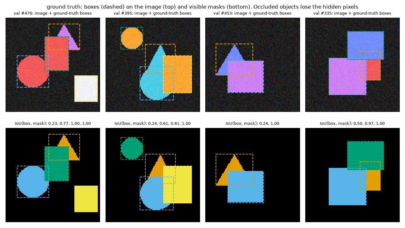
Figure 13-4 shows the two cases where boxes and masks diverge. One is shape: a fully visible circle is around 0.8 and a square is 1.00, exactly the \(\pi/4\) and 1 worked out by hand earlier. The other is occlusion. The triangle in the first image is covered by a square, leaving only its top and right corner, and its box-based IoU is 0.23. The red square in the fourth image is half hidden, giving 0.50. The box is that of the original shape including the hidden part, so it stays the same; only the mask shrinks. Of the 1,265 ground-truth objects in the validation set, 252 are at least partly occluded like this (mean visible fraction 0.899, minimum 0.467).
Training setup and run
The choices made for the experiment, and why:
- Start from the chapter 11 checkpoint. Load the EMA weights from
ch11_rfdetr.pt(the weights that scored 0.9347 box AP in chapter 11) and freshly initialize only the segmentation head. Retraining from scratch would mean repeating about 16 minutes of detection training, and this approach also fits the chapter's theme of "adding one head to a detector." The difference is that the official models learn detection and segmentation together from pre-training onward. - Train everything together, not just the head. The backbone, projector, and decoder are not frozen. The projector output and query embeddings were originally learned for predicting boxes, so this leaves room for them to shift a little toward masks. At the same time, we watch what happens to box AP as a result.
- Everything else is as in chapter 11. AdamW, a 2e-4 learning rate schedule (with layer-wise decay for the backbone), batch 32, gradient clipping at 0.1, EMA (decay 0.993). The segmentation head's learning rate is the default 2e-4.
- 30 epochs, one seed. The main experiment is a single run with seed 0. Only the ablations were run with 3 seeds.
code/ch13_seg.py · train (collapsed in the original)
def seg_targets_to(targets, device):
    """정답 목록(박스 · 클래스 · 마스크)을 장치로 옮긴다. 이어 붙여 한 번에 옮긴 뒤 다시 나눈다."""
    sizes = [len(t["labels"]) for t in targets]
    boxes = torch.cat([t["boxes"] for t in targets]).to(device).split(sizes)
    labels = torch.cat([t["labels"] for t in targets]).to(device).split(sizes)
    masks = torch.cat([t["masks"] for t in targets]).to(device).split(sizes)
    return [{"boxes": b, "labels": c, "masks": m} for b, c, m in zip(boxes, labels, masks)]

def train_one_epoch(model, criterion, loader, optimizer, device, ema: ModelEMA | None = None, max_norm: float = 0.1):
    """한 에폭 학습 (11장과 같은 고리: 기울기 자르기 0.1, 스텝마다 EMA). 돌려주는 값: 손실 이름 → 에폭 평균."""
    model.train()
    criterion.train()
    sums, steps = {}, 0
    for images, targets in loader:
        losses = criterion(model(images.to(device)), seg_targets_to(targets, device))
        optimizer.zero_grad(set_to_none=True)
        losses["loss"].backward()
        nn.utils.clip_grad_norm_(model.parameters(), max_norm)
        optimizer.step()
        if ema is not None:
            ema.update(model)
        for k, v in losses.items():
            sums[k] = sums.get(k, 0.0) + v.detach()
        steps += 1
    return {k: float(v) / steps for k, v in sums.items()}

@torch.no_grad()
def predict_seg(model, dataset, device, batch_size: int = 250, **forward_kwargs):
    """데이터셋 전체를 추론 모드로 순전파 → 후처리한 예측 목록 (CPU). 분할 머리가 없는 모델이면 "masks" 가 없다."""
    model.eval()
    size = dataset.images.shape[-2:]
    predictions = []
    for start in range(0, len(dataset), batch_size):
        images = dataset.images[start:start + batch_size].to(device).float() / 255.0
        outputs = model(images, **forward_kwargs)
        if "pred_masks" in outputs:
            batch_predictions = postprocess_seg(outputs, size)
        else:
            from ch10_rfdetr_model import postprocess
            batch_predictions = postprocess(outputs)
        predictions.extend({k: v.cpu() for k, v in p.items()} for p in batch_predictions)
    return predictions

def evaluate_seg(model, dataset, device, **forward_kwargs):
    """돌려주는 값: (박스 AP 결과, 마스크 AP 결과 또는 None, 예측 목록)."""
    predictions = predict_seg(model, dataset, device, **forward_kwargs)
    box = evaluate_box_ap(predictions, dataset.targets)  # 3장 evaluate_ap 와 같은 값 (check), 더 빠르다
    mask = evaluate_mask_ap(predictions, dataset.targets) if "masks" in predictions[0] else None
    return box, mask, predictions

def build_model(device, seed: int = 0, with_head: bool = True, mask_downsample_ratio: int = 4, verbose: bool = True):
    """ch11_rfdetr.pt 의 EMA 가중치(11장에서 평가에 쓴 가중치)에서 출발하는 모델. 분할 머리만 새로 초기화된다.

    체크포인트가 없으면 전부 무작위 초기화. 돌려주는 값: (모델, 체크포인트를 실었는지).
    """
    torch.manual_seed(seed)
    config, state = {}, None
    if os.path.exists(CHECKPOINT_IN):
        checkpoint = torch.load(CHECKPOINT_IN, map_location="cpu")
        config, state = checkpoint["config"], checkpoint["ema"]
    model = MiniRFDETRSeg(mask_downsample_ratio, **config) if with_head else MiniRFDETR(**config)
    if state is not None:
        missing, unexpected = model.load_state_dict(state, strict=False)
        assert not unexpected and all(k.startswith("segmentation_head.") for k in missing)
        if verbose:
            print(f"  {CHECKPOINT_IN} 의 EMA 가중치를 실었다. 새로 초기화된 텐서 {len(missing)}개 (모두 segmentation_head.*)")
    elif verbose:
        print(f"  ({CHECKPOINT_IN} 가 없어 무작위 초기화에서 시작한다 — 11장을 먼저 돌리면 거기서 이어 학습한다)")
    return model.to(device), state is not None

def fit(model, criterion, optimizer, loader, val_set, epochs: int, device, ema: ModelEMA, verbose: bool = True):
    """epochs 에폭 학습하며 에폭마다 EMA 모델을 채점한다. 돌려주는 값: 기록 사전 (에폭 0 = 학습 전)."""
    keys = ("epoch", "loss", "loss_ce", "loss_bbox", "loss_giou", "loss_maskce", "loss_maskdice", "time",
            "box_AP", "mask_AP", "mask_AP50", "mask_AP75")
    history = {k: [] for k in keys}
    box, mask, _ = evaluate_seg(ema.module, val_set, device)
    history["epoch"].append(0)
    history["box_AP"].append(box["AP"])
    for k in ("AP", "AP50", "AP75"):
        history["mask_" + k].append(mask[k] if mask else float("nan"))
    if verbose:
        print(f"에폭   0 | (학습 전) 박스 AP {box['AP']:.4f}" + (f" | 마스크 AP {mask['AP']:.4f}" if mask else ""))
    start = time.time()
    for epoch in range(1, epochs + 1):
        losses = train_one_epoch(model, criterion, loader, optimizer, device, ema)
        history["epoch"].append(epoch)
        history["time"].append(time.time() - start)
        for k in keys[1:7]:
            history[k].append(losses.get(k, float("nan")))
        box, mask, _ = evaluate_seg(ema.module, val_set, device)
        history["box_AP"].append(box["AP"])
        for k in ("AP", "AP50", "AP75"):
            history["mask_" + k].append(mask[k] if mask else float("nan"))
        if verbose:
            text = (f"maskce {losses['loss_maskce']:.4f} maskdice {losses['loss_maskdice']:.4f}) | 박스 AP {box['AP']:.4f} | "
                    f"마스크 AP {mask['AP']:.4f} AP50 {mask['AP50']:.4f} AP75 {mask['AP75']:.4f}" if mask else
                    f") | 박스 AP {box['AP']:.4f}")
            print(f"에폭 {epoch:3d} | 손실 {losses['loss']:7.4f} (ce {losses['loss_ce']:.4f} bbox {losses['loss_bbox']:.4f} "
                  f"giou {losses['loss_giou']:.4f} {text} | {time.time() - start:4.0f}초", flush=True)
    return history

def run_experiment(name, train_set, val_set, epochs, device, seed: int = 0, with_head: bool = True,
                   mask_downsample_ratio: int = 4, batch_size: int = 32, lr: float = 2e-4, verbose: bool = True,
                   **criterion_kwargs):
    """모델(체크포인트에서) · 손실 · 옵티마이저 · EMA 를 만들어 학습한다. 돌려주는 값: (model, ema, history).

    옵티마이저는 11장 build_optimizer 그대로다 (분할 머리는 "그 밖" 그룹: 기본 학습률 2e-4, 감쇠 없음).
    """
    print(f"\n[{name}]")
    model, _ = build_model(device, seed, with_head, mask_downsample_ratio, verbose)
    if with_head:
        criterion = SegCriterion(NUM_CLASSES, group_detr=model.group_detr, **criterion_kwargs).to(device)
    else:
        criterion = RFDETRCriterion(NUM_CLASSES, group_detr=model.group_detr).to(device)
    optimizer, _ = build_optimizer(model, lr)
    ema = ModelEMA(model)
    loader = make_loader(train_set, batch_size, shuffle=True, seed=seed)
    if verbose:
        head = sum(p.numel() for p in model.segmentation_head.parameters()) if with_head else 0
        print(f"  매개변수 {sum(p.numel() for p in model.parameters()):,}개 (분할 머리 {head:,}개), 에폭 {epochs}, "
              f"에폭당 {len(loader)} 스텝, 학습 그림 {len(train_set)}장")
    history = fit(model, criterion, optimizer, loader, val_set, epochs, device, ema, verbose)
    return model, ema, history
The first part of the output (hand calculations and checks) was shown earlier. The training part follows.
[미니 RF-DETR-Seg (본 실험): BCE + 다이스, 점 표본 추출, 마스크 1/4 해상도]
  ch11_rfdetr.pt 의 EMA 가중치를 실었다. 새로 초기화된 텐서 29개 (모두 segmentation_head.*)
  매개변수 2,051,844개 (분할 머리 219,137개), 에폭 30, 에폭당 125 스텝, 학습 그림 4000장
에폭   0 | (학습 전) 박스 AP 0.9347 | 마스크 AP 0.0028
에폭   1 | 손실 13.4178 (ce 0.2578 bbox 0.0160 giou 0.0522 maskce 0.2413 maskdice 0.2870) | 박스 AP 0.8906 | 마스크 AP 0.4748 AP50 0.8007 AP75 0.5072 |   21초
에폭   2 | 손실  8.7491 (ce 0.2600 bbox 0.0176 giou 0.0569 maskce 0.1190 maskdice 0.1527) | 박스 AP 0.8914 | 마스크 AP 0.6361 AP50 0.9255 AP75 0.7108 |   50초
에폭   3 | 손실  7.1792 (ce 0.2570 bbox 0.0177 giou 0.0571 maskce 0.0916 maskdice 0.1127) | 박스 AP 0.9032 | 마스크 AP 0.6987 AP50 0.9610 AP75 0.7928 |   81초
에폭   4 | 손실  6.1754 (ce 0.2440 bbox 0.0170 giou 0.0551 maskce 0.0737 maskdice 0.0917) | 박스 AP 0.9077 | 마스크 AP 0.7384 AP50 0.9708 AP75 0.8255 |   95초
에폭   5 | 손실  5.4888 (ce 0.2332 bbox 0.0166 giou 0.0535 maskce 0.0624 maskdice 0.0785) | 박스 AP 0.9093 | 마스크 AP 0.7581 AP50 0.9709 AP75 0.8419 |  112초
  …
에폭  10 | 손실  3.9809 (ce 0.1947 bbox 0.0143 giou 0.0467 maskce 0.0402 maskdice 0.0544) | 박스 AP 0.9198 | 마스크 AP 0.8254 AP50 0.9727 AP75 0.9006 |  184초
  …
에폭  15 | 손실  3.3326 (ce 0.1711 bbox 0.0123 giou 0.0411 maskce 0.0328 maskdice 0.0448) | 박스 AP 0.9289 | 마스크 AP 0.8546 AP50 0.9797 AP75 0.9152 |  282초
  …
에폭  20 | 손실  2.9818 (ce 0.1561 bbox 0.0110 giou 0.0371 maskce 0.0295 maskdice 0.0415) | 박스 AP 0.9325 | 마스크 AP 0.8631 AP50 0.9769 AP75 0.9079 |  374초
  …
에폭  25 | 손실  2.7625 (ce 0.1477 bbox 0.0101 giou 0.0344 maskce 0.0266 maskdice 0.0391) | 박스 AP 0.9344 | 마스크 AP 0.8702 AP50 0.9840 AP75 0.9154 |  471초
  …
에폭  30 | 손실  2.6449 (ce 0.1428 bbox 0.0096 giou 0.0329 maskce 0.0256 maskdice 0.0386) | 박스 AP 0.9349 | 마스크 AP 0.8766 AP50 0.9884 AP75 0.9176 |  562초
저장: ch13_seg.pt (model · ema · config · history). 학습 561초 (3750 스텝)
On a single laptop GPU, training took 561 seconds and the full run including analysis 582 seconds (measured while sharing the GPU with other work). The values in parentheses on each line are the losses of the last decoder layer (before multiplying by the coefficients), and AP is the EMA model scored on the validation set. The middle epochs are omitted.
Re-running only the analysis. After training, ch13_seg.pt is left in the working directory. The tables and figures that follow can be regenerated without training with python ch13_seg.py --analyze (about 35 seconds). Use it to redraw figures or look at other validation images. The figures in this chapter were redrawn that way, and the numbers in the tables matched the output right after training character for character.
Reading the training log
- Figure 13-5: ch13-curves.png Left: training losses (last decoder layer, log-scale vertical axis). Right: validation AP. Epoch 0 is right after the segmentation head is attached, before training. The gray dashed line is the box AP of the chapter 11 model.
- (Figure content) Left: mask BCE, mask Dice, classification, and GIoU losses over epochs. Right: validation box AP and mask AP. Mask AP rises quickly from 0, while box AP drops at first and then returns to its original level.
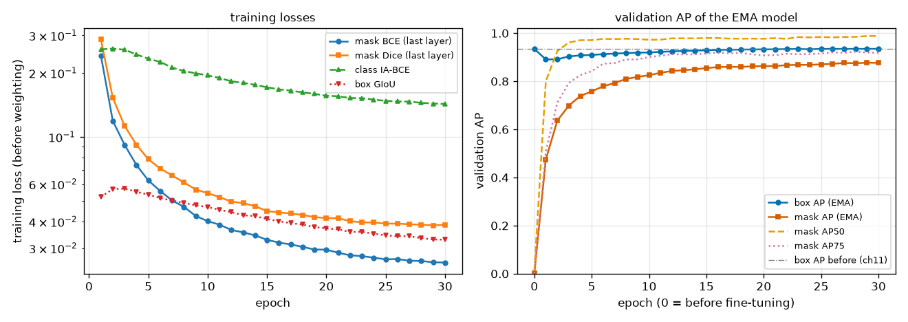
Four things can be read from figure 13-5 and the output above.
- Masks are learned quickly. Mask AP reaches 0.4748 after one epoch, 0.7581 after five, and 0.8766 after 30. The detector already knows how to find objects, and the projector output already contains object locations, so the head only has to learn to turn that into masks. The chapter 11 detector, trained from scratch, had a box AP of 0.31 after one epoch.
- AP at low thresholds fills in first, high thresholds later. Mask AP50 passes 0.96 by epoch three and is nearly saturated, while AP75 is 0.79 at that point and keeps creeping up to the end. The rough region is captured quickly; refining the boundary takes time.
- Box AP drops at first. It falls from 0.9347 to 0.8906 after one epoch, then slowly recovers to 0.9349 at epoch 30. At the end it is effectively the same as chapter 11 (a difference of 0.0002). Attaching the segmentation head neither improved nor hurt the boxes. Whether the drop was caused by the mask loss cannot be told from this curve alone; it is examined with the control group in the ablations.
- The two mask losses fall together. BCE goes from 0.24 to 0.026, and Dice from 0.29 to 0.039. Even at epoch 30 they have not completely flattened.
Box AP and mask AP
[최종] EMA 모델, 검증 500장
  박스 AP 0.9349 AP50 0.9926 AP75 0.9797  (학습 전 0.9347)
  마스크 AP 0.8766 AP50 0.9884 AP75 0.9176
  클래스별 박스 AP: circle 0.9685, rectangle 0.9068, triangle 0.9294
  클래스별 마스크 AP: circle 0.9016, rectangle 0.9083, triangle 0.8199
  IoU 문턱값별 AP (클래스 평균):
    문턱값  | 0.50 | 0.55 | 0.60 | 0.65 | 0.70 | 0.75 | 0.80 | 0.85 | 0.90 | 0.95
    박스    | 0.99 | 0.99 | 0.99 | 0.99 | 0.99 | 0.98 | 0.97 | 0.94 | 0.89 | 0.62
    마스크  | 0.99 | 0.97 | 0.95 | 0.94 | 0.93 | 0.92 | 0.90 | 0.86 | 0.79 | 0.52
  기준선 (정답 마스크를 24×24 로 줄였다가 되키운 것을 예측으로): 마스크 AP 0.9266 AP50 1.0000 AP75 1.0000
Mask AP is 0.8766, about 0.06 below the box AP of 0.9349. The per-threshold lines show where the gap opens. At IoU 0.50 the two are equal (0.99); at 0.75 it is 0.98 vs 0.92, at 0.90 0.89 vs 0.79, and at 0.95 0.62 vs 0.52. The model produces "roughly right masks" as well as boxes, but "nearly perfect masks" are harder than boxes.
By class, the gap is uneven. For rectangles, mask AP (0.9083) is on par with box AP (0.9068); for circles it is 0.9016 vs 0.9685; and for triangles 0.8199 vs 0.9294, the widest gap. A triangle's sharp apex and slanted sides are the hardest shape to draw on a 24×24 grid with 4-pixel spacing.
The baseline on the last line was added to gauge the limit of this resolution. The ground-truth masks were downsampled to 24×24 (averaging area per cell), upsampled back to 96×96, thresholded at 0.5, and fed in as the masks of perfect detections with score 1. Even with every object found and every class right, the mask AP is 0.9266. AP50 and AP75 are 1.0, so everything lost is at thresholds above 0.75. The mini model's 0.8766 is 0.05 below this baseline. This baseline is not a strict upper bound, though: the model upsamples logits before thresholding, so it can place the boundary anywhere between cells and could in principle do better.
Looking at predicted masks
- Figure 13-6: ch13-predictions.png The first six images of the validation set. Top: the image; middle: ground-truth masks; bottom: masks (color) and boxes (dashed) of predictions with score 0.5 or higher. Colors are only for telling objects apart, and ground truth and predictions need not share colors. The IoU in the bottom-row titles is the mask IoU with the best-overlapping prediction, averaged over ground-truth objects.
- (Figure content) Six validation images. Top row: images; middle row: ground-truth masks; bottom row: predicted masks and predicted boxes. Most are nearly identical to the ground truth; in one image the same circle has two predictions, and in another a rectangle is missing.
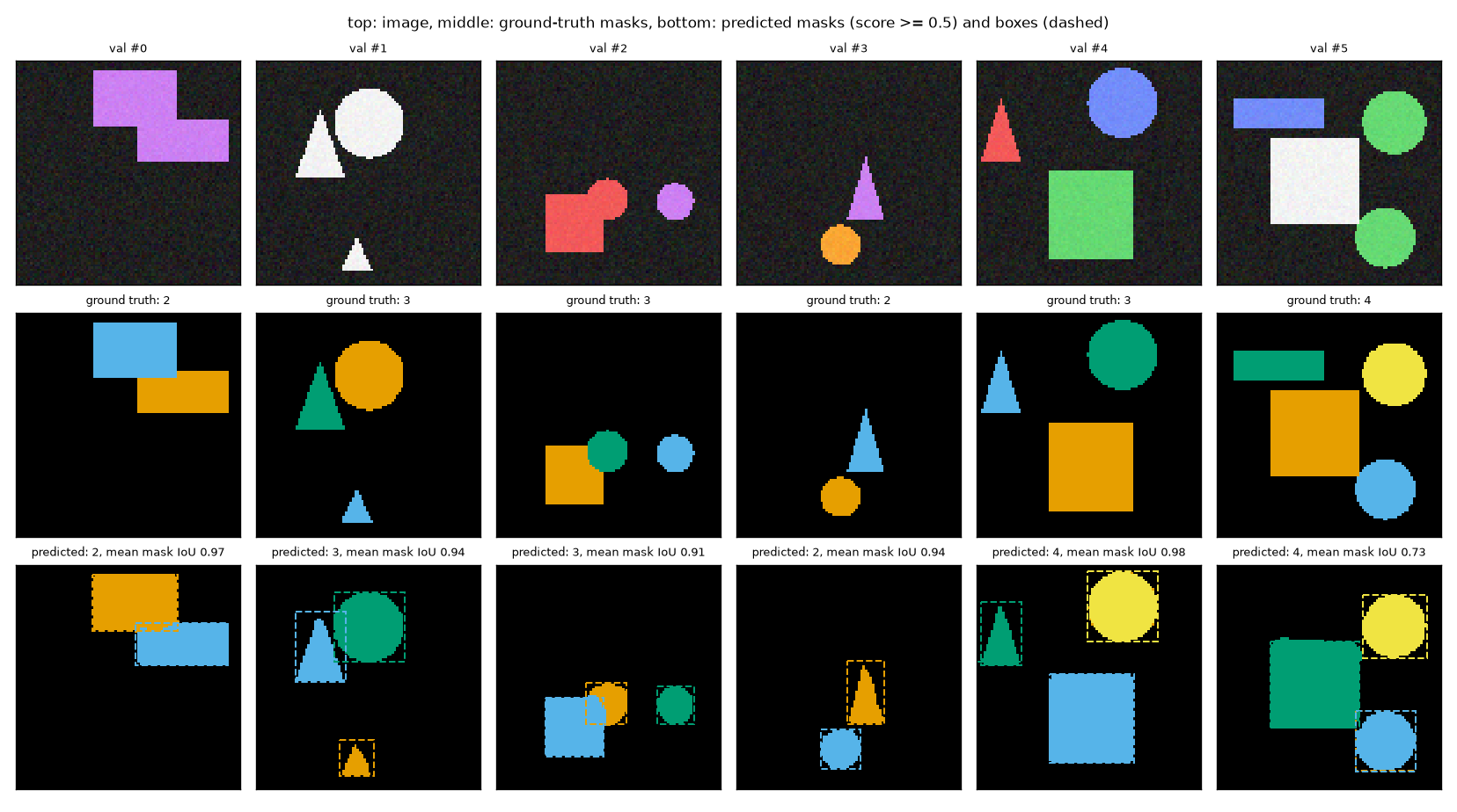
Compare the bottom row of figure 13-6 with the middle row. The round edges of circles and the slanted sides of triangles are drawn true to shape, unlike the boxes (dashed). The two touching rectangles in #0 and the small circle overlapping a rectangle's corner in #2 also come out as separate masks. There are two errors. #4 has three ground-truth objects but four predictions: two predictions are attached to the upper circle (both with accurate masks), and one is painted over the other, so they look like one in the figure. #5 is missing the flat rectangle at the top left. There is a query that draws that rectangle with an accurate mask, but its class score falls short of 0.5, so it does not appear in the figure. Instead, two predictions are attached to the circle at the bottom right. In both cases the problem lies not in the mask but in the classification score. Mask quality and the judgment "is this query an object" are handled by different heads.
The dot-product map of a single query
- Figure 13-7: ch13-dot-product.png Validation image #7 (four objects). The top row is the logit map from the dot product of one query's \(f(q_n)\) with every 24×24 pixel embedding (red = positive, blue = negative, black line = 0). The bottom row shows the outline (green) of the mask obtained by upsampling those logits to 96×96 and thresholding at 0. The four on the left are high-scoring queries; the rightmost is the lowest-scoring query.
- (Figure content) Mask logit maps (24×24) for five queries on one image, and the masks obtained by upsampling and thresholding them. The four high-scoring queries are each positive on only one object, and even the query with a score of 0 draws a circle cleanly.
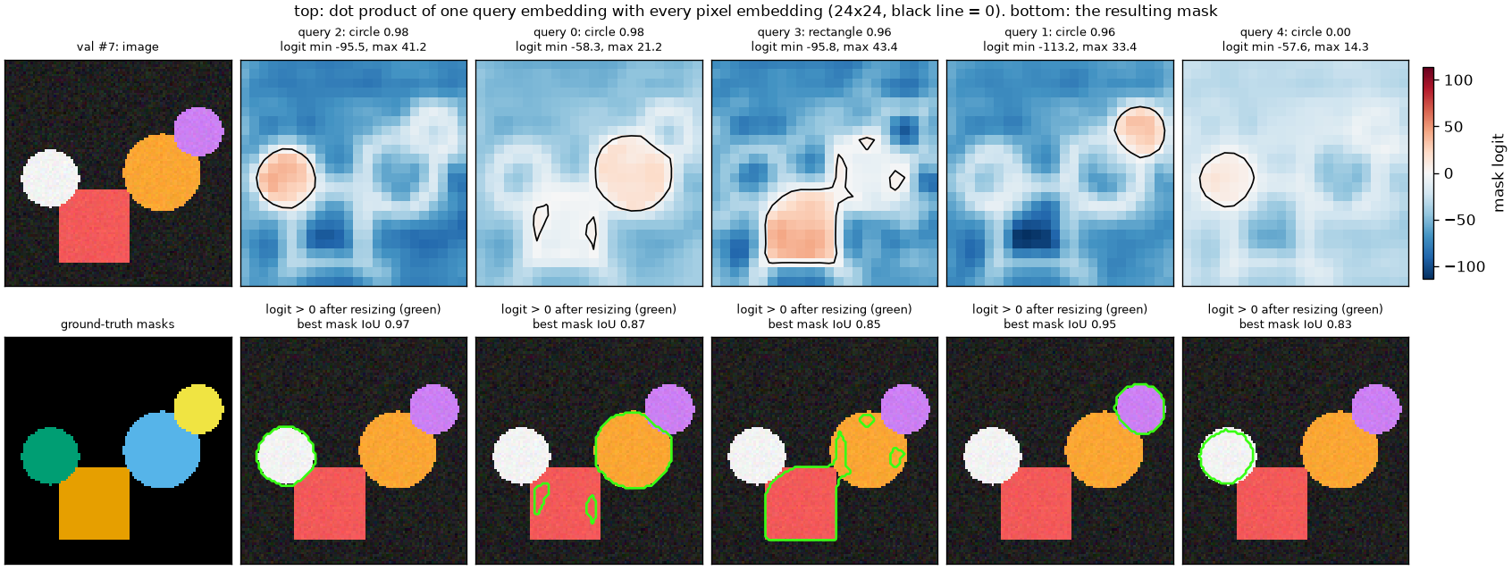
Figure 13-7 is a direct picture of this chapter's formula \(z_n(x, y) = \langle f(q_n), e(x, y) \rangle + \beta\).
- Each query is positive on a different object. The pixel embedding map is the same single map in all five columns. Only the query-side vector changes, yet the positive region switches between the white circle, the orange circle, the rectangle, and the purple circle.
- The logits are large in magnitude. The minimum is around \(-113\) and the maximum around \(43\). After the sigmoid, most cells stick to 0 or 1, and the model hesitates only on a cell or two at the boundary. This shows why it is useful for point sampling to pick "points with logits near 0."
- Other objects' outlines show through. In every query's map, the outlines of all four objects appear as faint bands, because all queries share the pixel embeddings. These usually stay negative but sometimes leak through. In the second column (orange circle), two small blobs inside the rectangle cross 0, and in the third column (rectangle), a part sticking out toward the orange circle does. That is why their mask IoUs, 0.87 and 0.85, are lower than the other two (0.97, 0.95).
- Even a query with a score of 0 draws a mask. The rightmost query has a class score of 0.00 but draws the white circle with an IoU of 0.83. This is not strange. The mask loss applies only to queries matched to ground truth, so the masks of unmatched queries are not penalized whatever their shape. This query drops out of the predictions not because of its mask but because the classification head gives it a low score.
Looking inside the pixel embeddings
The pixel embedding map has 128 numbers per cell, so it cannot be viewed directly. Two approaches are used. One is principal component analysis (PCA), which reduces the 128 dimensions to the three directions of greatest variation and maps them to red, green, and blue (the method used to view DINOv2 features in chapter 6); the other is to look at a few channels directly.
- Figure 13-8: ch13-pixel-embedding.png Top: images. Bottom: their pixel embedding maps (24×24, 128 channels) reduced to three principal components and shown as color. Cells with similar colors have similar embeddings. The 2,880 cells of all five images were analyzed together, so colors can be compared across images.
- (Figure content) Five validation images and the three principal components of their pixel embedding maps shown as color. The background is pink and orange, objects are green or blue, and there is a dark purple band around each object.
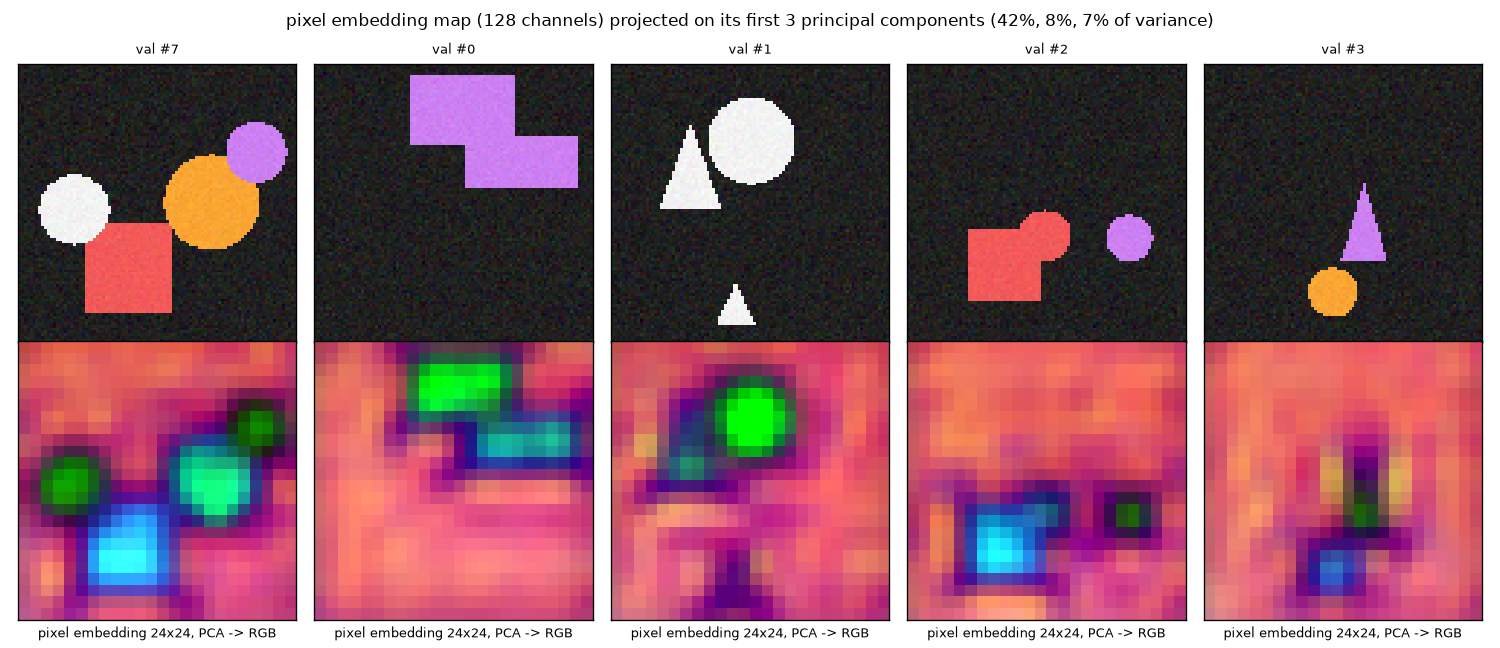
Three things are visible in figure 13-8. First, objects and background separate. The background is in pinks and oranges, while objects are green or blue. Second, there is a dark band around each object: cells near the boundary have embeddings different from both the interior and the background. Third, each object has a different color. The rectangle in #7 is sky blue, and the three circles are greens of different brightness. But color does not indicate class: the circle in #3 is blue, and the two rectangles in #0 differ, green and teal. To pick out a single object by dot product, its embedding must also differ from other objects of the same class, so separating only by class would actually be a problem. The background is not a single color either, but varies slightly with position.
[픽셀 임베딩] 검증 그림 5장의 픽셀 임베딩 (5·24·24 = 2,880개, 128차원): 주성분 분산 비율 0.423, 0.083, 0.075, 0.063, 0.046, 0.039, 앞 3개 합 0.581, 앞 10개 합 0.822
  분산이 큰 채널 8개: [1, 63, 54, 32, 6, 111, 124, 75]. 그림에 쓴 검증 그림: #7 (객체 4개), #0 – #3
Looking at the variance ratios of the principal components, the single largest direction among the 128 channels accounts for 42% of the variance, and the first ten for 82%. There are 128 channels, but far fewer directions are actually used. This echoes the YOLACT paper's finding that 32 prototypes were enough (with only three shape types in a small world, this experiment probably needs even fewer directions).
- Figure 13-9: ch13-prototypes.png The eight highest-variance channels of the pixel embedding map (red = positive, blue = negative). Each channel is one prototype. The rows are validation images #7, #0, and #1.
- (Figure content) Eight channels of the pixel embedding map drawn directly for three validation images. Some channels are positive on the background and negative on objects, and some respond strongly only on certain objects.
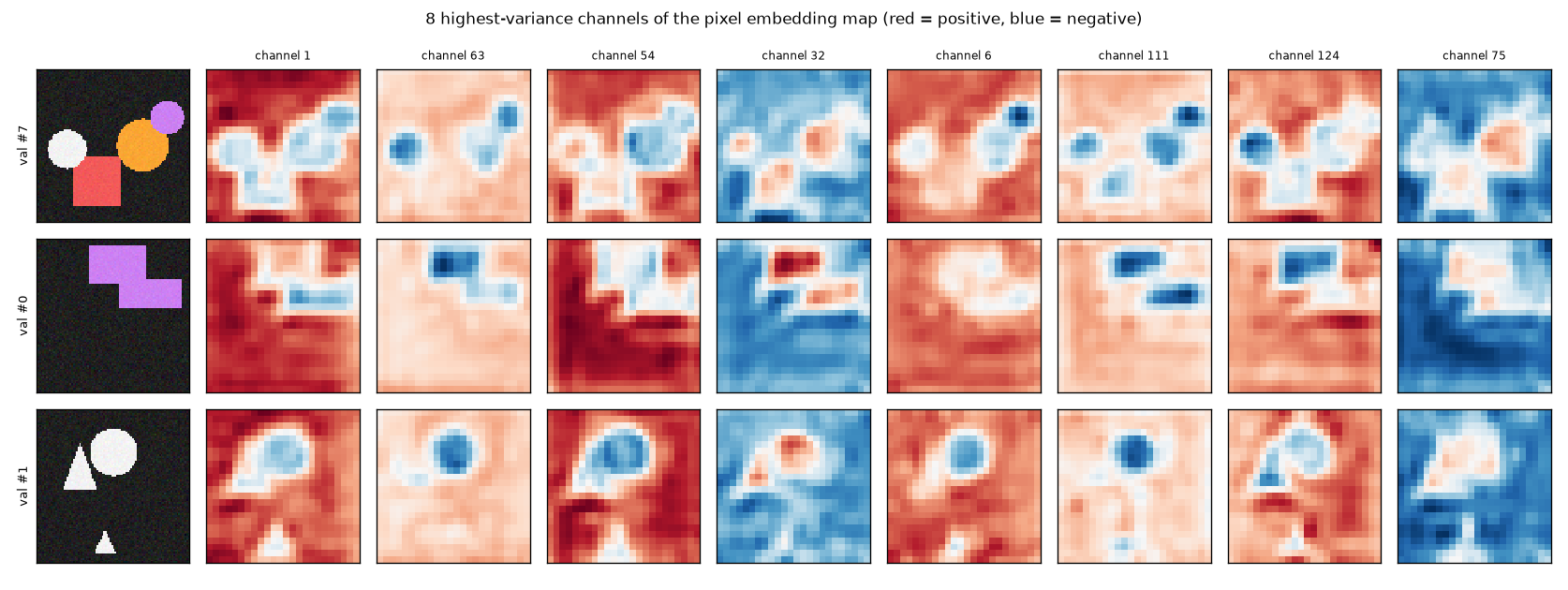
Figure 13-9 is what "prototypes" actually look like. No channel cleanly cuts out a single object. Channels 1 and 54 have a "background vs object" pattern, positive on the background and negative where objects are; channels 63 and 111 are strongly negative only on some objects. Channel 32 is the reverse, negative on the background and positive inside objects. Masks are built by adding and subtracting these 128 patterns with different coefficients for each query. This shows why the YOLACT paper stressed that coefficients must be able to be negative (that prototypes must be subtractable): no single map separates an object, and only by subtracting one map from another is a single object left.
Dropping decoder layers
The paper said that reducing the decoder also shrinks the segmentation branch. The trained model was scored at inference with only \(k\) decoder layers (dec_layers=k), using the same weights without retraining.
[디코더 층 수별] dec_layers = k 로 추론 (k 층만 쓰면 분할 머리의 블록도 k 개만 쓰인다; 0 = 인코더 제안, 블록 없음)
  층 수 | 박스 AP | 마스크 AP | 마스크 AP50 | 마스크 AP75 | 마스크 IoU 평균
      0 | 0.8787  | 0.7863    | 0.9657      | 0.8553      | 0.8838
      1 | 0.9233  | 0.8429    | 0.9732      | 0.8882      | 0.9068
      2 | 0.9325  | 0.8748    | 0.9844      | 0.9247      | 0.9236
      3 | 0.9349  | 0.8766    | 0.9884      | 0.9176      | 0.9274
- Figure 13-10: ch13-layers.png Left: validation metrics by the number of decoder layers used at inference. Right: predicted masks (score 0.5 or higher) for validation image #7 at each layer count. Layer 0 is the prediction from encoder proposals alone, which passes through none of the segmentation head's blocks.
- (Figure content) Left: box AP, mask AP, and mean mask IoU for 0 to 3 decoder layers. They rise as layers are added and are nearly flat from 2 layers on. Right: predicted masks for the same image at each layer count. At 0 layers, other masks are mixed into the rectangle, and they get cleaner as layers are added.
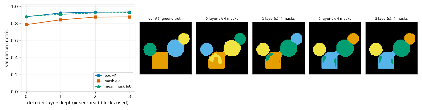
What to read from figure 13-10 and the table:
- Dropping the last layer costs almost nothing. Going from 3 layers to 2, mask AP falls from 0.8766 to 0.8748 and box AP from 0.9349 to 0.9325. AP75 is actually higher with 2 layers (0.9247 vs 0.9176). Differences this small cannot be distinguished from chance.
- Masks are more sensitive to layer count than boxes. Going from 3 layers to 0, box AP drops 0.056 and mask AP 0.090. With 0 layers there is no decoder and no block; the pixel embedding is just the interpolated projector output after a 1×1 convolution. Adding one decoder layer and one block raises mask AP by 0.057.
- Still, 0 layers gives 0.79. That masks passing through no block at all are usable means most of the information needed for masks is already in the projector output. In the right panel, the 0-layer masks are in the right places, but other queries' masks are mixed into the rectangle, and such blotches decrease as layers are added.
Regarding the segmentation models' decoders being deeper than the detection models' (even the smallest has 4 layers), the paper suggested there seems to be "a minimum depth for a usable segmentation head." This experiment points the same way, with masks depending more on layer count. However, this mini model needed only 2 layers, and the experiment says nothing about how many layers the complex shapes of COCO require.
Box IoU and mask IoU
Back to this chapter's opening question: how much better does a mask represent an object's region than a box? For each ground-truth object, the prediction that found it (same class, score 0.5 or higher, highest mask IoU) was selected and four things were measured.
- Mask IoU when the ground-truth box itself is used as the region (the limit when the box is perfect)
- Mask IoU when the predicted box is used as the region (what a detector alone gives)
- Mask IoU of the predicted mask (what the segmentation head adds)
- Mask IoU of the ground-truth mask downsampled to 1/4 resolution and upsampled back (the baseline from earlier)
[객체별 분석] 정답 객체 1265개 가운데 점수 ≥ 0.5 · 같은 클래스 · 겹치는 예측이 있는 것 1259개. 마스크 IoU 평균 0.9274 (찾은 것만 0.9318), 박스 IoU 평균 0.9415
  클래스      | 객체 수 | 정답 박스를 마스크로 | 예측 박스를 마스크로 | 예측 마스크 | 박스 IoU | 1/4 기준선 | 1/2 기준선
  circle      |     428 |               0.7696 |               0.7564 |      0.9300 |   0.9549 |     0.9611 |     0.9895
  rectangle   |     445 |               0.9774 |               0.9538 |      0.9452 |   0.9295 |     0.9722 |     0.9940
  triangle    |     392 |               0.4913 |               0.4843 |      0.9043 |   0.9404 |     0.9151 |     0.9751
  보이는 넓이(픽셀) | 객체 수 | 예측 마스크 IoU | 박스 IoU | 1/4 기준선 | 1/2 기준선
  0 – 300           |     305 |          0.8792 |   0.9094 |     0.9090 |     0.9743
  300 – 700         |     607 |          0.9299 |   0.9436 |     0.9550 |     0.9881
  700 이상            |     353 |          0.9647 |   0.9655 |     0.9795 |     0.9947
  가림 (보이는 비율)            | 객체 수 | 예측 마스크 IoU | 박스 IoU | 정답 박스를 마스크로 | 예측 박스를 마스크로
  가려지지 않음 (1.0)          |    1013 |          0.9393 |   0.9525 |               0.7640 |               0.7518
  조금 가려짐 (0.9 이상)        |     161 |          0.9261 |   0.9417 |               0.7744 |               0.7595
  많이 가려짐 (0.9 미만)        |      91 |          0.7973 |   0.8189 |               0.6407 |               0.5955
  가려진 객체 252개의 보이는 비율: 평균 0.899, 최소 0.467
- Figure 13-11: ch13-iou-by-class.png Mean IoU with the ground-truth mask, by class. Gray uses the ground-truth box as the region, blue hatching uses the predicted box, orange is the predicted mask, and green dots are the 1/4-resolution baseline.
- (Figure content) Bar chart by class. For circles and triangles, the predicted mask's IoU is far higher than using the box as the region; for rectangles, all four are similar.
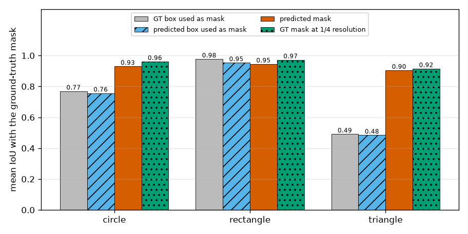
- Masks win by a wide margin on triangles and circles. For triangles, using the box as the region gives 0.48, while the mask gives 0.90. For circles it is 0.76 vs 0.93. The gray bars (0.49, 0.77) are the 0.5 and \(\pi/4 \approx 0.785\) worked out by hand earlier, lowered by occlusion and the pixel grid.
- On rectangles, the box slightly beats the mask. Using the predicted box as the region gives 0.9538, and the predicted mask 0.9452. For a rectangle the box is the shape, and with four real-valued coordinates a box can place its sides more finely than pixels. A mask is upsampled from a 24×24 grid, so its corners get rounded. The segmentation head is not always better than the box.
- The smaller the object, the worse the mask. Objects with a visible area under 300 pixels have a mask IoU of 0.879, and those over 700 pixels 0.965. The baseline goes the same way (0.909 vs 0.980). A 300-pixel object covers about 19 cells on the 24×24 grid, and a handful of cells cannot draw a precise boundary. This is the same phenomenon as APS depending most on input resolution in the paper's table.
- At 1/2 resolution. The last baseline column is for a 48×48 mask grid. The baseline for small objects rises from 0.909 to 0.974. Whether the model actually improves that much is checked in the ablations.
On overlapping objects
The last table in the output above splits objects by how occluded they are. Mask IoU is 0.939 for unoccluded objects and 0.926 for slightly occluded ones (visible fraction 0.9 or more), nearly the same, but drops sharply to 0.797 for heavily occluded objects (below 0.9, 91 objects). Box IoU falls with it, to 0.819. Still, the mask beats the box: for heavily occluded objects, using the predicted box as the region gives 0.596, so the mask is 0.2 higher. That is about the same size as the gap for unoccluded objects (0.939 vs 0.752).
- Figure 13-12: ch13-overlap.png Among objects with a visible fraction below 0.9, the four with the highest mask IoU (top) and the four with the lowest (bottom). The white dashed line is that object's ground-truth mask, and the green solid lines are all predicted masks in that image (score 0.5 or higher).
- (Figure content) Eight heavily occluded objects. In the top four, the masks accurately follow the shape minus the hidden part; in the bottom four, the object has merged with a neighboring shape of the same color, or there is no prediction.
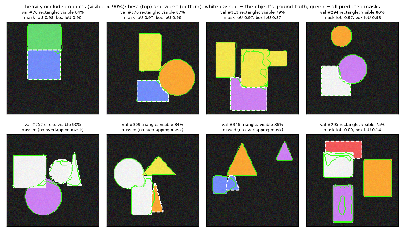
The top row of figure 13-12 shows successes. Rectangles partly covered by other shapes are drawn in the shape that remains after removing the covered part (an L shape, or a shape with a rounded bite taken out of a corner), shapes a box cannot represent. The bottom row shows failures. For the first three, no prediction overlaps the object at all ("missed" in the titles). Two of them are cases where shapes of the same color touch: in #252 a white circle is attached to a white rectangle and a white triangle, and in #346 a blue triangle is attached to a blue rectangle. With no color boundary to go on, the model extended the neighboring shape's mask over that area. The orange triangle in #309 was missed even though its color is different. The fourth (#295) is a red rectangle whose lower part is hidden by a white rectangle, leaving only a long horizontal strip, and no mask draws that strip properly. These four are detection failures before they are segmentation-head failures: if no query finds the object, there is no mask either.
Occlusion in the shapes world is mild. When generating scenes, the shapes world prevents two shapes' boxes from overlapping by more than 35% of the smaller one's area (max_covered in rf_shapes.py). So even the most occluded object in the validation set is nearly half visible (0.467). Cases where most of an object is hidden, as in a photo of a dense crowd, do not occur in this experiment.
The cost of the segmentation head
[분할 머리의 값] 매개변수 219,137 / 2,051,844 (10.7%). 추론 순전파 (배치 64, 그림 한 장당, 30번 가운데 최솟값): 분할 머리 없이 0.173 ms, 있을 때 0.258 ms, 모든 층의 마스크까지 0.286 ms
본 실험 전체 582초
In the mini model the segmentation head is 10.7% of the parameters. This is much larger than Nano's 2.8% because the mini model's backbone is small (the head's size is set by \(D\) and does not depend on the backbone). Inference time went from 0.173 ms to 0.258 ms per image, about 1.5×. These are reference values measured on a laptop GPU with PyTorch at batch 64, and as noted in chapter 10, the time of such a small model is governed more by the number of operation calls than by the amount of computation. Comparing two similarly sized models in the paper, RF-DETR (nano) takes 2.3 ms and RF-DETR-Seg (nano) 3.4 ms. However, the two differ in resolution, patch, decoder layer count, and query count, so that difference is not the cost of the segmentation head alone.
Ablations
Finally, the design choices are changed one at a time. Every variant starts from the chapter 11 checkpoint, just like the main experiment, and trains for only 4 epochs. The first row has the same settings as the main experiment, and each other row changes one thing from it. Three seeds (0, 1, 2) were run.
- BCE only (Dice coefficient 0) / Dice only (BCE coefficient 0). The corresponding term in the matching cost also becomes 0.
- Computing the loss over all pixels of the ground-truth mask (9,216) instead of point sampling
- Removing the mask terms from the matching cost (loss unchanged)
- Mask grid at 1/2 (48×48) instead of 1/4 (24×24)
- No segmentation head, training the same 4 extra epochs with the detection loss only (control group for box AP)
$ python ch13_seg.py --ablations            # 시드 0
$ python ch13_seg.py --ablations --seed 1   # 시드 1, 2 도 같은 방법으로
The seven variants are trained in sequence, so each seed takes a little over 8 minutes (500 seconds). At the end, the results for all seeds saved so far are collected into a summary table.
[절제 요약] 4 에폭 뒤의 EMA 모델, 시드 [0, 1, 2] (3개). 평균 (최소 – 최대)
  변형                                       | 박스 AP                  | 마스크 AP                | 마스크 AP75              | 마스크 IoU 평균
  BCE + Dice, uncertain points (official)  | 0.9073 (0.9066 – 0.9085) | 0.7427 (0.7369 – 0.7533) | 0.8359 (0.8226 – 0.8612) | 0.8537 (0.8509 – 0.8559)
  BCE only                                 | 0.9218 (0.9207 – 0.9232) | 0.7074 (0.7043 – 0.7101) | 0.7861 (0.7820 – 0.7888) | 0.8485 (0.8447 – 0.8518)
  Dice only                                | 0.9206 (0.9195 – 0.9227) | 0.5607 (0.5235 – 0.5820) | 0.5900 (0.5375 – 0.6215) | 0.7983 (0.7822 – 0.8074)
  BCE + Dice, all pixels                   | 0.9166 (0.9157 – 0.9174) | 0.7325 (0.7209 – 0.7424) | 0.8163 (0.7975 – 0.8338) | 0.8542 (0.8498 – 0.8579)
  BCE + Dice, no mask term in matching     | 0.9067 (0.9059 – 0.9080) | 0.7394 (0.7338 – 0.7443) | 0.8351 (0.8242 – 0.8533) | 0.8531 (0.8518 – 0.8552)
  BCE + Dice, masks at 1/2 resolution      | 0.9057 (0.9039 – 0.9079) | 0.7747 (0.7677 – 0.7808) | 0.8528 (0.8434 – 0.8666) | 0.8666 (0.8660 – 0.8676)
  no segmentation head (detection only)    | 0.9342 (0.9335 – 0.9354) | —                        | —                        | —
절제 실험 전체 500초
- Figure 13-13: ch13-ablation.png Ablations: validation mask AP (left) and box AP (right) of the EMA model after 4 epochs. Bars are the mean over 3 seeds, and black dots are individual seeds. The horizontal axis does not start at 0.
- (Figure content) Horizontal bar charts of the ablations. Mask AP on the left, box AP on the right. Each variant has a seed-mean bar and per-seed dots.
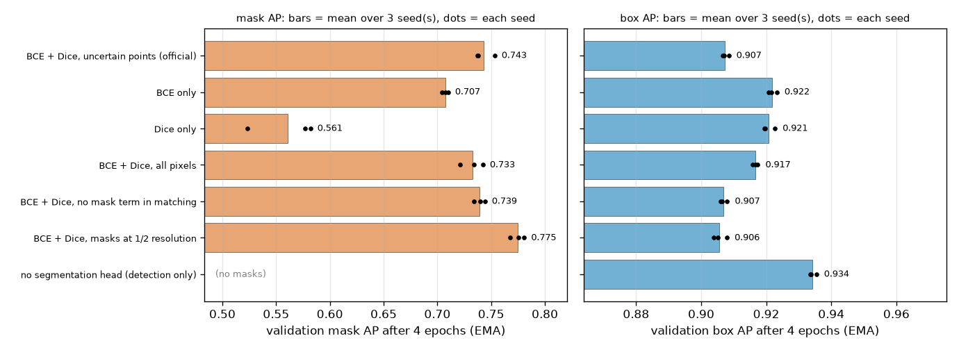
First, a rule for reading the table: the values in parentheses are the minimum–maximum over 3 seeds. If two variants' ranges overlap, the difference is not interpreted.
- BCE and Dice together is best, Dice alone is worst. Mask AP is 0.743 for both, 0.707 for BCE only, and 0.561 for Dice only, with none of the three ranges overlapping. The Dice-only model's mean mask IoU, 0.798, is not terrible, but its AP75 is low at 0.590: it captures the rough region but the boundaries are blunt. This is what the gradient derivation predicted. Dice loss does not distinguish how wrong individual points are, so its signal for refining boundaries cell by cell is weak. Conversely, BCE alone works quite well. BCE's weakness, "small objects get buried in the background," did not show up strongly in this experiment, possibly because even the smallest objects in the shapes world cover five or six cells on the 24×24 grid and most cover dozens. Adding Dice gains 0.035.
- A loss computed on 36 points is no worse than one computed on all 9,216 pixels. Mask AP is 0.743 vs 0.733, and the ranges overlap (0.737–0.753 vs 0.721–0.742). Using 256 times as many points did not help. This points the same way as the Mask2Former paper's report that computing on points does not hurt performance. Box AP was slightly higher with all pixels (0.917 vs 0.907, ranges not overlapping). Looking only at uncertain points makes the loss values larger, which may shake the detection side more, but this was not verified.
- The mask terms in the matching cost made no difference here. Without them it is 0.739, with them 0.743, ranges overlapping, and box AP is the same (0.907). Since training started from a detector that already predicts boxes well, the pairing seems to be determined almost entirely by boxes and classes. The experiment says nothing about whether this holds when training from scratch or on data with densely overlapping objects.
- Raising the mask grid to 1/2 resolution improves mask AP. It rose 0.032, from 0.743 to 0.775, with non-overlapping ranges, while box AP stayed the same (0.906). This is the direction the earlier baseline predicted. The segmentation head handles 4 times as many cells. In effect, this small experiment shows why the paper named the resolution of segmentation features as the variable that sets the NAS results apart.
- The drop in box AP is due to mask training. The control group, trained the same 4 extra epochs without a segmentation head, stays at the starting point with a box AP of 0.934 (0.9347 at the start). The model with the segmentation head is at 0.907 at the same point. So the drop is not a wobble from restarting at the checkpoint. The two variants with only one mask loss dropped less, to 0.922 and 0.921: as the sum of mask loss coefficients went from 10 to 5, the drop shrank from 0.027 to about 0.013. Removing the mask terms from the matching cost left the drop unchanged (0.907), so the cause lies in the loss, not the matching. The gradients of the mask loss moved the backbone, projector, and decoder shared with detection. In the main experiment, this drop was recovered over 30 epochs.
What these ablations could not separate
- "BCE only" and "Dice only" remove one loss, so the sum of mask loss coefficients also falls from 10 to 5. The comparison changes both the type and the magnitude of the loss.
- All results are at the 4-epoch mark. The main experiment's mask AP was 0.738 at epoch 4 and 0.877 at epoch 30. With full training, the differences between variants may shrink or their order may change.
- The specific mechanism of the box AP drop (whether the detection loss's share shrinks under gradient clipping at 0.1, or whether the features themselves shift toward masks) was not tested separately.
What this experiment can and cannot say
- What it can say. Attaching this chapter's segmentation head to a detection-only model and training them together yields, in the shapes world, a mask AP of 0.877 without losing box AP (0.9347 → 0.9349). On circles and triangles, masks represent the region far better than boxes; on rectangles they do not. Mask quality drops for smaller objects, more heavily occluded objects, and fewer decoder layers.
- What it cannot say. The main experiment uses a single seed, so do not read differences within 0.01. The shapes are solid-colored with crisp boundaries, so there are none of COCO's difficulties such as fur, shadows, or transparent objects. The paper's pre-training (SAM2 pseudo-labels) was not replicated, and the mask losses are still falling at epoch 30, so the numbers may change with longer training. The ablations compare at the 4-epoch mark, and the order may differ after full training.
Bridging to practice
Everything built by hand in this chapter exists as is inside the rfdetr package. Segmentation models are provided as the classes RFDETRSegNano through RFDETRSeg2XLarge, and they are used the same way as the detection models. Two things change: the training data annotations must include masks (polygons), and the prediction results additionally contain a mask per object. The actual procedures for downloading, inference, fine-tuning, and export, along with the configuration table for segmentation models, are covered in "Segmentation and keypoint models" in chapter 14. Only the points that connect to this chapter are noted here.
| What this chapter covered | Name in the package |
| Segmentation head | |
| Mask grid ratio \(r = 4\) | |
| Coefficients 5 and 5 for mask BCE and Dice loss | |
| The 16 in point sampling | |
| Post-processing that upsamples logits and thresholds at 0 | |
Summary
- The output of instance segmentation is (class, box, mask) per object. A mask is a grid of 0/1 per cell; the model outputs a logit per cell and treats it as 1 if it is greater than 0.
- RF-DETR-Seg builds masks from the dot product of query-side vectors and pixel embeddings: \(z_n(x, y) = \langle f(q_n), e(x, y) \rangle + \beta\). The pixel embedding map is built only once per image and shared by all queries.
- The channels of the pixel embedding map are prototypes shared by all objects, and the query-side vectors are the coefficients that mix them (YOLACT's interpretation). The skeleton is the same as MaskDINO, but multi-scale backbone features are not used.
- The segmentation head bilinearly interpolates the projector output to 1/4 of the image resolution and passes it through depthwise separable convolution blocks in sequence, as many as there are decoder layers. Layer \(l\)'s queries are dotted with the map that has passed through \(l\) blocks. Dropping decoder layers drops the corresponding blocks too.
- A depthwise separable convolution splits looking at neighbors from mixing channels, using roughly 1/8 to 1/9 of the parameters of an ordinary 3×3 convolution.
- The mask loss is BCE (scores each cell; small objects get buried in the background) plus Dice loss (scores the overlap ratio; independent of size), with coefficients 5 and 5. \(\operatorname{Dice} = 2\,\operatorname{IoU} / (1 + \operatorname{IoU})\).
- The loss and matching cost are computed not over every cell of the mask but at sampled points numbering 1/16 of the cells: for the loss, mostly uncertain points sampled per pair; for matching, uniform points shared by all.
- At inference, logits are upsampled to image size and then thresholded at 0. Scoring uses mask AP, which measures IoU between masks.
- Because the resolution of segmentation features is tied to 1/4 of the input resolution, the rule that held for detection, "the same number of spatial positions gives the same performance," breaks for segmentation. The segmentation models found by NAS use patch 12 and a narrow, deep decoder.
- This tutorial's experiment: attaching a segmentation head to the chapter 11 mini RF-DETR and training them together for 30 epochs left box AP unchanged at 0.9347 → 0.9349 and gave a mask AP of 0.8766 (one seed). Masks were much better than boxes on triangles and circles but not on rectangles, and got worse for small objects, heavily occluded objects, and shallow decoders. In the 4-epoch ablations (3 seeds), the order was BCE + Dice > BCE only > Dice only; point sampling was no worse than all pixels; and raising the mask resolution to 1/2 improved mask AP.
Going from boxes to masks took less than one might expect: leave the detector as is, and add one pixel embedding map made by upsampling and refining the projector output, one small FFN on the query side, and a single dot product. With that, every idea that makes up RF-DETR has been built by hand: the backbone and projector, the deformable attention decoder, the set loss and training setup, weight-sharing NAS, and the segmentation head. Chapter 14 sets the mini model aside and uses the real rfdetr package: running inference with pre-trained weights, converting the shapes-world data to COCO format for fine-tuning, and exporting to ONNX to measure speed.
Review questions
- 1. Building a mask with dot products
- The pixel embeddings of a 2×2 grid are \((1, 2)\), \((3, 0)\) on the top row and \((-1, 1)\), \((0, -2)\) on the bottom row; the query-side vector is \(f(q) = (1, -1)\) and the bias is \(\beta = 0.5\). (a) Find the logits of the four cells and the mask. (b) How does the mask change if only \(\beta\) is changed to 2?
- (a) Top left \(1 \times 1 + (-1) \times 2 + 0.5 = -0.5\), top right \(3 - 0 + 0.5 = 3.5\), bottom left \(-1 - 1 + 0.5 = -1.5\), bottom right \(0 + 2 + 0.5 = 2.5\). The cells with positive logits are the two on the right, so the mask is \(\begin{pmatrix} 0 & 1 \\ 0 & 1 \end{pmatrix}\).
- (b) Every logit rises by 1.5, giving \(1.0,\ 5.0,\ 0.0,\ 4.0\). The top left is newly included, while the bottom left is exactly 0 and does not satisfy "greater than 0," so it stays 0. The mask is \(\begin{pmatrix} 1 & 1 \\ 0 & 1 \end{pmatrix}\). The bias is a knob that widens or narrows the masks of all queries and all cells at once.
- (a) \(432 / 12 = 36\) cells and \(432 / 4 = 108\) cells. Bilinear interpolation upsamples each side 3×.
- (b) \(200 \times 108 \times 108 = 2{,}332{,}800\).
- (c) \(\max(108,\ \lfloor 108 \times 108 / 16 \rfloor) = \max(108,\ 729) = 729\) points. From \(3 \times 729 = 2{,}187\) candidates, the \(\lfloor 0.75 \times 729 \rfloor = 546\) with logits closest to 0 are chosen, and the remaining 183 are sampled uniformly.
- (d) 3. Blocks run paired one-to-one with the per-layer query embeddings, so if query embeddings exist only up to layer 3, only the first 3 blocks are used. There are originally 5 blocks (the number of decoder layers).
- (a) \(256 \times 256 \times 9 + 256 = 590{,}080\). (b) \(256 \times 9 + 256 = 2{,}560\). (c) \(256 \times 256 + 256 = 65{,}792\).
- (b) + (c) \(= 68{,}352\), about 1/8.6 of (a) (closer to 9 than the 8.3 for \(D = 128\)).
- (d) Adding layer normalization's \(2 \times 256 = 512\), one block has \(68{,}864\), and 4 blocks have \(275{,}456\). This matches the block count of 275,456 in the output shown in the text.
- (a) The union is \(10 + 8 - 6 = 12\) cells, so \(\operatorname{IoU} = 6/12 = 0.5\). Dice is \(2 \times 6 / (10 + 8) = 12/18 = 0.667\). Check: \(2 \times 0.5 / 1.5 = 0.667\).
- (b) \(2 \times 0.75 / 1.75 = 0.857\). Since Dice is always more generous than IoU, the same criterion written in Dice is a higher number.
- (a) \(\sum p_i t_i = 0.6 + 0.9 + 0.2 = 1.7\), \(\sum p_i = 2.2\), \(\sum t_i = 3\). \(U = 2 \times 1.7 + 1 = 4.4\) and \(V = 2.2 + 3 + 1 = 6.2\), so \(L_{\text{dice}} = 1 - 4.4/6.2 = 0.2903\).
- (b) Object points: \(-(2V - U)/V^2 = -(12.4 - 4.4)/38.44 = -0.2081\). Background points: \(U/V^2 = 4.4/38.44 = 0.1145\).
- The points that got 0.2 and 0.9 have the same gradient (\(-0.2081\)). The gradient of the Dice loss (with respect to probability) does not distinguish how wrong a point is. With the BCE average, it would be \(-\tfrac{1}{5} \cdot \tfrac{1}{0.2} = -1.0\) vs \(-\tfrac{1}{5} \cdot \tfrac{1}{0.9} = -0.222\), so the more wrong point is pushed 4.5 times harder. That is why the two losses are used together.
- (a) \((20 \times 3.912 + 6{,}064 \times 0.0202)/6{,}084 = (78.24 + 122.51)/6{,}084 = 0.0330\). The total loss of the 20 missed cells (78.24) is even smaller than the total of the small losses of the 6,064 correct cells (122.51).
- (b) \(\sum p_i = 6{,}084 \times 0.02 = 121.68\), \(\sum p_i t_i = 20 \times 0.02 = 0.4\). \(L_{\text{dice}} = 1 - (0.8 + 1)/(121.68 + 20 + 1) = 1 - 1.8/142.68 = 0.9874\).
- (c) BCE is 0.033, a value that says "almost all correct," while Dice loss is 0.987, close to its maximum. The fact that the object was missed entirely shows up strongly only in the Dice loss.
- (a) \(504/12 = 42\) and \(672/16 = 42\). They are the same.
- (b) \(504/4 = 126\) and \(672/4 = 168\). The cell count differs by \(168^2 / 126^2 = 28{,}224 / 15{,}876 \approx 1.78\) times.
- (c) Because segmentation features are upsampled to 1/4 of the input resolution, not relative to the projector grid. Even though the grid is the same and so the backbone and decoder do the same work, in the latter model the segmentation head handles 1.78 times as many cells (slower) and the masks are finer. Since resolution moves both "the number of spatial positions" and "the resolution of segmentation features" together, the Pareto-optimal point lands somewhere different from detection, as appendix L of the paper says.
- (a) For a rectangle the box is the shape. A box has four real-valued coordinates and can place its sides more finely than pixels, while a mask is upsampled from logits on a 24×24 grid, so its corners get rounded and its sides wobble within a cell. For a triangle, half the box is background, so however accurate the box is, its IoU as a region cannot exceed 0.5. The more an object's shape differs from its box, the greater the benefit of a mask.
- (b) The mask loss applies only to queries matched to ground truth. The masks of unmatched queries are not penalized whatever their shape, so it is not strange for one to draw an object when dotted with the pixel embeddings, by chance (or because it has an embedding similar to a neighboring matched query). Post-processing selects predictions in order of class score without looking at the masks, so this query with a score of 0.00 is not selected.
- (c) The control group in the ablations. A model trained 4 more epochs from the same checkpoint with the same settings but without a segmentation head had a box AP of 0.934 (0.9335–0.9354 over 3 seeds) and did not drop. The restart is the same and only the mask loss differs, so the drop comes from the mask loss. The drop being roughly halved when only one mask loss was used points the same way.
See also
- RF-DETR:Tutorial
- RF-DETR
- RF-DETR:Review
- Instance segmentation
- Image segmentation
- YOLACT
- Mask2Former
- Mask R-CNN
- Segment Anything
- YOLO
Favorite site
- 13. RF-DETR-Seg: Instance Segmentation
- RF-DETR: Neural Architecture Search for Real-Time Detection Transformers (Robinson et al., 2025)
- YOLACT: Real-time Instance Segmentation (Bolya et al., 2019)
- Mask2Former (Cheng et al., 2021)
- Mask DINO (Li et al., 2022)
- V-Net (Milletari et al., 2016): the original source of the Dice loss