RF-DETR:Tutorial:12-NAS
lastmod 2026-11-18created 2026-11-184 edits
Weight-sharing NAS is chapter 12 of the RF-DETR tutorial. The RF-DETR paper is titled "Neural Architecture Search for Real-Time Detection Transformers". Having covered the architecture in chapter 10 and training in chapter 11, it is time to look at the very contribution the title names. The idea is to train the model only once, keep those weights fixed, and turn five knobs (resolution, patch size, number of windows, number of decoder layers, and number of queries) to pull out thousands of models ranging from fast to accurate. This chapter starts with Pareto optimality, which defines what a "better model" is, works through with equations why the weights can be reused as-is for each knob, and draws a Pareto curve of 408 configurations with a mini RF-DETR in the shapes world. It also covers how to measure latency, the horizontal axis, properly. The next chapter, chapter 13, puts a segmentation head on top of the same framework.
- Original: 12. Weight-Sharing NAS (reading time about 110 minutes, difficulty ★★★★☆)
- Hands-on code:
code/ch12_nas.py.python ch12_nas.pyruns weight-sharing NAS training of the mini RF-DETR (about 18 minutes),--searchruns the grid search over 408 configurations and draws the figures (about 15 minutes),--finetunechecks fine-tuning after NAS, and--checksverifies the hand calculations for Pareto and PI-resize. The fixed-configuration model isch11_rfdetr.ptfrom chapter 11. - Previous: 11. Training RF-DETR / Next: 13. RF-DETR-Seg: Instance Segmentation
Notation in this chapter
- \(\theta\) (theta): all of the model's weights. \(c\): one configuration (the values of the five knobs). \(\mathcal{C}\): the search space (the set of possible configurations). \(|\mathcal{C}|\) is its size.
- \(\mathcal{L}(\theta; c)\): the loss when weights \(\theta\) are run with configuration \(c\) (the total loss from chapter 11). The \(c\) after the semicolon marks it as "a value that is chosen, not learned".
- \(H\): the side length of the input image (pixels, resolution). \(p\): the side length of a patch (pixels). \(g = H/p\): the side length of the token grid. \(N = g^2\): the number of patch tokens (same as in chapter 6).
- \(x\): the pixels of one patch flattened into a vector. \(w\): one channel of the patch embedding kernel flattened into a vector. \(\langle x, w \rangle = x^\top w\) is their dot product. In this chapter \(w\) is not a box width.
- \(R\): the operation that resizes a patch from \(p \times p\) to \(p' \times p'\), written as a matrix (the notation of chapter 6). The FlexiViT paper writes this matrix as \(B\) and the new patch size as \(p_*\). \(A^{+}\) is the pseudo-inverse of a matrix \(A\).
- \(t_i\), \(a_i\): the cost (latency etc., lower is better) and accuracy (AP, higher is better) of model \(i\).
- Configurations are written in the order "resolution / patch / windows / decoder layers / queries". Example:
96 / 8 / 2 / 3 / 12.
Why we need models of several sizes
Hardware and data both vary
Detectors are deployed in many places. A small board on a factory line has to process an image within a few milliseconds, while a large server GPU is better off being a bit slower but accurate. As seen in chapter 1, accuracy and latency trade off against each other, so there is no single "best model", only the right size for each deployment.
The same goes for data. Data with many small objects needs high resolution, and data with only a few objects per image does not need 300 queries. The RF-DETR paper points out that existing real-time detectors have had their architectures and training settings hand-tuned for COCO, so their advantage shrinks on data from a different distribution (RF100-VL). People cannot re-tune the architecture by hand every time the hardware or dataset changes.
Designing and training each size separately
The standard approach so far has been to design a model for each size by hand. YOLO's N · S · M · L · X and LW-DETR's tiny – xlarge are examples. People choose the number of layers, number of channels, and resolution, and train each size from scratch separately. This approach carries three costs.
- Training cost is proportional to the number of sizes. Five sizes mean five training runs.
- Only a few points are available to choose from. If your device's budget lies between S and M, you must either use S and give up accuracy or use M and exceed the budget.
- The design is fitted to a benchmark. Which combination of sizes works well is usually decided on COCO, and there is no guarantee that the same combination works well on your data.
Letting the machine find the architecture
NAS (Neural Architecture Search) finds an architecture by search instead of having a person choose it. First you decide "which architectures to choose from". This set of candidates is the search space, and this chapter calls one candidate in it a configuration. Then you find out the accuracy and cost of the candidates and pick a good one.
Section 2 of the RF-DETR paper summarizes the evolution of NAS in three stages.
- Early NAS. Early methods such as Zoph and Le (2016) focused on raising accuracy and gave little thought to efficiency. As a result, the architectures they found (NASNet, AmoebaNet) were often computationally heavy.
- Hardware-aware NAS. Later methods put values measured on the hardware (latency etc.) directly into the search. However, the search and training had to be repeated whenever the hardware changed.
- Weight-sharing NAS. OFA (Cai et al., 2019) trained thousands of sub-networks with different accuracy – latency trade-offs all at once, decoupling training from search.
The OFA paper states clearly, even without numbers, what was so expensive. For each deployment scenario (hardware and constraints), an architecture had to be newly designed or searched, and the architecture found had to be retrained from scratch. The total cost therefore grows in proportion to the number of deployment scenarios. OFA proposed to replace this with a single training run independent of the number of scenarios.
Weight sharing: decoupling training from search
The idea of OFA (Once-for-All) is this. Train one large network that supports many architectures, and when a new deployment comes up, pick out a suitable part of it without retraining. The small model pulled out is called a sub-network (sub-net), and since all sub-networks use the weights of the large network together, this is called weight-sharing NAS. OFA made depth, width, kernel size, and resolution adjustable in a convolutional neural network, and reports supporting more than \(10^{19}\) sub-networks. Storing all of them takes just one set of weights.
An analogy. Think of a bespoke tailor versus a ready-to-wear factory. Measuring each customer and making a new suit every time is "training each size separately". Weight-sharing NAS is more like carefully making a single garment whose fit can be adjusted with a waist drawstring, movable cuff buttons, and hem zippers. When a customer comes in, you just tighten the string and move the buttons. Whether an adjustable garment fits as well as a bespoke one at every size, however, needs to be checked. That is what this chapter's experiments set out to verify.
RF-DETR brings this idea to detection and segmentation. The paper states that, to the authors' knowledge, it is the first to apply end-to-end weight-sharing NAS to object detection and segmentation. Until then, NAS in detection mostly meant swapping in a single component, such as a backbone or FPN, found by NAS; RF-DETR instead picks the configuration of the whole model using detection accuracy itself as the criterion.
The paper calls the adjustable parts "tunable knobs". This tutorial calls them knobs (tunable knobs). RF-DETR has five knobs.
- Patch size
- Number of decoder layers
- Number of queries
- Input resolution
- Number of windows in the windowed attention blocks
Before taking the knobs apart one by one, let us pin down what it means to pick "good ones" out of thousands of configurations.
The accuracy – latency plane and Pareto optimality
What it means to dominate
We measure two numbers for each model: the cost \(t\) (lower is better, like latency) and the accuracy \(a\) (higher is better, like AP). With \(t\) on the horizontal axis and \(a\) on the vertical axis, each model becomes a point, and the closer to the upper left, the better.
When comparing two models where one is faster and the other is more accurate, neither can be called better. The answer depends on where it is deployed. But when one model is neither slower nor less accurate, and genuinely better in at least one, we can say so. In that case the first model is said to dominate the second.
\(i \text{ dominates } j \quad\Longleftrightarrow\quad t_i \le t_j \ \text{ and } \ a_i \ge a_j \ \text{ and } \ (\, t_i \lt t_j \ \text{ or } \ a_i \gt a_j \,)\)
How to read it: "the cost of \(i\) is no greater than that of \(j\), the accuracy of \(i\) is no less than that of \(j\), and at least one of the two is not an equality." The last condition keeps two models with identical cost and accuracy from dominating each other.
A model that is not dominated by any other model is called Pareto optimal, and the line connecting the Pareto-optimal points is the Pareto frontier (Pareto curve) seen in chapter 1.
\(i \text{ is Pareto optimal} \quad\Longleftrightarrow\quad \text{there is no } j \text{ that dominates } i\)
There is no reason to pick a model that is not Pareto optimal, because a model that is faster and more accurate than it (or equal in one and better in the other) already exists. Conversely, there is no ranking among Pareto-optimal models. Which one to pick is decided by "how many milliseconds is my budget".
Finding the Pareto frontier by hand
Suppose there are eight models. The numbers are made up for illustration.
| Model | a | b | c | d | e | f | g | h |
| Latency \(t\) (ms) | 1.0 | 2.0 | 2.5 | 3.0 | 4.0 | 5.0 | 6.0 | 7.0 |
| Accuracy \(a\) (AP) | 30 | 45 | 40 | 52 | 50 | 58 | 58 | 61 |
- Comparing pairs by the definition
- \(\text{c } (2.5,\ 40) \ \text{ vs. } \ \text{b } (2.0,\ 45): \qquad 2.0 \le 2.5, \quad 45 \ge 40, \quad 2.0 \lt 2.5\)
- b is faster (smaller \(t\)) and more accurate than c. All three conditions hold, so b dominates c. c is not Pareto optimal.
- d dominates e.
- The accuracy is the same, but f is faster. "Greater than or equal" and "strictly less" both hold, so f dominates g. When accuracy ties, only the faster one survives.
- d is fast and f is accurate. d does not dominate f, and conversely f does not dominate d (\(5.0 \not\le 3.0\)). Both survive.
- Checking the remaining pairs the same way shows that no model dominates a, b, d, f, or h. The fastest model a and the most accurate model h are always on the frontier (since no model is faster or more accurate than them).
Sort, then sweep once
Following the definition requires comparing every pair, which takes \(n(n-1)\) comparisons for \(n\) models. That is 56 for eight models and about 41.8 million for the 6,468 in the RF-DETR paper. There is a faster way. If you line the points up by increasing cost, every point that could dominate a given point comes before it. So you only need to sweep from the front and remember "the highest accuracy seen so far".
- Sort by increasing cost (for equal cost, higher accuracy first).
- Look at the points one by one from the front. If the accuracy is greater than the maximum so far, add it to the frontier and update the maximum.
- Otherwise, discard it. It means an earlier model "at the same or lower cost is at least as accurate".
Sorting takes time proportional to \(n \log n\), and the sweep takes time proportional to \(n\). The code is as follows.
code/ch12_nas.py · pareto
def dominates(a, b) -> bool:
    """점 a = (비용, 정확도) 가 점 b 를 지배하는가: 비용은 같거나 작고, 정확도는 같거나 크고, 둘 중 하나는 진짜로 낫다."""
    return a[0] <= b[0] and a[1] >= b[1] and (a[0] < b[0] or a[1] > b[1])

def pareto_front(cost, accuracy) -> np.ndarray:
    """파레토 경계 위에 있는 점의 번호를 비용이 작은 순서로 돌려준다.

    cost: (n,) 작을수록 좋은 값 (지연 시간, 연산량 …).  accuracy: (n,) 클수록 좋은 값 (AP).
    방법: 비용이 작은 순으로 (비용이 같으면 정확도가 큰 순으로) 늘어놓고 앞에서부터 훑으며,
    "지금까지 본 정확도의 최댓값" 을 넘는 점만 남긴다. 넘지 못한 점은 앞에 있는 (더 싸거나 같은 값인) 어떤 점보다
    정확하지 않으므로 지배당한다. 정렬에 O(n log n), 훑기에 O(n).
    (비용과 정확도가 모두 같은 점이 여럿이면 하나만 남긴다.)
    """
    cost, accuracy = np.asarray(cost, dtype=float), np.asarray(accuracy, dtype=float)
    order = np.lexsort((-accuracy, cost))  # 마지막 열쇠(cost)가 1순위, -accuracy 가 2순위
    keep, best = [], -np.inf
    for i in order:
        if accuracy[i] > best:
            keep.append(i)
            best = accuracy[i]
    return np.array(keep, dtype=int)
Here is the output on the eight points above. It matches what we found by hand, and it also agrees with the frontier computed by the definition on 300 random points.
[파레토] 손계산 예: (지연 시간 ms, AP)
  a (1.0, 30) | 지금까지의 최댓값   nan | 경계
  b (2.0, 45) | 지금까지의 최댓값    30 | 경계
  c (2.5, 40) | 지금까지의 최댓값    45 | 지배당함 ← b
  d (3.0, 52) | 지금까지의 최댓값    45 | 경계
  e (4.0, 50) | 지금까지의 최댓값    52 | 지배당함 ← d
  f (5.0, 58) | 지금까지의 최댓값    52 | 경계
  g (6.0, 58) | 지금까지의 최댓값    58 | 지배당함 ← f
  h (7.0, 61) | 지금까지의 최댓값    58 | 경계
  파레토 경계: a → b → d → f → h
  check 무작위 점 300개: 정의대로 모든 쌍을 견준 경계 12개 = pareto_front 12개, 같은 집합인가: True
- Figure 12-1: ch12-pareto-toy.png The eight models from the hand calculation. Blue circles are Pareto optimal and gray X marks are dominated models. The light orange region is the region dominated by d (slower and less accurate than d).
- (Figure content) Eight models plotted on a plane with latency on the horizontal axis and accuracy on the vertical axis. The staircase line connecting a, b, d, f, and h is the Pareto frontier, and c, e, and g lie below it.
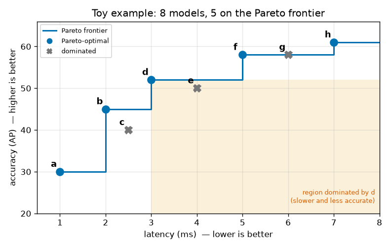
There are three things to read from Figure 12-1.
- The frontier is a staircase. The conceptual diagram in chapter 1 joined the points with slanted lines, but strictly speaking the frontier is a staircase plotting "the highest accuracy achievable with budget \(t\)". Even if the budget grows from 3.0 ms to 4.9 ms, the best usable model is still d.
- e lies inside the orange region. The region a point dominates is the quadrant to its lower right. The Pareto frontier consists of "the points that do not fall in the lower-right quadrant of any other point".
- g sits on the frontier line but is not on the frontier. It has the same accuracy as f and is slower.
Note · There is more than one choice of horizontal axis. The Pareto frontier changes depending on what is used as the "cost". Latency depends on the hardware and how it is measured, while compute (FLOPs) or parameter count is hardware-independent but can diverge from actual speed. The paper also notes that "configurations with similar parameter counts can have very different latencies". This chapter's experiment switches between three horizontal axes to see how the frontier changes.
The weight-sharing NAS framework
One set of weights, many configurations
Let us fix the notation. Call all of the model's weights \(\theta\), one configuration \(c\), and the search space \(\mathcal{C}\). In RF-DETR, a configuration is the values of the five knobs. For example, the paper's Nano is \(c = (\text{resolution } 384,\ \text{patch } 16,\ \text{windows } 2,\ \text{decoder } 2\text{ layers},\ \text{queries } 300)\).
Ordinary training fixes one configuration and reduces that configuration's loss. That is what chapter 11 did. If three sizes are needed, three sets of weights \(\theta_1, \theta_2, \theta_3\) are trained separately. Weight-sharing NAS trains a single set of weights \(\theta\) to work well in every configuration in the search space. The overall flow has three stages.
Figure 12-2 in the original is a diagram showing the three stages of weight-sharing NAS from left to right. The expensive training happens only once, and the search needs nothing but forward passes.
- ① Training (once): sample one configuration \(c\) (resolution · patch · windows) → run a forward pass with that configuration to get the loss \(\mathcal{L}(\theta; c)\) → update the weights \(\theta\), shared by all configurations, once. This loop repeats every step (the arrow returning to the first box).
- ② Search (no retraining): keep the trained \(\theta\) fixed and measure validation AP and latency for every configuration \(c\). All five knobs are swept, and decoder layers and queries are changed only here. The paper evaluates 6,468 configurations; this chapter's experiment evaluates 408.
- ③ Selection: plot one point per configuration on a plane with latency on the horizontal axis and AP on the vertical axis (every point comes from the same weights \(\theta\)), and pick the point on the Pareto frontier that fits the budget.
The place to look in Figure 12-2 is the returning arrow in ①. The configuration changes every step, but the weights being updated are always the same \(\theta\). And ② involves no training. The paper states that "we do not evaluate the search space until the base model has been fully trained on the target dataset". The search is merely a measurement on fully trained weights.
The training objective and its one-step approximation
Written as an equation, "a \(\theta\) that works well in every configuration" is the \(\theta\) that minimizes the average of the per-configuration losses. The paper does not write this equation and only describes the procedure ("at each training iteration, we uniformly sample a random model configuration and perform one gradient update"). Let us translate into equations what that procedure is solving.
- Why sampling one configuration per step reduces the average loss
- \(J(\theta) = \mathbb{E}_{c \sim \mathcal{C}}\big[\, \mathcal{L}(\theta; c) \,\big] = \frac{1}{|\mathcal{C}|} \sum_{c \in \mathcal{C}} \mathcal{L}(\theta; c)\)
- The objective \(J\) is the average loss over all configurations in the search space. \(c \sim \mathcal{C}\) means "sample from \(\mathcal{C}\) with every configuration having the same probability \(1/|\mathcal{C}|\)". Because the probabilities are equal, the expectation is just the arithmetic mean. (Equation (1) of the OFA paper likewise minimizes the sum of losses over all architectures with respect to the weights.)
- The derivative of a sum is the sum of the derivatives. Computing the exact gradient would require a forward and backward pass with every configuration at each step. With thousands of configurations, one step would become thousands of times more expensive.
- So we sample just one configuration \(c'\) and use its gradient \(\hat{g}\). The hat means "estimate".
- The expectation of \(\hat{g}\) is the sum weighted by each configuration's sampling probability \(1/|\mathcal{C}|\), which equals the exact gradient on the second line. Each individual step may be off, but on average it points in the right direction. This is exactly the same logic as minibatch gradient descent using a few images instead of the whole dataset (chapter 4); here there is simply one more thing being sampled: a few images and one configuration.
Let us check with numbers. Consider a toy problem where the weights are a single number \(\theta\) and there are only two configurations. Let the loss of configuration 1 be \(\mathcal{L}_1 = (\theta - 1)^2\) and the loss of configuration 2 be \(\mathcal{L}_2 = (\theta - 3)^2\). Configuration 1 wants \(\theta = 1\) and configuration 2 wants \(\theta = 3\).
- Hand calculation: a toy problem with two configurations
- \(J(\theta) = \tfrac{1}{2}(\theta - 1)^2 + \tfrac{1}{2}(\theta - 3)^2\)
- The losses of the two configurations are averaged.
- The derivative of \((\theta - k)^2\) is \(2(\theta - k)\), which multiplied by the leading \(\tfrac{1}{2}\) gives \((\theta - k)\). At \(\theta = 0\) the exact gradient is \(-4\).
- Sampling just one configuration gives a gradient of \(-2\) or \(-6\). Neither is \(-4\), but averaged with equal probability they give \(-4\). The direction (negative → increase \(\theta\)) is right in both cases.
- The average loss is smallest midway between the values the two configurations want. There, each configuration's loss is 1. Trained separately, each could have reached 0. When weights are shared, configurations have to compromise with each other.
The last line is the price of weight sharing. The OFA paper describes this as sub-networks "interfering" with each other. A real neural network has tens of millions of weights, so there is far more room than in the toy problem to satisfy many configurations at once, but it is not free. How much each configuration's accuracy drops (or rises) because of sharing can only be learned by experiment, and the latter part of this chapter measures it directly.
The resemblance to dropout, and architecture augmentation
The paper compares this training to the ensemble training of dropout (Srivastava et al., 2014). Dropout randomly switches off some neurons at each step, which amounts to alternately training a huge number of "thinned networks" that share weights. Weight-sharing NAS randomly changes the configuration instead of neurons. What they have in common is that one training run trains thousands of sub-networks together.
The paper adds an observation here: this training also acts as regularization. The paper calls this architecture augmentation. Just as data augmentation flips and crops images to show "different inputs with the same content", architecture augmentation alternates among "different architectures looking at the same image". The weights can no longer rely on tricks that only work at a particular resolution or patch size.
The evidence is Table 5 of the paper. At the Medium size, simply training with weight-sharing NAS while keeping all other conditions the same raised COCO AP from 54.3 to 54.6. This happened even though the configuration (patch 14, resolution 560) was unchanged. The paper writes that "counterintuitively, performance of the base configuration improves even though patch size 14 is not even in the NAS search space".
Caution · This gain depends on the conditions. The +0.3 AP was reported with a DINOv2 pretrained backbone, Objects365 pretraining, and COCO. As the toy problem above shows, weight sharing can in principle be a loss. When regularization is needed (the model is large relative to the data and overfits), the gain may win out; otherwise, the loss may. Which one appears in this chapter's mini experiment is checked later.
Grid search after training
Once training is done, a list of values is chosen for each knob and every combination of those lists is evaluated one by one. This is grid search. With five knobs, it amounts to visiting every cell of a five-dimensional grid. The work per cell is just measuring AP on the validation set and measuring latency.
This contrasts with early NAS, which used sophisticated search methods such as reinforcement learning or evolutionary algorithms. When evaluating one candidate required training, you had to be frugal about "which candidates to look at". When evaluation needs only forward passes, looking at all of them is the simplest and most reliable option. The paper estimates that this search took about 10,000 GPU hours (200 T4 GPUs × 48 hours). That is not cheap, but since it is measurement rather than training, it can be split up and run in parallel freely.
Extracting the Pareto frontier from the (AP, latency) points obtained in the search gives the model family. The paper's N · S · M · L · XL · 2XL are points chosen on that frontier. When new hardware comes along, only the latency needs to be re-measured, and when a new budget comes along, another point on the frontier can be chosen. In neither case is training repeated.
How it differs from OFA
RF-DETR's method started from OFA, but its training procedure differs. OFA reports that training by randomly sampling all sub-networks from the start causes a large accuracy drop due to interference between sub-networks, and proposed an ordering called progressive shrinking. The largest network is trained fully first, and then fine-tuning proceeds while smaller sub-networks are progressively added to the sampling range in the order kernel size → depth → width.
| OFA (Cai et al., 2019) | RF-DETR | |
| Target | Convolutional neural networks, image classification | DETR with a ViT backbone, detection and segmentation (end-to-end) |
| Knobs | Depth, width, kernel size, resolution | Patch size, number of decoder layers, number of queries, resolution, number of windows |
| Training order | Train the large network first, then add smaller sub-networks stage by stage (progressive shrinking) | No stages; configurations are sampled uniformly from the start |
| Learning rate schedule | A different schedule for each stage | No scheduler |
| Search | Train accuracy and latency predictors on a subset of sub-networks, then search with those predictors | Grid search over all configurations on the validation set |
The paper explains why RF-DETR dropped the stages: a staged schedule carries strong assumptions about "when the model converges", and those assumptions may not hold across diverse datasets. This is the same concern as the "scheduler-free training" seen in chapter 11. The paper calls its models "a scheduler-free, NAS-based family of models".
The nature of the knobs also differs. OFA's width and kernel-size knobs use a slice of the weights, so it had to sort which channels to keep or learn transformation matrices that derive small kernels from large ones. As shown below, most of RF-DETR's knobs "leave the weights untouched and change only the shape of the input or the length of the forward pass". This difference likely helps explain why stage-free training works, but the paper does not test this separately.
The five knobs: why the weights can be reused as-is
Reusing the weights when the architecture changes is not a given. If the number of layers changes, the number of weights changes, and if the input size changes, the matrix shapes no longer match. The question to ask for each knob is the same: which part of the weights is tied to this knob's value, and how is that tie broken? The answers are collected in a table first and then examined one by one.
| Knob | What changes | Tied weights | How the tie is broken | When it changes |
| (a) Patch size | Number of tokens, number of pixels per patch | Patch embedding kernel (\(p \times p\)), position embeddings | Convert the kernel with PI-resize, interpolate the position embeddings | Training + inference |
| (b) Number of decoder layers | Decoder depth | None (later layers are simply not used) | Apply a loss to every layer | Inference only |
| (c) Number of queries | Number of queries the decoder handles, maximum number of predictions | Trailing rows of the query embeddings | Use only the top ones selected by score | Inference only |
| (d) Resolution | Number of tokens, image detail | Position embeddings | Store at the largest grid and interpolate | Training + inference |
| (e) Number of windows | Range of tokens that can see each other in a window block | None | Only change how tokens are grouped | Training + inference |
Knob one: patch size
ViT cuts an image into \(p \times p\) pixel patches and turns them into tokens (chapter 6). For an image with side \(H\) pixels, the token grid has side \(g = H/p\) and the number of tokens is \(N = g^2\).
\(N = \left( \frac{H}{p} \right)^2 \qquad \text{e.g., for } H = 96 \text{: } \ p = 8 \to 12^2 = 144, \quad p = 12 \to 8^2 = 64, \quad p = 16 \to 6^2 = 36\)
Doubling the patch size cuts the number of tokens to 1/4. Since the computation per block is proportional to the number of tokens (linear layers) or its square (attention), the model becomes much faster; in exchange, each token lumps together a wide area and loses detail. In the paper's words, "smaller patches yield higher accuracy at greater computational cost".
The problem is the patch embedding. The patch embedding is a convolution with a \(p \times p\) kernel, and the kernel size is the patch size. An \(8 \times 8\) kernel trained with patch 8 cannot be applied to a \(16 \times 16\) patch. As previewed in chapter 6, the transform of FlexiViT (Beyer et al., 2023) solves this. The paper writes that it "interpolates between patch sizes during training with a FlexiViT-style transform".
Why not just interpolate the kernel like an image?
The first idea that comes to mind is to treat the kernel as a small image and enlarge it with bilinear interpolation. But what the patch embedding computes is the dot product \(\langle x, w \rangle\), and interpolation does not preserve dot products. If both the patch and the kernel are doubled in size, the number of summed terms grows from \(p^2\) to \(4p^2\), so the value becomes roughly 4 times larger. In the FlexiViT paper's terms, \(\langle x, w \rangle \approx \tfrac{1}{4} \langle \text{resize}(x),\ \text{resize}(w) \rangle\). If token magnitudes differ by a factor of 4 from training, the later blocks receive inputs they have never seen.
You might think "then just divide by 4", but that only matches the magnitude, not the values. Let us state exactly what we want: the dot product of the resized patch with the new kernel must equal the dot product of the original patch with the original kernel, for any patch.
Resizing is a matrix multiplication
Bilinear resizing is a linear operation. Each output pixel is a weighted average of input pixels (bilinear interpolation from chapter 8), and those weights are determined only by position, independent of the input values. A linear operation can be written as a matrix multiplication. If a \(p \times p\) patch is flattened into a vector \(x\) of length \(p^2\), the result of resizing it to \(p' \times p'\) is \(Rx\), where \(R\) is a \(p'^2 \times p^2\) matrix.
Finding \(R\) is simple. Resizing a patch that is "1 in one cell and 0 everywhere else" gives one column of \(R\). Resize \(p^2\) such patches in turn and stand them up as columns, and you get all of \(R\). Let us work it out for the smallest one-dimensional example: stretching a "patch" of length 2 to length 4.
- Hand calculation: the matrix R that stretches length 2 to length 4
- \(u_i = (i + 0.5) \cdot \frac{2}{4} - 0.5, \qquad u_0 = -0.25, \quad u_1 = 0.25, \quad u_2 = 0.75, \quad u_3 = 1.25\)
- Find where the center of the \(i\)-th output cell lies on the input's scale (the coordinate convention of chapter 8: treat cell centers as lying at integer + 0.5, scale by the ratio \(2/4\), then subtract 0.5). The two input cells sit at positions 0 and 1.
- Plug \(t = 0.25\) and \(0.75\) into linear interpolation \((1 - t)\, x_0 + t\, x_1\). \(u_0 = -0.25\) and \(u_3 = 1.25\) fall outside the input, so the value of the nearest cell is used as-is.
- The coefficients of \(x_0\) in the four equations above go in the first column and those of \(x_1\) in the second. The first column \((1, 0.75, 0.25, 0)\) is the result of stretching patch \((1, 0)\), and the second column is the result of stretching patch \((0, 1)\).
Deriving PI-resize
Now write the condition as an equation. Call the new kernel \(\hat{w}\) (length \(p'^2\)); what we want is \(\langle Rx, \hat{w} \rangle = \langle x, w \rangle\) for every patch \(x\).
- Enlarging the patch: a new kernel that preserves the dot product exactly
- \(\langle Rx,\ \hat{w} \rangle = (Rx)^\top \hat{w} = x^\top R^\top \hat{w}\)
- Write the dot product as a matrix product and use the fact that the transpose of a product is the product of the transposes in reverse order, \((Rx)^\top = x^\top R^\top\).
- For \(x^\top(R^\top \hat{w} - w) = 0\) to hold for every \(x\), the vector in parentheses must be the zero vector (setting \(x\) to that vector itself forces its squared length to be 0). The condition has become a system of linear equations in \(\hat{w}\).
- When the patch is enlarged (\(p' \gt p\)), there are more unknowns than equations. There is not one solution but infinitely many. We have to choose one of them.
- Look for a solution of the form "some original-size kernel \(z\), resized". \(R^\top R\) is a \(p^2 \times p^2\) square matrix, and for an enlarging resize the columns of \(R\) are linearly independent, so it is invertible.
- \(R (R^\top R)^{-1}\) is exactly the pseudo-inverse \((R^\top)^{+}\) of \(R^\top\). Check: \(R^\top \hat{w} = R^\top R (R^\top R)^{-1} w = w\). This is equation (3) of the FlexiViT paper, and the transform is called PI-resize (pseudo-inverse resize).
Why this one among infinitely many solutions? A solution of the form \(\hat{w} = Rz\) is the shortest solution. Every other solution has the form \(\hat{w} + n\) where \(n\) satisfies \(R^\top n = 0\). But \(\hat{w}^\top n = (Rz)^\top n = z^\top (R^\top n) = 0\), so the two are orthogonal, and by the Pythagorean theorem \(\| \hat{w} + n \|^2 = \| \hat{w} \|^2 + \| n \|^2 \ge \| \hat{w} \|^2\). Since \(n\) is a component that "has no effect on resized patches but responds to other inputs", this is the solution that contains no unnecessary component at all.
Let us carry the one-dimensional example through to the end. The kernel is \(w = (1, 3)\) and the patch is \(x = (2, 4)\). The original dot product is \(2 \cdot 1 + 4 \cdot 3 = 14\).
- Hand calculation: PI-resizing a length-2 kernel to length 4
- \(R^\top R = \begin{pmatrix} 1 & 0.75 & 0.25 & 0 \\ 0 & 0.25 & 0.75 & 1 \end{pmatrix} \begin{pmatrix} 1 & 0 \\ 0.75 & 0.25 \\ 0.25 & 0.75 \\ 0 & 1 \end{pmatrix} = \begin{pmatrix} 1.625 & 0.375 \\ 0.375 & 1.625 \end{pmatrix}\)
- Top left: \(1^2 + 0.75^2 + 0.25^2 + 0^2 = 1 + 0.5625 + 0.0625 = 1.625\). Top right: \(1 \cdot 0 + 0.75 \cdot 0.25 + 0.25 \cdot 0.75 + 0 \cdot 1 = 0.1875 + 0.1875 = 0.375\). By symmetry, the rest are the same.
- This is the inverse formula for a 2×2 matrix. The determinant is \(2.640625 - 0.140625 = 2.5\).
- \(0.65 - 0.45 = 0.2\), \(-0.15 + 1.95 = 1.8\).
- \(0.15 + 0.45 = 0.6\), \(0.05 + 1.35 = 1.4\). The new kernel differs from \((1, 1.5, 2.5, 3)\), the original kernel \((1, 3)\) simply stretched. The values are smaller overall (by as much as the number of terms grew).
- Exactly equal to the original dot product of 14. For comparison, the simply stretched kernel \(Rw = (1, 1.5, 2.5, 3)\) gives \(2 + 3.75 + 8.75 + 12 = 26.5\), and even correcting by the length ratio \(2/4\) gives \(13.25\), which differs from 14.
Figure 12-3 in the original is a diagram of what PI-resize preserves. The top row is the dot product of the original patch \(x\) (\(p \times p\)) and kernel \(w\) (\(p \times p\)), i.e., the token \(\langle x, w \rangle\) seen during training. Moving down, the patch becomes \(Rx\) (\(p' \times p'\)) through the resize \(R\), and the kernel becomes \(\hat{w}\) (\(p' \times p'\)) through PI-resize \((R^\top)^{+}\). The token \(\langle Rx, \hat{w} \rangle\) in the bottom row equals \(\langle x, w \rangle\) in the top row (exactly, when enlarging). Because the kernel is changed so that the dot product of the enlarged patch with the new kernel equals that of the original patch with the original kernel, the tokens received by later blocks do not change.
This result can also be read another way. In actual use, a large patch \(x'\) (length \(p'^2\)) is not a stretched small patch but a genuine \(p' \times p'\) patch cut directly from the image. The value the new kernel produces then is
\(\langle x',\ \hat{w} \rangle = x'^\top R\,(R^\top R)^{-1} w = \big\langle (R^\top R)^{-1} R^\top x',\ w \big\rangle = \langle R^{+} x',\ w \rangle\)
Here \(R^{+} x' = (R^\top R)^{-1} R^\top x'\) is "the small patch that, when resized, comes closest to \(x'\)", i.e., the \(p \times p\) patch that best shrinks \(x'\) in the least-squares sense. So reading a large patch with a PI-resized kernel is the same as shrinking the large patch well to the original size and then reading it with the original kernel. What the kernel learned (which patterns it responds to) stays the same; only its field of view widens.
Note · When shrinking the patch
If \(p' \lt p\), then \(R^\top \hat{w} = w\) has more equations than unknowns and generally has no solution. That is natural, since a small kernel cannot hold all the fine patterns of a large kernel. In this case FlexiViT looks for the \(\hat{w}\) that is "least wrong on average". Assuming patches follow a standard normal distribution, the answer is the least-squares solution minimizing \(\| w - R^\top \hat{w} \|^2\), which is also given by the same formula \(\hat{w} = (R^\top)^{+} w\) (FlexiViT Appendix A.2). The pseudo-inverse is an operation that gives "the shortest solution when there are many, and the least-wrong solution when there are none". In practice, FlexiViT stores the kernel at a large size (32×32) and converts it to the size it needs.
Implementation and verification
It works the same way in two dimensions. Build \(R\) by resizing 64 basis patches of size \(8 \times 8\), compute the pseudo-inverse once, and multiply it into each channel of the kernel. Chapter 9's WindowedViT calls patch_resize_fn when the patch size changes, so this function can simply be plugged in.
code/ch12_nas.py · pi-resize
def resize_matrix(old: int, new: int, ndim: int = 2) -> torch.Tensor:
    """쌍선형 리사이즈를 행렬로 쓴 것. 돌려주는 값 R: (new^ndim, old^ndim), float64.

    리사이즈는 선형 연산이다: 리사이즈(a·x + b·y) = a·리사이즈(x) + b·리사이즈(y). 그러므로 "한 칸만 1 이고 나머지는 0" 인
    패치(기저 벡터)들을 리사이즈한 결과를 열로 세우면 그것이 곧 행렬 R 이고, 어떤 패치 x 든 리사이즈(x) = R·vec(x) 다.
    ndim=1 은 본문의 1차원 손계산 예를 위한 것.
    """
    basis = torch.eye(old**ndim, dtype=torch.float64).reshape(old**ndim, 1, *([old] * ndim))  # 기저 패치 old^ndim 장
    mode = "bilinear" if ndim == 2 else "linear"
    resized = F.interpolate(basis, size=[new] * ndim, mode=mode, align_corners=False)  # (old^ndim, 1, new, …)
    return resized.reshape(old**ndim, new**ndim).T  # j 번째 열 = j 번째 기저 패치를 리사이즈한 것

_PI_CACHE: dict = {}

def pi_resize_matrix(old: int, new: int, ndim: int = 2) -> torch.Tensor:
    """PI-resize 행렬 P = (Rᵀ)⁺: (new^ndim, old^ndim).  새 커널 = P · vec(원래 커널).

    키울 때(new ≥ old)는 P = R (RᵀR)⁻¹ 이고 Rᵀ P = I — 리사이즈한 패치와 새 커널의 내적이 원래 내적과 정확히 같다.
    줄일 때(new < old)는 정확한 답이 없고, P 는 ‖w − Rᵀ ŵ‖² 을 가장 작게 하는 ŵ 를 준다.
    """
    key = (old, new, ndim)
    if key not in _PI_CACHE:
        _PI_CACHE[key] = torch.linalg.pinv(resize_matrix(old, new, ndim).T)
    return _PI_CACHE[key]

def pi_resize_patch_embed(weight: torch.Tensor, new_patch: int) -> torch.Tensor:
    """FlexiViT 의 PI-resize 로 패치 임베딩 합성곱의 가중치를 다른 패치 크기로 바꾼다.

    weight: (C, 3, p, p) → (C, 3, p', p').  출력 채널 · 입력 채널마다 따로 같은 행렬 P 를 곱한다.
    WindowedViT.patch_resize_fn 에 끼워 쓴다 (순전파마다 불린다. P 는 한 번만 계산해 둔다. 기울기는 P 를 거슬러 흐른다).
    """
    old_patch = weight.shape[-1]
    if new_patch == old_patch:
        return weight
    P = pi_resize_matrix(old_patch, new_patch).to(weight)  # (p'², p²)
    flat = weight.reshape(-1, old_patch * old_patch)  # (C·3, p²): 커널의 채널마다 한 줄
    return (flat @ P.T).reshape(*weight.shape[:2], new_patch, new_patch)
Below are the values from running the hand-calculation example in code, along with the dot-product preservation error measured on real patches. The kernel is the patch embedding of the mini RF-DETR trained in chapter 11 (96 channels × RGB × 8 × 8), and the patches are 2,000 random \(8 \times 8\) crops from validation images. Three methods are compared: PI-resize, chapter 9's simple version (bicubic interpolation followed by multiplying by \((p/p')^2\)), and bilinear interpolation alone.
[PI-resize] 1차원 손계산 예: 길이 2 인 패치를 길이 4 로
  R = [[1.0, 0.0], [0.75, 0.25], [0.25, 0.75], [0.0, 1.0]]
  RᵀR = [[1.625, 0.375], [0.375, 1.625]]  (RᵀR)⁻¹ = [[0.65, -0.15], [-0.15, 0.65]]
  w = [1, 3], x = [2, 4]:  ⟨x, w⟩ = 14.0
  Rx = [2.0, 2.5, 3.5, 4.0]  ŵ = P w = [0.2, 0.6, 1.4, 1.8]  ⟨Rx, ŵ⟩ = 14.0
  단순 보간 Rw = [1.0, 1.5, 2.5, 3.0]  ⟨Rx, Rw⟩ = 26.5  길이 비로 보정 (2/4)·⟨Rx, Rw⟩ = 13.25
  check Rᵀ ŵ = w 인가: [1.0, 3.0] | P = R(RᵀR)⁻¹ 과의 차이 1.1e-16
  check 2차원 R (8→12, 모양 (144, 64)) 과 F.interpolate 의 차이: 1.1e-16
[PI-resize] 내적 보존: 11장 모델의 패치 임베딩 (96, 3, 8, 8), 검증 그림에서 자른 8×8 패치 2000개
  새 패치 | 방법                        | 상대 오차 ‖⟨Rx, ŵ⟩ − ⟨x, w⟩‖ / ‖⟨x, w⟩‖ | 토큰 크기의 비 ‖⟨Rx, ŵ⟩‖ / ‖⟨x, w⟩‖
        4 | PI-resize                   |     1.57e-01                             | 0.9853
        4 | bicubic x (p/p')^2 (ch09)   |     1.98e-01                             | 1.0134
        4 | bilinear only               |     7.58e-01                             | 0.2463
        6 | PI-resize                   |     9.99e-02                             | 0.9947
        6 | bicubic x (p/p')^2 (ch09)   |     1.17e-01                             | 0.9958
        6 | bilinear only               |     4.71e-01                             | 0.5511
       10 | PI-resize                   |     1.54e-15                             | 1.0000
       10 | bicubic x (p/p')^2 (ch09)   |     7.22e-02                             | 0.9884
       10 | bilinear only               |     5.47e-01                             | 1.5325
       12 | PI-resize                   |     1.87e-15                             | 1.0000
       12 | bicubic x (p/p')^2 (ch09)   |     7.16e-02                             | 0.9870
       12 | bilinear only               |     1.22e+00                             | 2.2180
       16 | PI-resize                   |     1.68e-15                             | 1.0000
       16 | bicubic x (p/p')^2 (ch09)   |     7.41e-02                             | 0.9871
       16 | bilinear only               |     2.95e+00                             | 3.9402
       24 | PI-resize                   |     1.23e-15                             | 1.0000
       24 | bicubic x (p/p')^2 (ch09)   |     6.40e-02                             | 0.9885
       24 | bilinear only               |     7.89e+00                             | 8.8867
       32 | PI-resize                   |     1.15e-15                             | 1.0000
       32 | bicubic x (p/p')^2 (ch09)   |     6.96e-02                             | 0.9877
       32 | bilinear only               |     1.48e+01                             | 15.7752
- Figure 12-4: ch12-pi-resize.png Left: one kernel (red channel) and its enlargement to \(16 \times 16\) by the three methods (same color scale). Middle: token values before (horizontal) and after (vertical) enlarging both patch and kernel from 8 → 16. The black line is "unchanged". Right: relative token error by new patch size (log axis). Left of the vertical dotted line is the shrinking case.
- (Figure content) Left: one patch embedding kernel and its enlargement to 16×16 by the three methods. Middle: scatter plot of token values before and after resizing. Right: dot-product preservation error by new patch size.
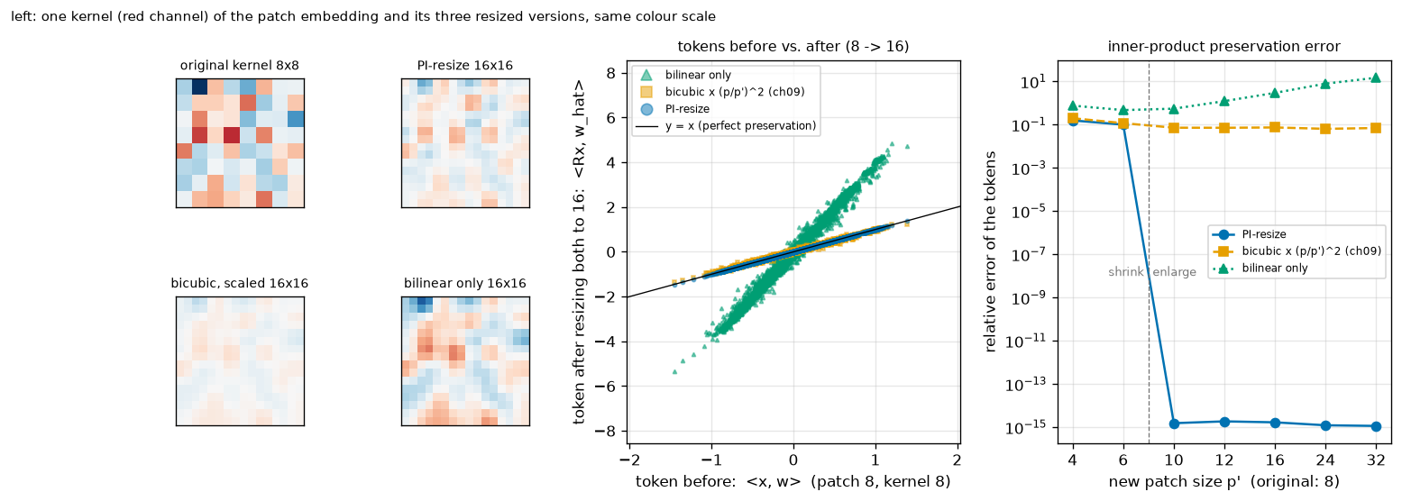
What to read from the output and Figure 12-4:
- When enlarging, the PI-resize error is on the order of \(10^{-15}\). That is merely 64-bit floating-point rounding error; the values are exactly equal, as derived. In the middle panel, the blue dots lie right on the black line.
- Bilinear interpolation alone inflates the tokens. For 8 → 16 the magnitude ratio is 3.94, just the "about 4 times" estimated earlier (8 → 32 gives 15.8, about 16 times). In the middle panel the green dots form a line 4 times steeper than the black line. In the left panel, too, the bilinear version has about the same color intensity as the original kernel, but with 4 times as many cells its sum is about 4 times larger.
- Chapter 9's simple version matches the magnitude but is off by about 7% in value. Multiplying by \((p/p')^2\) brings the magnitude ratio to 0.99, but a relative error of 0.07 remains. This is the same kind of discrepancy as 13.25 versus 14 in the hand calculation.
- When shrinking, even PI-resize is not exact. The error is 0.10 for 8 → 6 and 0.16 for 8 → 4. Information is lost, so no method can be exact; among them, PI-resize has the smallest error.
- In the left panel, the PI-resize and simple-version kernels are faint. With 4 times as many cells, each cell's value got smaller. The PI-resize kernel shows a fine pattern absent from the simple version; this is the component added to match the dot product exactly.
If the tokens are the same, is the model's output also the same? Figure 4 of the FlexiViT paper enlarges both images and patches by the same factor on a trained ViT and measures accuracy, reporting that only PI-resize preserved accuracy when enlarging. We ran the same experiment with chapter 11's mini RF-DETR. This model was trained only at resolution 96 · patch 8 and has never seen another patch size. Enlarging the image and patch together keeps the token grid at 12×12.
[PI-resize] 11장 모델(해상도 96 · 패치 8 로만 학습)에서 그림과 패치를 같은 배율로 키운다. 원래 AP 0.9345
  해상도 / 패치 (격자) | PI-resize                   | bicubic x (p/p')^2 (ch09)   | bilinear only
   120 / 10 (12×12)     | AP 0.9348                   | AP 0.9347                   | AP 0.8585
   144 / 12 (12×12)     | AP 0.9352                   | AP 0.9344                   | AP 0.7579
   192 / 16 (12×12)     | AP 0.9351                   | AP 0.9348                   | AP 0.6315
- With PI-resize, AP stays the same (0.9345 → 0.9348 – 0.9352). This holds at patch sizes 10 · 12 · 16, never seen before, without retraining. (Resizing the whole image and resizing each patch differ slightly at patch borders, so the tokens are not perfectly identical. The difference is within 0.001 in AP.)
- Bilinear interpolation alone collapses (0.8585 → 0.7579 → 0.6315). It gets worse as the scale factor grows, that is, as the tokens get larger than during training. This fits the explanation that the cause is the "drastic change in token norm" FlexiViT describes.
- Chapter 9's simple version also preserves AP (0.9344 – 0.9348). In this experiment the 7% token error did not affect AP. The difference between the exact and approximate transforms did not show up with this small model and easy data; matching the magnitude was what mattered. This tutorial uses PI-resize, whose derivation is clear.
Note · The paper and the public code. The RF-DETR paper says only "a FlexiViT-style transform" and does not give the specific formula. The public code examined by this tutorial (the rfdetr package) fixes the patch size when the model is built and did not include NAS training code that changes the patch size on every forward pass. The pi_resize_patch_embed built here is a direct implementation of the FlexiViT paper's formula; whether it matches RF-DETR's internal implementation could not be confirmed.
When the patch size changes, the token grid changes too, so the position embeddings must be adjusted as well. This is the same problem as the resolution knob, so it is covered there.
Knob two: number of decoder layers
The decoder is a stack of identically shaped layers, each of which refines the query embeddings a little. Recall the auxiliary losses from chapter 7. The DETR family does not apply the loss only to the last layer's output; it attaches the same head to every layer's output and applies the same loss. Chapter 11's total loss did exactly that.
\(\mathcal{L}(\theta; c) = \sum_{l=0}^{L} \mathcal{L}_{\text{det}}\big( \hat{y}^{(l)},\ y \big)\)
\(\hat{y}^{(l)}\) is the prediction made by attaching the head to queries that have passed through only up to decoder layer \(l\), \(y\) is the ground truth, and \(\mathcal{L}_{\text{det}}\) is the classification + box loss after matching. \(l = 0\) is the encoder proposal before entering the decoder (two-stage query selection from chapter 10). The mini model has \(L = 3\), so four sets of losses were summed.
Auxiliary losses were originally a device to help train deep decoders. But reading this equation again reveals another meaning: the model was trained so that \(\hat{y}^{(l)}\) is a good prediction on its own for every \(l\). Then at inference you can stop at layer \(l\) and use its output as the answer. A model stopped at layer \(l\) was never trained separately, but it is an "already trained sub-network" that received a loss throughout training.
So this knob has no tie to break. The forward pass simply ends early. This is why, in chapter 10's check, the difference between "the output using only \(k\) decoder layers" and "the \(k\)-th auxiliary output of the full model" was exactly 0. The paper notes that this idea was already used in RT-DETR and others (since each layer is supervised independently, layers can be cut off at inference), and goes further.
- 0 layers: remove the decoder entirely. Only the encoder proposals remain. With no self-attention among queries and no cross-attention reading the feature map, it becomes much faster. The paper writes that this model resembles "an NMS-free, YOLO-style single-stage detector", because all it does is output a score and box for each cell of the feature map and pick the top few.
- Remove just the last layer. The paper (Appendix B) reports a 10% reduction in latency and a 2-point drop in mAP.
- The effect is larger for segmentation. RF-DETR-Seg produces masks at every decoder layer (chapter 13), so reducing the decoder also reduces the segmentation computation.
In chapter 11's mini experiment, the AP with 0 · 1 · 2 · 3 decoder layers was 0.8928 · 0.9289 · 0.9332 · 0.9347. The first layer provides most of the gain, and the gains shrink with later layers. These numbers come up again in this chapter's search.
Knob three: number of queries
The number of queries is the maximum number of predictions the model can make and also the decoder's workload. The decoder's self-attention does computation proportional to the square of the number of queries, while cross-attention and the FFN do computation proportional to the number of queries. RF-DETR trains with 300 queries. But for data with a few dozen objects per image at most, most of the 300 are computed only to output "no object".
To reduce the queries, you must decide which queries to drop. If the queries were learned vectors unrelated to the image, as in chapter 7's DETR, there would be no way to know in advance which ones matter less. RF-DETR uses two-stage query selection (chapter 8, chapter 10), so things are different. The queries start from the top \(N\) cells, ranked by class score, among all cells of the feature map. They are already ranked.
- Reducing queries = cutting the ranking from the top
- \(s_j = \max_k\ \sigma(z_{jk}), \qquad j = 1, \dots, HW\)
- For each cell \(j\) of the feature map, the largest sigmoid of the class logits \(z_{jk}\) from the encoder-side classification head is taken as that cell's score \(s_j\). In the paper's words, "the maximum of the sigmoid of the per-token class logits from the encoder output". (Since the sigmoid preserves order, ranking by the maximum logit gives the same result.)
- Select \(N\) cells in decreasing order of score. During training \(N = 300\) (12 for the mini model).
topkreturns results in descending order of score.
- Selecting only \(N'\) is the same as selecting \(N\) and keeping just the first \(N'\). In other words, "drop queries starting from the lowest score". The query embeddings (
query_feat,refpoint_embed) likewise use only the first \(N'\) rows, following the ranking.
What gets dropped are the cells the encoder considers least likely to be objects. If an image has 5 objects, they will be in the top few rows of the ranking, and cutting off ranks 200 to 300 loses almost nothing. Appendix B of the paper (Figure 4) reports that dropping the 100 lowest-scoring queries in Nano barely reduces performance while slightly improving latency.
There are two caveats.
- The outputs of the remaining queries change slightly too. In the decoder's self-attention, queries look at each other. With fewer counterparts, the results differ (in chapter 10's check, reducing 12 queries to 6 with untrained weights changed the remaining queries' logits by up to 0.298). Unlike removing decoder layers, this is not "a subset of exactly the same output".
- It is a situation never seen during training. The number of queries is not changed during training. Whether the model works well with fewer queries has to be checked by experiment, and the paper and this chapter's experiment measure it.
The paper interprets this knob as follows: the Pareto-optimal number of queries implicitly encodes dataset statistics (how many objects an image has on average). In fact, the low-latency models found on RF100-VL used fewer queries than COCO models at the same latency, and the paper attributes this to RF100-VL having fewer objects per image than COCO (Appendix L).
Note · This differs from num_select in chapter 14. The num_select adjusted in chapter 14 is the number of predictions kept by post-processing. The decoder still computes all 300 queries, so the network's computation does not decrease. This chapter's query knob reduces the queries fed into the decoder themselves.
Knob four: input resolution
Raising the resolution shows small objects with more pixels; lowering it reduces the tokens and speeds things up. This knob moves the same equation \(N = (H/p)^2\) as patch size, in the opposite direction. The ViT block weights do not depend on the number of tokens (attention uses the same matrices no matter how many tokens there are; chapter 5). As seen in chapter 6, only two sets of weights are tied to image size.
- Patch embedding: independent of resolution (tied only to patch size).
- Position embeddings: there is one vector per cell of the token grid, so they are tied to the grid size \(g \times g\).
The position embeddings are handled with the method from chapter 6: reshape back into a 2D grid and interpolate to the required size. The paper's approach is to store them at the largest grid: "we keep \(N\) position embeddings corresponding to the largest resolution divided by the smallest patch size, and interpolate them for smaller resolutions or larger patches." With the paper's training grid (resolution up to 960, patch as small as 8), that is \(960 / 8 = 120\) cells per side. This chapter's mini experiment uses \(128 / 8 = 16\) cells. Storing a large grid and shrinking it always goes in the direction of "reducing information that exists", so less is lost than stretching a small grid.
What about after the backbone? The projector is convolutional, so it works regardless of the feature map size. Two-stage query selection applies the same head to every cell, so any number of cells works. Deformable attention reads the feature map with normalized coordinates, so the formula is the same even if the map size changes (chapter 8). And the values output by the box head are also normalized coordinates. The decision in chapter 2 to express boxes as ratios of the image size pays off here. Whether the image is shrunk to 64 or enlarged to 128, the ground-truth box \((c_x, c_y, w, h)\) does not change by a single digit, and the head does not need to know the resolution.
Resolution also varied in LW-DETR. Back then, however, it was data augmentation (multi-scale training) to help training, and inference used a single fixed resolution. RF-DETR promoted the same thing to a knob. In the words of the paper's Appendix A, "we include resolution as a tunable knob in the NAS search space, whereas LW-DETR uses it as a form of data augmentation." The training-time handling also differs slightly. LW-DETR changed the size per image and padded the rest to match the largest image in the batch, whereas RF-DETR changes the size per batch. No computation is wasted on padded regions, and every position embedding resolution appears evenly during training.
Knob five: number of windows
The windowed attention from chapter 9 divides the token grid into \(W \times W\) windows, and in window blocks attention happens only among tokens in the same window (\(W\) is the number of windows per side). In global blocks, all tokens see each other. As confirmed in chapter 9, windowed attention has no dedicated weights. All it does is rearrange tokens by window and move them to the batch axis; the attention itself is computed by the same weights of the same block. So changing the number of windows has no tie to break. Only the grouping changes.
Let us count pairs to see what is gained and lost by adding windows. On the mini model's default grid (\(g = 12\), \(N = 144\)) there are 4 window blocks and 2 global blocks. Because the DINOv2 backbone needs a CLS token, RF-DETR duplicates one CLS token per window. The number of tokens per window is \(N/W^2 + 1\).
- Hand calculation: number of attention pairs by number of windows (12×12 grid)
- \(\text{one window block: } \ W^2 \left( \frac{N}{W^2} + 1 \right)^2, \qquad \text{one global block: } \ \left( N + W^2 \right)^2\)
- In a window block, each of the \(W^2\) windows forms pairs among its own tokens. In a global block, all \(N\) patch tokens and the \(W^2\) CLS tokens form one sequence and see each other.
- With one window, window blocks and global blocks are the same. The total over six blocks is \(6 \times 21{,}025 = 126{,}150\) pairs.
- \(36 + 1 = 37\) tokens per window. The total is \(4 \times 5{,}476 + 2 \times 21{,}904 = 21{,}904 + 43{,}808 = 65{,}712\) pairs, 52% of \(W = 1\).
- \(9 + 1 = 10\) tokens per window. Window blocks got cheaper, but global blocks actually got more expensive as the CLS tokens grew to 16. The total is 88% of \(W = 2\), a small gain compared with the halving from 1 → 2.
As windows increase, the gain shrinks quickly while the cost of duplicated CLS tokens grows. On the accuracy side, distant tokens can no longer exchange information in window blocks. The observation in the paper's Appendix L matches this: most Pareto-optimal RF-DETR models used 2 windows (for LW-DETR, 4 was optimal). The paper explains the difference by the CLS token. LW-DETR's CAEv2 backbone has no CLS token, whereas DINOv2 uses the CLS token as central to its pretraining, and since CLS must be duplicated per window, more windows means lower runtime efficiency. In global blocks, the per-window CLS tokens see each other too, and the other tokens see all CLS tokens.
What changes during training versus only at inference
The five knobs fall into two groups. The paper's Appendix A states clearly that "decoder layers and queries are reduced only at inference".
- Changed from training onward: resolution, patch size, number of windows. These three change the shape of the input to the backbone. The weights need to experience inputs of various shapes, so they are changed randomly at every step.
- Changed only at inference: number of decoder layers, number of queries. Training always uses the largest setting (6 layers, 300 queries). Layers can be reduced at inference thanks to the auxiliary losses, and queries thanks to the score ranking.
The grid in the paper's Appendix A is as follows.
| Knob | Values sampled during training | Values swept during search (inference) |
| Resolution | 320, 384, 448, 512, 576, 640, 704, 768, 832, 896, 960 (11 values, steps of 64) | |
| Patch size | 8, 10, 12, 16, 20, 24, 32 (7 values) | 8, 10, 12, 14, 16, 20, 24, 32 (8 values) |
| Number of decoder layers | 6 | 0, 1, 2, 3, 4, 5, 6 (7 values) |
| Number of windows | 1, 2, 4 | |
| Number of queries | 300 | 50, 100, 200, 300 (4 values) |
The paper states that the search evaluated 6,468 configurations and breaks the number down as: 11 resolutions × 7 patch sizes × 7 decoder layer counts × 3 window counts × 4 query counts.
- Counting the configurations
- \(11 \times 7 = 77, \qquad 77 \times 7 = 539, \qquad 539 \times 3 = 1{,}617, \qquad 1{,}617 \times 4 = 6{,}468\)
- If the knobs are independent, the number of combinations is the product of the number of values for each knob. This matches the paper's figure.
- However, the inference grid in the same appendix lists 8 patch sizes, including 14. Counting 8 gives 7,392. The paper's 6,468 counts 7 patch sizes, and the paper does not explain the discrepancy. Here we reproduce the paper's notation as-is and record both facts.
- During training, decoder layers and queries are fixed, so what is sampled is a combination of (resolution, patch, windows). The 6,468 at search time is this multiplied by 7 decoder layer counts and 4 query counts (\(231 \times 28 = 6{,}468\)).
Patch size 14 is an interesting value. DINOv2 was pretrained with patch size 14 (chapter 6), yet 14 is not in the training grid. The description of Table 5 also says "patch size 14 is not in the NAS search space". That the performance of that configuration still improved with NAS training was the evidence for architecture augmentation seen earlier.
Also, this count is a plain product that ignores divisibility. For example, resolution 320 is not divisible by patch 12. The paper does not say how it handled such combinations (for instance, whether the resolution was rounded to a nearby multiple). This chapter's mini experiment excludes non-divisible combinations from the search space.
The paper mentions two costs.
- Training time: about 2 – 4 times the non-NAS baseline (depending on the dataset). In exchange, every size comes out of that one training run. Without NAS, each size would have to be retrained.
- Search time: estimated at about 10,000 GPU hours (200 T4 GPUs × 48 hours = 9,600 GPU hours).
Reading the architectures the paper found
Configurations on the Pareto frontier
The Pareto-optimal configurations found on COCO are in Table 7 (detection) and Table 8 (segmentation) of the paper. The last column, "grid", is the resolution divided by the patch size, computed and added by this tutorial.
| Detection (Table 7) | Resolution | Patch | Windows | Decoder layers | Queries | Backbone | Grid (resolution ÷ patch) |
| N | 384 | 16 | 2 | 2 | 300 | DINOv2-S | 24 |
| S | 512 | 16 | 2 | 3 | 300 | DINOv2-S | 32 |
| M | 576 | 16 | 2 | 4 | 300 | DINOv2-S | 36 |
| L | 704 | 16 | 2 | 4 | 300 | DINOv2-S | 44 |
| XL | 700 | 20 | 1 | 5 | 300 | DINOv2-B | 35 |
| 2XL | 880 | 20 | 2 | 5 | 300 | DINOv2-B | 44 |
| Max | 828 | 12 | 1 | 6 | 300 | DINOv2-B | 69 |
| Segmentation (Table 8) | Resolution | Patch | Windows | Decoder layers | Queries | Backbone | Grid (resolution ÷ patch) |
| N | 312 | 12 | 1 | 4 | 100 | DINOv2-S | 26 |
| S | 384 | 12 | 2 | 4 | 100 | DINOv2-S | 32 |
| M | 432 | 12 | 2 | 5 | 200 | DINOv2-S | 36 |
| L | 504 | 12 | 2 | 5 | 300 | DINOv2-S | 42 |
| XL | 624 | 12 | 2 | 6 | 300 | DINOv2-S | 52 |
| 2XL | 768 | 12 | 2 | 6 | 300 | DINOv2-S | 64 |
| Max | 890 | 10 | 1 | 6 | 300 | DINOv2-S | 89 |
Here is what the tables show, together with the observations in the paper's Appendix L.
- Every knob is used. All five knobs take different values across the Pareto-optimal family. The paper writes that this means the search space was chosen usefully, and suggests that widening the search space might bring further gains.
- Patch size is constant within a family. It is 16 for detection models with a DINOv2-S backbone, 20 with a DINOv2-B backbone, and 12 for segmentation models.
- Within a family, size grows mainly through resolution. From detection N → L, resolution grows from 384 → 704 (grid 24 → 44) and the decoder grows from 2 → 4 layers. Encoder-side computation (patch · windows · resolution) and decoder-side computation (layers · queries) grow together.
- Windows are mostly 2. This fits the cost of CLS token duplication discussed in the previous section.
- Detection keeps queries at 300 and increases decoder depth, while segmentation moves both together. Segmentation N · S use 100 queries with 4 decoder layers. The paper interprets this as the segmentation head needing a reasonably deep decoder to do its job, with the latency offset by reducing the number of queries ("a thin, deep decoder", versus "a wide, shallow decoder" for detection).
- XL's resolution of 700 and Max's 828 · 890 are not in the Appendix A grid (steps of 64). So the configurations in Tables 7 · 8 did not come solely from that grid, but the paper does not explain separately how these values were chosen.
The number of spatial locations drives performance
The most useful observation in Appendix L is this: RF-DETR's performance correlates more strongly with the ratio of resolution to patch size, that is, the number of spatial locations (tokens per side \(g = H/p\)), than with either one alone. The paper's explanation is exactly what we saw in chapter 6. After the image is cut into patches and projected, the ViT does not know how many pixels the original image had. All the blocks see is \(g \times g\) tokens.
To check this, the paper built a separate model family with the resolution fixed at 640 and only the patch size varied: patch 27 for Nano, 21 for Small, and 18 for Medium. Computing the grids gives \(640/27 \approx 23.7\), \(640/21 \approx 30.5\), and \(640/18 \approx 35.6\), close to the 24 · 32 · 36 of the original family (the paper does not say how non-integer values were handled). The results were reportedly "nearly identical" to the original Pareto-optimal family. Moreover, patches 27 and 18 were never seen during training.
This observation did not hold for segmentation, because segmentation features are always produced at 1/4 of the input resolution (chapter 13). Raising the resolution increases both the number of spatial locations and the mask detail, but enlarging only the patch changes the resolution of the mask features even if the number of spatial locations stays the same. The two knobs no longer collapse into a single effect.
A table turning one knob at a time
Table 5 of the paper shows the path from LW-DETR (M) to RF-DETR (M) one row at a time. Here are only the later, NAS-related rows (COCO, T4 latency).
| Step | GFLOPs | Latency (ms) | AP | Interpretation |
| (Before NAS) + additional Objects365 pretraining | 78.2 | 4.7 | 54.3 | Starting point. Patch 14, resolution 560 |
| + Train with weight-sharing NAS | 78.2 | 4.7 | 54.6 | Same configuration, yet +0.3 (architecture augmentation) |
| Patch 14 → 16, resolution 560 → 640 | 78.5 | 4.7 | 54.4 | Grid 40 → 40. Nearly unchanged |
| Resolution 640 → 576 | 64.2 | 4.0 | 53.6 | Grid 40 → 36. Faster, −0.8 |
| Windows 4 → 2 | 63.7 | 4.3 | 54.3 | +0.7, latency +0.3 ms |
| Decoder 3 → 4 layers | 64.8 | 4.4 | 54.6 | +0.3, latency +0.1 ms |
| Queries 300 → 300 | 64.8 | 4.4 | 54.6 | No change. Same configuration as M in Table 7 |
This table shows well how the knobs are used. Lowering the resolution buys 0.7 ms (−0.8 AP), and part of that headroom is spent again on windows and decoder layers to win back AP (+1.0 AP, +0.4 ms). The net result is the same AP of 54.6, 0.3 ms faster (4.7 → 4.4 ms) than the starting point. That is a spot no single knob could reach on its own. The third row is also worth noting. Changing the patch and resolution together to keep the grid at 40 leaves AP and latency nearly unchanged. This is the same story as the observation about the number of spatial locations.
Unseen configurations and fine-tuning
Configurations not seen during training (Appendix F). Figure 5 of the paper plots performance while varying resolution and patch size one at a time, with values seen and not seen during training drawn with different markers. The unseen configurations follow the trend line formed by the seen ones. The paper cites this as evidence that "RF-DETR generalizes beyond the configurations encountered during training". Patches 27 · 18 in the previous section are the same kind of evidence. It means the search space behaves not as a sparse grid but as a continuum that smoothly fills in the gaps, which matters in practice.
Fine-tuning after NAS (Appendix G). Once you pick one configuration on the Pareto frontier, wouldn't training a bit more with that configuration fixed make it better? It seems plausible, since the weights no longer need to compromise with other configurations. The paper's answer is that "on COCO there is almost no gain". The AP changes in Table 15 are as follows.
| Size | N | S | M | L | XL | 2XL |
| NAS as-is (COCO AP) | 48.0 | 52.9 | 54.7 | 56.5 | 58.6 | 60.1 |
| Change after fine-tuning | +0.4 | +0.1 | +0.0 | +0.0 | +0.3 | +0.1 |
The paper's interpretation is this: architecture augmentation acted as strong regularization, and removing that regularization during fine-tuning tilts the model toward overfitting, so the gain disappears. The paper notes that OFA reported a similar observation. On RF100-VL, by contrast, fine-tuning helped a little (Table 4: N 57.8 → 58.6, S 60.9 → 61.2, M 61.7 → 62.0, 2XL 63.3 → 63.5). The paper speculates that on small datasets the regularization of architecture augmentation takes more than 100 epochs to converge. The paper's position is therefore that fine-tuning is "optional and usually unnecessary in real deployments".
A different answer for each dataset
Dataset characteristics and knobs (Appendix H). The paper found the optimal Medium-size configuration for each of the 100 datasets in RF100-VL and fit straight lines between dataset characteristics and knob values (Table 17). Two stand out by coefficient of determination \(R^2\): number of spatial locations versus number of windows (\(R^2 = 0.492\)), and average object size versus number of spatial locations (\(R^2 = 0.148\), negative slope: the smaller the objects, the more spatial locations are needed). The rest are weak. For example, objects per image versus number of queries has \(R^2 = 0.019\), and number of classes versus number of decoder layers has \(R^2 = 0.026\). The body text of the appendix says some of these pairs show a "strong correlation", but the caption of Figure 6 in the same appendix concludes that "dataset characteristics have only a modest influence on architecture choice … with no clear deterministic relationship". The latter is the one consistent with the numbers in the table. The conclusion to take from this appendix is that it is hard to predict the optimal configuration in advance from a few dataset statistics, which is why search is needed.
Using the architecture found on COCO as-is (Appendix I). Then can the configurations found on COCO (Table 7) simply be carried over to other data? Table 18 compares the two on RF100-VL (AP).
| Size | N | S | M | L | XL | 2XL |
| COCO configuration as-is (fixed architecture) | 57.7 | 60.2 | 61.2 | 62.2 | 62.9 | 63.2 |
| NAS on RF100-VL | 57.8 | 60.9 | 61.7 | 62.0 | 62.6 | 63.3 |
| NAS + fine-tuning | 58.6 | 61.2 | 62.0 | 62.3 | 63.0 | 63.5 |
The fixed architecture alone is already strong (the paper: "it works surprisingly well even without per-dataset NAS"). Per-dataset NAS added 0.1 – 0.7 AP for N · S · M, while for L and XL the fixed architecture is slightly higher in AP alone (though the latencies differ; in Table 18, L is 6.8 ms for the fixed architecture versus 6.2 ms for NAS). From a user's perspective, it can be summarized like this: using the released N · S · M · L as-is costs little, and running NAS on your own data leaves room to gain a bit more.
Measuring latency properly
The vertical axis of the Pareto curve (AP) was defined precisely in chapter 3. What about the horizontal axis? The third contribution of the RF-DETR paper is raising the problem that "latency is measured differently from paper to paper, so the numbers are hard to trust", together with a standardized procedure. NAS ranks thousands of configurations by latency, so if the ruler wobbles, the entire result wobbles. A hands-on session measuring actual RF-DETR models in several runtime environments is in chapter 14; here we cover the principles, the paper's procedure, and the measurement functions used for this chapter's search.
What makes measurements unstable
The paper gives this example of irreproducibility: the LW-DETR latency re-measured by the D-FINE paper was 25% faster than the value reported in the LW-DETR paper. Every new paper re-measures earlier models on its own hardware, and the values do not agree with each other. The main cause the paper identified is GPU power throttling. When forward passes run back to back without pause, the GPU hits its power and thermal limits and slows itself down, and how much it slows down varies from moment to moment.
The paper's remedy is simple: pause 200 ms between forward passes (the paper calls this buffering). Keeping the GPU from hitting its limits lets you measure "the time a single forward pass takes to finish without interference". Table 20 in Appendix K shows results measured with pauses of 0 · 200 · 400 · 800 ms (T4, TensorRT, FP16).
| Model | No pause | 200 ms | 400 ms | 800 ms |
| YOLOv8 (M) | 5.5 ms | 5.4 ms | 5.4 ms | 5.4 ms |
| YOLOv11 (M) | 5.0 ms | 5.0 ms | 5.1 ms | 5.1 ms |
| RT-DETR (R18) | 4.4 ms | 4.4 ms | 4.4 ms | 4.4 ms |
| LW-DETR (M) | 4.5 ms | 4.3 ms | 4.3 ms | 4.3 ms |
| D-FINE (M) | 5.7 ms | 5.4 ms | 5.4 ms | 5.4 ms |
| RF-DETR (M) | 4.7 ms | 4.4 ms | 4.4 ms | 4.4 ms |
There are two things to read from the table.
- Without pauses, the ranking can change. With a 200 ms pause, RT-DETR and RF-DETR are both 4.4 ms, but without pauses they are 4.4 and 4.7 ms. 0.3 ms is the same size as the difference gained by turning a single knob in Table 5.
- 200 ms is enough. Pausing longer does not change the values.
The paper also notes the limitations of this approach. Pausing 200 ms per forward pass makes the measurement itself take much longer (other solutions to this problem are left for future work), and the procedure is meant to obtain reproducible latency, not to measure throughput under continuous operation. In addition, TensorRT's model compilation varies slightly from run to run, so the latency of the same model fluctuates by up to 0.1 ms. That is why the paper's tables report latency only to one decimal place.
Accuracy and latency from the same artifact
The remaining pitfalls the paper points out concern "what was measured".
- Measuring accuracy and latency on different models. A common practice is to measure latency with a TensorRT engine converted to FP16, measure accuracy with the original FP32 model, and put both in one table. Converting to FP16 can change accuracy. In Table 1 of the paper, YOLOv8 (M)'s AP dropped from the reported 50.2 to 49.3 with an FP32 engine and 47.3 with an FP16 engine, and D-FINE (M) collapsed to an AP of 0.5 when converted to FP16 with its released export code as-is (the paper fixed it by switching to ONNX opset 17; after the fix, 55.0). The remedy is to measure and report accuracy and latency on the same artifact (the same engine file).
- Measuring without NMS. The YOLO family needs NMS (chapter 3) after the network to produce results, but that time is often left out of the latency. The DETR family has no NMS, so comparing this way is unfair.
- The gap between FP32 and FP16 is large. In the same Table 1, RF-DETR (M) takes 20.5 ms with an FP32 engine and 4.4 ms with an FP16 engine. If a number does not say which precision it uses, it cannot be compared.
On top of this, the paper turns on TensorRT's CUDA graphs. Normally the CPU issues GPU operations (kernels) one at a time, but CUDA graphs line up all the needed kernels in advance. The paper reports that RT-DETR · LW-DETR · RF-DETR got faster with this optimization while D-FINE did not. This means that "the cost of the CPU issuing operations one by one" can be a sizable share of latency, and this chapter's experiment runs into exactly that phenomenon.
Note · How models are grouped into sizes. Following LW-DETR, the paper groups models with similar latency into the same size (N, S, M …). It does not group them by parameter count. RF-DETR's N · S · M · L have almost the same number of parameters, 30.5M – 33.9M, but their latencies differ threefold, 2.3 – 6.8 ms (paper Tables 2 and 12). That is because they are a family that runs the same weights at different resolutions and depths.
Basics of timing on a GPU
Before worrying about power throttling, there are basics to follow. This chapter's measurement functions are as follows.
code/ch12_nas.py · timer
def time_once(fn, device) -> float:
    """fn() 한 번에 걸린 시간 (ms). GPU 는 일을 맡기고 바로 돌아오므로, 시계를 보기 전후에 끝나기를 기다린다."""
    if device == "cuda":
        torch.cuda.synchronize()  # 앞서 맡긴 일이 끝날 때까지 기다린다 (없으면 그 일의 시간이 섞인다)
    start = time.perf_counter()
    fn()
    if device == "cuda":
        torch.cuda.synchronize()  # fn 이 맡긴 일이 끝날 때까지 기다린다 (없으면 "맡기는 시간" 만 잰다)
    return (time.perf_counter() - start) * 1e3

@torch.no_grad()
def measure_interleaved(fns: dict, device, rounds: int = 10, reps: int = 3, warmup_rounds: int = 1, sleep: float = 0.0,
                        seed: int = 0) -> dict:
    """여러 구성의 시간을 번갈아 잰다. fns: {이름: 인자 없는 함수}.  돌려주는 값: {이름: 잰 시간들 (ms) 의 배열}.

    한 라운드 = 모든 구성을 (무작위 순서로) reps 번씩. 처음 warmup_rounds 라운드는 버린다 (예열).
    구성 A 를 다 잰 뒤 B 를 재면 "그때 GPU 가 바빴는가 · 뜨거웠는가" 가 A 와 B 의 차이에 섞인다.
    번갈아 재면 그런 변화가 모든 구성에 고르게 묻는다. 대푯값은 부르는 쪽이 고른다: 보통은 중앙값 (평균은 가끔 튀는 값에
    끌려간다), 기계의 상태가 빠른 상태와 느린 상태를 오가는 경우에는 최솟값 (가장 방해를 덜 받은 측정).
    sleep: 순전파 사이에 쉬는 시간 (초). RF-DETR 논문의 처방은 0.2 초 (전력 제한을 피하려고).
    """
    rng = np.random.default_rng(seed)
    names = list(fns)
    times = {name: [] for name in names}
    for round_index in range(warmup_rounds + rounds):
        for i in rng.permutation(len(names)):
            for _ in range(reps):
                elapsed = time_once(fns[names[i]], device)
                if round_index >= warmup_rounds:
                    times[names[i]].append(elapsed)
                if sleep:
                    time.sleep(sleep)
    return {name: np.array(values) for name, values in times.items()}

def count_flops(model, images, **forward_kwargs) -> float:
    """순전파 한 번의 연산량 (FLOPs). PyTorch 의 FlopCounterMode 로 센다 (RF-DETR 논문 부록 C 가 쓴 도구).

    합성곱 · 선형 층 · 행렬 곱 · 어텐션의 곱셈 – 덧셈을 센다. 활성 함수 · 정규화의 일부 · 덧셈, 그리고 변형 어텐션의
    grid_sample(쌍선형 보간으로 읽기)은 세지 않는다. 그림 크기와 구성으로 정해지는 값이라 잴 때마다 같다.
    """
    from torch.utils.flop_counter import FlopCounterMode

    model.eval()
    with FlopCounterMode(display=False) as counter:  # (이 도구는 기울기 기록이 켜진 상태에서만 돈다)
        model(images, **forward_kwargs)
    return float(counter.get_total_flops())
- Synchronization. GPU operations in PyTorch hand off the work and return immediately. You must wait with
torch.cuda.synchronize()until the GPU finishes before reading the clock. Wait once before starting too, so the time of previously queued work does not mix in. - Warm-up. The first forward pass in a process is much slower because it allocates memory and selects operation implementations. Discard the first few runs.
- Measure many times and take the median. A single value is swayed by whatever other programs were doing at that moment. The mean gets pulled by occasional large outliers, so the median is used as the representative value.
- Batch size 1. Latency is the time from one image coming in to the answer coming out.
- Interleave the configurations being compared. If you measure configuration A fully and then B, any change in the machine's state in between (load from other jobs, GPU temperature) masquerades as a difference between A and B. Measuring all configurations a little at a time, in turns, spreads such changes evenly.
Let us see in numbers how much these basics actually matter. Running the search (python ch12_nas.py --search) first measures one default configuration in several ways before the main measurement. At the time of measurement, this was the only process using the GPU.
[기계 상태] load average 7.7 (CPU 코어 16개), GPU 사용률 · 메모리 3 %, 919 MiB, GPU 를 쓰는 프로세스 1개 (이 프로세스 포함)
[시간 재기의 기본] 기본 구성, 장치 cuda. 방법들을 번갈아 잰다
  이 프로세스의 첫 순전파들 (ms): 1번째 1125.08, 2번째 6.97, 3번째 6.06, 10번째 5.88, 40번째 5.84
  배치 1, 동기화 없이 (틀린 방법)             200번: 중앙값   5.913 ms, 평균   5.368, 10% – 90% 분위수 3.077 – 6.037, 최대 25.331
  배치 1, 동기화하고                      200번: 중앙값   5.929 ms, 평균   5.356, 10% – 90% 분위수 3.099 – 6.057, 최대 22.124
  배치 1, 200 ms 쉰 직후                 50번: 중앙값  11.304 ms, 평균  11.487, 10% – 90% 분위수 9.638 – 12.031, 최대 28.488
  배치 1, 그 바로 다음 호출                  50번: 중앙값   7.624 ms, 평균   7.511, 10% – 90% 분위수 7.147 – 7.941, 최대 10.674
  배치 64 · 해상도 128, 동기화 없이           40번: 중앙값   6.158 ms, 평균   5.528, 10% – 90% 분위수 3.199 – 6.311, 최대 6.494
  배치 64 · 해상도 128, 동기화하고            40번: 중앙값  15.912 ms, 평균  16.600, 10% – 90% 분위수 15.263 – 17.071, 최대 37.071
  '배치 1, 동기화하고' 를 앞 · 뒤 절반으로 나눈 중앙값: 5.950 / 5.897 ms
  배치 1, 스레드를 성능 코어 하나(3번)에 묶고 100번: 중앙값   5.889 ms, 10% – 90% 분위수 3.097 – 5.999
  배치 1, 스레드를 효율 코어 하나(10번)에 묶고 100번: 중앙값  10.139 ms, 10% – 90% 분위수 4.487 – 10.263
- The first call takes 1,125 ms. From the second call on it is 6 – 7 ms, so the first call alone is nearly 200 times slower. Including it in a mean would nearly triple the mean even over 100 measurements.
- At batch size 1, skipping synchronization made no visible difference (5.91 vs. 5.93 ms). This is not what one would expect. With this small model, the CPU issues operations more slowly than the GPU computes them, so by the time the function returns, the GPU's work is almost done too (the forward pass also includes operations that must bring results back to the CPU).
- With a workload that truly keeps the GPU busy, the difference is 2.6×. A forward pass at batch 64 · resolution 128 takes 6.2 ms without synchronization and 15.9 ms with it. The value measured without synchronization is only "the time it took to hand off the work". The larger the model, the bigger this gap. That skipping it happens to be harmless in some cases does not mean it can be skipped.
- The time for the same forward pass splits into two clusters. Of the 200 synchronized measurements, the 10th percentile is 3.10 ms and the median is 5.93 ms. The values are not spread evenly between them but bunch up around two places, about 3.1 ms and about 5.9 ms. The machine switches between a fast state and a slow state (about 1.9×) every few seconds.
- Pausing 200 ms actually makes it slower. The forward pass right after the pause takes 11.3 ms, and even the call immediately after that takes 7.6 ms. On the paper's T4, pausing was needed to avoid power throttling, but on this laptop the device appears to drop into a power-saving state during the pause and take time to come back up. The same thing happened when actual RF-DETR models were measured in chapter 14. The 200 ms prescription belongs to that hardware; it is not a universal rule.
- It depends on which CPU core the code runs on. This laptop's CPU mixes performance cores and efficiency cores. Pinning the thread that issues the forward pass to one performance core gives a median of 5.89 ms (3.10 ms in the fast state), while pinning it to one efficiency core gives 10.14 ms (4.49 ms in the fast state). The GPU is the same, yet changing only the CPU core made a 1.5 – 1.7× difference. We thought we were measuring "GPU latency", but for this model and batch size we were effectively measuring how fast the CPU issues operations.
The cause of switching between the two states could not be pinned down. CPU frequency scaling (this PC is set to power-saving mode) or power and thermal limits are likely candidates, but they were not checked separately, and when the state changed also varied from run to run (the median of 100 runs pinned to a performance core was 3.05 ms in one run and 5.9 ms in another). The cause may differ from the power throttling the paper encountered on the T4, but the lesson is the same: a measurement mixes the model's properties with the machine's state at that moment, and differences in machine state can be larger than the difference you are trying to compare. So this chapter's search does three things.
- Measure all configurations in turns (20 rounds, each round measuring the 408 configurations 3 times each in random order). State changes spread evenly across all configurations.
- Pin the measuring thread to one performance core. This keeps the thread from migrating to an efficiency core.
- Use the minimum rather than the median as the representative value. When the values split into two clusters, which cluster the median falls into depends on "whether more than half the rounds were in the slow state". The minimum is the least disturbed measurement, i.e., the time in the fast state (this is also the approach recommended in the documentation for Python's
timeit).
Latency, throughput, and compute
There are several kinds of "cost" that can serve as the horizontal axis of a Pareto curve. This chapter's experiment measures three of them together.
- Latency (chapter 1): the forward-pass time for a single image (batch size 1). It is the most direct value for real-time detection, but it varies with hardware, runtime environment, and how it is measured.
- Throughput: the number of images processed in a given time (images per second). This is the value when many images are fed together as one batch. It is not the reciprocal of latency. Batching lets the GPU compute everything at once, so the time per image becomes much shorter than the batch-1 latency. This chapter measures at batch size 64 and reports "time per image (ms)" (throughput = 1000 ÷ that value).
- FLOPs (floating-point operations, i.e., compute): the number of multiplications and additions in one forward pass. \(10^9\) of them is written 1 GFLOPs and \(10^6\) is 1 MFLOPs. It is hardware-independent and gives the same value every time. The paper counted them with PyTorch's
FlopCounterMode(Appendix C) and also reports that the values differ depending on the counting tool (the values LW-DETR reported were about half of what the authors counted, which the paper guesses is because LW-DETR reported MACs, counting a multiply–add as one). This chapter uses the same tool (count_flopsin the code above).
The three values do not measure the same thing. Which one is used as the horizontal axis can change what counts as a "good configuration", and that is exactly what happens later in the experiment.
Experiment: weight-sharing NAS with the mini RF-DETR
Now let us go through the whole process with the mini RF-DETR from chapters 10 · 11. The two models being compared are as follows. The data (4,000 training and 500 validation images from the shapes world), number of epochs (60), batch size (32), learning rate, and all other training settings are identical.
- Fixed-configuration model: the model trained in chapter 11 (
ch11_rfdetr.pt). Throughout training it saw only resolution 96 · patch 8 · 2 windows. - NAS-trained model: the model trained in this chapter (
ch12_nas.pt). It randomly changes (resolution, patch, windows) at every step.
The run is split into three parts. python ch12_nas.py performs NAS training (about 18 minutes), python ch12_nas.py --search performs the grid search and draws the figures (about 15 minutes), and --finetune runs the fine-tuning check in the last section. The main run uses a single seed, 0; numbers important to the conclusions, such as the AP of the default configuration, were checked once more with a seed-1 run and a run twice as long. The fixed-configuration model is a single training run from chapter 11 (seed 0).
The mini search space
code/ch12_nas.py · search-space
class Config(NamedTuple):
    """구성 하나 = 손잡이 다섯 개의 값."""
    resolution: int   # 입력 그림의 한 변 (픽셀)
    patch_size: int   # 패치의 한 변 (픽셀)
    num_windows: int  # 윈도 블록에서 한 변을 몇 윈도로 나누는가
    dec_layers: int   # 디코더 층 수 (0 이면 인코더 제안이 곧 예측)
    num_queries: int  # 질의 수

BASE = Config(96, 8, 2, 3, 12)  # 11장의 고정 구성
# 학습 때 뽑는 값 (디코더 3층 · 질의 12개는 고정: 이 둘은 추론 때만 줄인다)
TRAIN_SPACE = {"resolution": (64, 80, 96, 112, 128), "patch_size": (8, 16), "num_windows": (1, 2, 4)}
# 탐색(추론) 때 훑는 값. 해상도 72 · 88 · 104 · 120 과 패치 12 는 학습 때 한 번도 보지 않는다
SEARCH_SPACE = {"resolution": (64, 72, 80, 88, 96, 104, 112, 120, 128), "patch_size": (8, 12, 16),
                "num_windows": (1, 2, 4), "dec_layers": (0, 1, 2, 3), "num_queries": (4, 8, 12)}

def is_valid(resolution: int, patch_size: int, num_windows: int) -> bool:
    """손잡이의 조합이 모델에 넣을 수 있는 것인가: 그림이 패치로, 토큰 격자가 윈도로 나누어떨어져야 한다."""
    return resolution % patch_size == 0 and (resolution // patch_size) % num_windows == 0

def backbone_configs(space) -> list:
    """(해상도, 패치, 윈도) 의 쓸 수 있는 조합 전부."""
    return [(r, p, w) for r in space["resolution"] for p in space["patch_size"] for w in space["num_windows"]
            if is_valid(r, p, w)]

def all_configs(space) -> list:
    """탐색 공간의 모든 구성 (Config 의 목록)."""
    return [Config(r, p, w, d, q) for r, p, w in backbone_configs(space)
            for d in space["dec_layers"] for q in space["num_queries"]]
[탐색 공간] 학습: 해상도 (64, 80, 96, 112, 128) × 패치 (8, 16) × 윈도 (1, 2, 4) = 30가지 가운데 쓸 수 있는 조합 23개
  탐색: 해상도 9 × 패치 3 × 윈도 3 × 디코더 층 4 × 질의 3 = 972가지 가운데 쓸 수 있는 구성 408개 (백본 쪽 조합 34개 × 12)
  그 가운데 (해상도, 패치, 윈도) 가 학습 때 뽑힌 적 있는 구성 276개, 한 번도 뽑히지 않은 구성 132개
  패치  8: 토큰 격자의 한 변 [8, 9, 10, 11, 12, 13, 14, 15, 16]
  패치 12: 토큰 격자의 한 변 [6, 8, 10]
  패치 16: 토큰 격자의 한 변 [4, 5, 6, 7, 8]
This is a scaled-down version of the paper's grid, and the following choices were made in scaling it down.
- 23 combinations are sampled during training. Of the 5 resolutions × 2 patches × 3 window counts = 30 combinations, only those where the image divides evenly into patches and the token grid divides evenly into windows are kept (e.g., resolution 80 · patch 16 gives a 5×5 grid, so only 1 window is possible). The actual
rfdetrpackage imposes the same constraint. That is why, in chapter 14, a resolution of 400 was rejected with the message that it "must be a multiple of 32 (patch 16 × 2 windows)". - During search, all five knobs are turned, giving 408 configurations. Decoder layers 0 – 3 and queries 4 · 8 · 12 change only during search. Images in the shapes world have 1 – 4 objects, so 4 queries is the minimum that is "just barely enough".
- Some values are deliberately left out of training: resolutions 72 · 88 · 104 · 120 (between the training grid values) and all of patch 12. Of the 408 configurations, 132 use a (resolution, patch, windows) combination never sampled during training. This mimics the paper's inference grid including patch 14, which is absent from the training grid, and Appendix L testing the unseen patches 27 · 18.
- Patches 8, 16, and 12 produce the same grid at different resolutions. An 8×8 grid can be made three ways, 64/8, 96/12, and 128/16; a 6×6 grid by 72/12 and 96/16; and a 10×10 grid by 80/8 and 120/12. This design makes it possible to see "whether the same number of spatial locations gives similar performance".
Training: one configuration per step
The training loop is chapter 11's loop plus three lines: sample a configuration, resize the images to that resolution, and run the forward pass with that patch size and number of windows.
code/ch12_nas.py · nas-train
def train_nas_epoch(model, criterion, loader, optimizer, device, ema, train_configs, rng, max_norm: float = 0.1,
                    counts=None):
    """가중치 공유 NAS 의 한 에폭: 스텝마다 구성 하나를 균등하게 뽑아 그 구성으로 순전파 · 역전파 · 갱신을 한 번 한다.

    train_configs: [(해상도, 패치 크기, 윈도 수), …] — 쓸 수 있는 조합의 목록. 모두 같은 확률로 뽑힌다.
    디코더는 늘 3층 전부, 질의는 늘 12개 × 묶음 4개를 쓴다 (모든 층에 손실이 걸려 있으므로 층 · 질의는 추론 때 줄이면 된다).
    그림은 뽑힌 해상도로 배치째 리사이즈한다. 정답 박스는 정규화 좌표라 손대지 않는다.
    11장 train_one_epoch 와 다른 곳은 "구성을 뽑는 세 줄" 뿐이다. 돌려주는 값: 손실 이름 → 에폭 평균.
    """
    model.train()
    criterion.train()
    sums, steps = {}, 0
    for images, targets in loader:
        resolution, patch_size, num_windows = train_configs[rng.integers(len(train_configs))]  # ← 구성 하나를 뽑는다
        images = images.to(device)
        if resolution != images.shape[-1]:
            images = F.interpolate(images, size=(resolution, resolution), mode="bilinear", align_corners=False,
                                   antialias=True)
        outputs = model(images, patch_size=patch_size, num_windows=num_windows)  # ← 같은 가중치, 뽑힌 구성
        losses = criterion(outputs, targets_to(targets, device))
        optimizer.zero_grad(set_to_none=True)
        losses["loss"].backward()
        nn.utils.clip_grad_norm_(model.parameters(), max_norm)
        optimizer.step()
        ema.update(model)
        if counts is not None:
            counts[(resolution, patch_size, num_windows)] = counts.get((resolution, patch_size, num_windows), 0) + 1
        for k, v in losses.items():
            sums[k] = sums.get(k, 0.0) + v.detach()
        steps += 1
    return {k: float(v) / steps for k, v in sums.items()}

def build_nas_model(device, seed: int = 0, max_resolution: int = 128):
    """NAS 용 미니 RF-DETR. 11장 모델과 다른 점은 둘이다.

    ① 위치 임베딩을 "가장 큰 해상도 ÷ 가장 작은 패치" = 128 / 8 = 16×16 격자로 둔다 (11장은 12×12). 더 작은 격자에는 보간한다.
    ② 패치 임베딩 리사이즈를 PI-resize 로 갈아 끼운다.
    """
    torch.manual_seed(seed)
    model = MiniRFDETR(img_size=max_resolution).to(device)  # img_size 는 위치 임베딩 격자의 크기만 정한다
    model.backbone.patch_resize_fn = pi_resize_patch_embed
    return model
The model differs from chapter 11's in two places (build_nas_model).
- The position embeddings are kept at the largest grid, 16×16 (\(128/8\)). Chapter 11's model used 12×12. As a result, the parameter count grows by \((16^2 - 12^2) \times 96 = 10{,}752\) to 1,843,459. In the default configuration (grid 12), the 16×16 embeddings are interpolated down to 12×12.
- The patch embedding's resize is swapped for the PI-resize built earlier. The stored kernel is \(8 \times 8\), and for patch 16 it is converted to \(16 \times 16\) on every forward pass. Gradients flow back through the transformation matrix to the \(8 \times 8\) kernel.
The loss, optimizer, EMA, and gradient clipping are taken directly from chapter 11. The decoder always has 3 layers, and there are 12 queries × 4 groups. During training, the EMA model is scored on three configurations (the default configuration, resolution 64, and resolution 128 · patch 16).
[NAS 학습] 매개변수 1,843,459개 (위치 임베딩 격자 16×16), 에폭 60, 에폭당 125 스텝, 시드 0, 스텝마다 23개 조합에서 하나
  채점하는 구성 (EMA 모델, 디코더 3층 · 질의 12개): 96/8/w2, 64/8/w2, 128/16/w2
에폭   1 | 손실 14.3734 (ce 0.6664 bbox 0.3033 giou 0.6725) | EMA AP 0.0532  0.0547  0.0542 |    33초
에폭   2 | 손실 10.4998 (ce 0.9046 bbox 0.1592 giou 0.4168) | EMA AP 0.2046  0.1689  0.1676 |    73초
에폭   3 | 손실  8.9672 (ce 0.9312 bbox 0.1144 giou 0.3106) | EMA AP 0.3938  0.3391  0.3384 |   107초
에폭   5 | 손실  6.9490 (ce 0.8744 bbox 0.0662 giou 0.1881) | EMA AP 0.5987  0.5582  0.5521 |   147초
에폭   7 | 손실  6.2189 (ce 0.7818 bbox 0.0592 giou 0.1693) | EMA AP 0.7193  0.6757  0.6715 |   185초
에폭  10 | 손실  5.3896 (ce 0.6252 bbox 0.0529 giou 0.1517) | EMA AP 0.8184  0.7630  0.7555 |   233초
에폭  20 | 손실  4.0886 (ce 0.4116 bbox 0.0396 giou 0.1158) | EMA AP 0.8996  0.8632  0.8590 |   386초
에폭  30 | 손실  3.6617 (ce 0.3542 bbox 0.0355 giou 0.1059) | EMA AP 0.9244  0.8912  0.8878 |   539초
에폭  40 | 손실  3.0998 (ce 0.2969 bbox 0.0285 giou 0.0865) | EMA AP 0.9349  0.9098  0.9053 |   663초
에폭  50 | 손실  2.9965 (ce 0.2927 bbox 0.0279 giou 0.0861) | EMA AP 0.9417  0.9145  0.9125 |   793초
에폭  60 | 손실  2.5167 (ce 0.2489 bbox 0.0221 giou 0.0698) | EMA AP 0.9498  0.9208  0.9226 |   949초
학습 끝: 949초 (7500 스텝). 조합마다 뽑힌 횟수: 최소 300, 최대 372, 평균 326.1 (기본 구성 96/8/w2 는 335번 = 전체의 4.5%)
저장: ch12_nas.pt (model · ema · config · history)
[짧은 성적표] 검증 AP (EMA 모델). 구성 = 해상도 / 패치 / 윈도 / 디코더 층 / 질의
  구성                | NAS 학습 모델 | 11장 고정 구성 모델
   96 /  8 / 2 / 3 / 12  (기본) | 0.9498        | 0.9345
   64 /  8 / 2 / 3 / 12         | 0.9208        | 0.1329
  128 /  8 / 2 / 3 / 12         | 0.9567        | 0.3063
  128 / 16 / 2 / 3 / 12         | 0.9226        | 0.1237
   96 / 12 / 2 / 3 / 12         | 0.9210        | 0.1203
   96 /  8 / 1 / 3 / 12         | 0.9496        | 0.9350
   96 /  8 / 2 / 1 / 12         | 0.9351        | 0.9289
   96 /  8 / 2 / 0 / 12         | 0.8031        | 0.8928
   96 /  8 / 2 / 3 /  4         | 0.9244        | 0.9163
전체 1057초
- Figure 12-5: ch12-training.png Left: training loss (log axis). Blue = NAS training, orange dotted = chapter 11's fixed-configuration training. Right: validation AP (EMA model, 3 decoder layers · 12 queries). Blue · green · pink are the NAS model scored on three configurations, and the orange X marks are the fixed-configuration model scored on the same configurations.
- (Figure content) Left: training loss by epoch. NAS training sits above fixed-configuration training. Right: validation AP by epoch. The fixed-configuration model rises quickly and plateaus at 0.935, while the NAS model rises slowly and overtakes it around epoch 40.
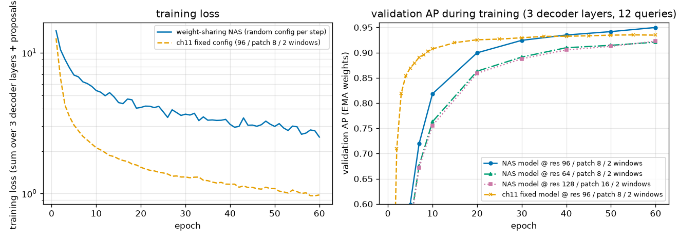
What to read from the training log and Figure 12-5:
- Every combination was trained evenly. The 7,500 steps went to the 23 combinations 300 – 372 times each. The default configuration (96 / 8 / 2 windows) got 335, 4.5% of the total. The fixed-configuration model spent all 7,500 steps on this configuration.
- NAS training is slower early on. The default configuration's AP at epoch 10 is 0.8184 (0.9074 for the fixed-configuration model). That is natural, since the weights must fit inputs of 23 shapes at once.
- But it catches up around epoch 40 and pulls ahead by the end. At epoch 30 it is 0.9244 vs. 0.9294, at epoch 40 0.9349 vs. 0.9325, and at epoch 60 0.9498 vs. 0.9347. The fixed-configuration model plateaued at 0.933 – 0.935 after epoch 40 (chapter 11), while the NAS model is still rising at epoch 60. And this is despite training directly on the default configuration only about 1/22 as much.
- The training loss is much larger on the NAS side (2.52 vs. 0.98 at the last epoch). However, the two cannot be compared directly, because the NAS figure is an average that includes hard configurations such as a 4×4 grid. A comparison on the same configuration is in the "generalization gap" table later.
- It works on other configurations too. In the final scorecard, the NAS model scores 0.9208 at resolution 64, 0.9567 at resolution 128, and 0.9210 at patch 12, which it has never seen. The fixed-configuration model scores 0.1329, 0.3063, and 0.1203 on the same configurations. (The fixed-configuration model's default AP here is 0.9345, which differs by 0.0002 from the 0.9347 in chapter 11's log. This is floating-point error from a different batch size when grouping images for scoring.)
- With 0 decoder layers (encoder proposals only), the NAS model is actually lower (0.8031 vs. 0.8928). This is not what one would expect, and it is examined separately later.
- Training time was the same (949 s; chapter 11's fixed-configuration training took 964 s, both measured while sharing the GPU with other runs). The number of steps is the same, and for this small model step time depends more on the number of operation calls than on the number of tokens. The "2 – 4 times the non-NAS baseline" mentioned in the paper refers to the training length needed to reach the same quality; this experiment held the length equal.
Search: measuring every configuration
With the trained weights, all 408 configurations are evaluated. There is no retraining. Two tricks cut the time.
- One forward pass yields the outputs of the 0- to 3-decoder-layer models at once. The encoder proposals are the output of the 0-layer model, the auxiliary outputs are those of the 1- and 2-layer models, and the final output is that of the 3-layer model. This directly exploits the fact that "the decoder-layer knob has no tie". So forward passes are needed only for the \(34 \times 3 = 102\) combinations of (resolution, patch, windows, number of queries).
- AP computation is split across multiple processes. At this size, chapter 3's
evaluate_apis slower than the forward pass (1 – 2 seconds per configuration).
code/ch12_nas.py · grid-search
def grid_search(model, val_set, device, space, workers: int = 0) -> dict:
    """탐색 공간의 모든 구성에서 검증 AP 를 잰다 (재학습 없음). 돌려주는 값: {Config: (AP, AP50, AP75)}.

    (해상도, 패치, 윈도, 질의 수) 마다 검증 세트를 한 번만 순전파한다. 그 한 번에서 디코더 0 · 1 · 2 · 3층짜리 모델의
    출력이 모두 나온다: 인코더 제안 = 0층, 보조 출력 = 1 · 2층, 마지막 출력 = 3층 (10장에서 확인한 것처럼 정확히 같다).
    AP 계산(3장의 evaluate_ap)이 순전파보다 느려서, 채점은 여러 프로세스에 나눠 맡긴다 (workers > 0).
    """
    model.eval()
    jobs = []
    for resolution, patch_size, num_windows in backbone_configs(space):
        for num_queries in space["num_queries"]:
            out = predict(model, val_set, device, batch_size=125, size=resolution, patch_size=patch_size,
                          num_windows=num_windows, num_queries=num_queries)
            by_depth = [out["enc_outputs"]] + out["aux_outputs"] + [out]  # 디코더 0, 1, 2, 3층
            for dec_layers in space["dec_layers"]:
                layer = by_depth[dec_layers]
                jobs.append((Config(resolution, patch_size, num_windows, dec_layers, num_queries),
                             layer["pred_logits"].numpy(), layer["pred_boxes"].numpy()))
    if workers > 0:
        with multiprocessing.get_context("spawn").Pool(workers, _worker_init, (len(val_set),)) as pool:
            return dict(pool.imap_unordered(_worker_eval, jobs, chunksize=4))
    _WORKER["targets"] = val_set.targets
    return dict(_worker_eval(job) for job in jobs)
[격자 탐색] NAS 학습 모델 (ch12_nas.pt, 60 에폭): 구성 408개의 검증 AP, 169초
[격자 탐색] 11장 고정 구성 모델 (ch11_rfdetr.pt): 구성 408개의 검증 AP, 165초
  check 구성  64 /  8 / 1 / 1 / 12 을 따로 순전파해 잰 AP 0.909987 = 격자 탐색의 값 0.909987
[연산량] FlopCounterMode, 그림 한 장: 45.4 – 705.6 MFLOPs (기본 구성 348.2), 17초
The same grid is also run on the fixed-configuration model (both models use PI-resize for patch resizing). Compute is the per-configuration count of a single-image forward pass with FlopCounterMode, spanning 45.4 – 705.6 MFLOPs, roughly a 15× range. Since the two models share the same architecture, compute and timing were measured only on the NAS model.
[기본 구성] 해상도 / 패치 / 윈도 / 층 / 질의 | 학습 때 | NAS: AP AP50   AP75   | 고정   | MFLOPs  | 배치 1 ms | 배치 64 ms/장
   96 /  8 / 2 / 3 / 12 | 봄  | 0.9498 0.9966 0.9892 | 0.9345 |   348.2 |  3.07 | 0.156
[전체 요약] 구성 408개 (학습 때 본 조합 276개, 못 본 조합 132개)
  NAS 학습 모델          | AP 평균 0.8469, 중앙값 0.8774, 최소 0.5126, 최대 0.9575 | AP ≥ 0.90 인 구성 170개, ≥ 0.80 321개, < 0.50 0개
  11장 고정 구성 모델       | AP 평균 0.2988, 중앙값 0.1315, 최소 0.0000, 최대 0.9350 | AP ≥ 0.90 인 구성 27개, ≥ 0.80 54개, < 0.50 294개
  NAS 학습 모델의 최고 AP: 128 /  8 / 4 / 3 / 12 → 0.9575
  11장 모델: 학습한 (해상도 96, 패치 8) 인 구성 36개의 AP 평균 0.9167 (최소 0.8855), 그 밖의 구성 372개의 AP 평균 0.2390 (최대 0.8676)
  NAS 모델이 11장 모델보다 AP 가 높은 구성: 393 / 408개. (해상도 96, 패치 8) 구성들에서의 차이 NAS − 고정: 평균 -0.0209, 범위 -0.0946 – +0.0153
  학습 때 본 조합의 AP 평균 0.8347, 못 본 조합 0.8725 (디코더 3층 · 질의 12개만: 0.8894 / 0.9233)
[일반화 간격] 기본 구성, 학습 세트의 앞 500장과 검증 500장 (EMA 모델, 추론 모드)
  모델                | 학습 그림: 손실   AP     | 검증 그림: 손실   AP     | 손실의 차이 (검증 − 학습)
  NAS 학습 모델          |           1.7299 0.9566 |           1.8506 0.9498 | +0.1207
  11장 고정 구성 모델       |           0.7040 0.9971 |           1.6477 0.9345 | +0.9437
From left to right, the table columns are: the configuration; whether its (resolution, patch, windows) was ever sampled during training; the NAS model's AP · AP50 · AP75; the fixed-configuration model's AP; compute; batch-1 latency; and per-image time at batch 64 (both times are the minimum of many measurements). The later tables use the same format.
The Pareto curve
- Figure 12-6: ch12-pareto.png The 408 configurations extracted from the NAS model trained once. Each point is one configuration, and color · marker indicate the number of decoder layers (red ▼ 0 layers, orange ■ 1 layer, green ▲ 2 layers, blue ● 3 layers). The black staircase line and black outlines mark the Pareto frontier. On the left the horizontal axis is compute (MFLOPs); on the right the same points are replotted against batch-1 latency measured on this laptop's GPU.
- (Figure content) Two scatter plots of the NAS model's 408 configurations. The horizontal axis is compute on the left and batch-1 latency on the right; the vertical axis is validation AP. The black staircase line is the Pareto frontier.
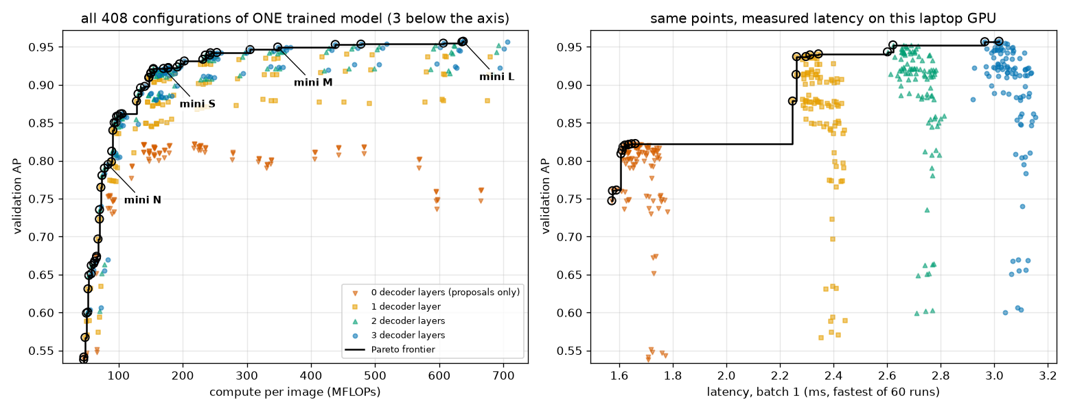
This is the figure promised in chapter 1. Let us read the left panel (compute) first.
- 59 of the 408 lie on the Pareto frontier. The frontier runs from 45 MFLOPs · AP 0.51 to 637 MFLOPs · AP 0.9575. There is a 14× gap between the cheapest and the most accurate configuration, densely filled by 59 points. All of these points came from a single set of weights.
- The frontier is steep at first and flattens later. Up to 100 MFLOPs, a little more compute raises AP sharply (0.51 → 0.86), while beyond 200 MFLOPs doubling the compute raises it by 0.01 – 0.02. How far to go is decided by the budget.
- All five knobs are used. The configurations on the frontier use all nine resolutions, patches 8 · 12 · 16, windows 1 · 2 · 4, decoder layers 0 – 3, and queries 4 · 8 · 12. This matches the first observation in the paper's Appendix L ("every knob is used in the Pareto-optimal family").
- The red points (0 decoder layers) form a separate band at the bottom. Removing the decoder saves little compute (348 → 319 MFLOPs for the default configuration), but AP drops by about 0.15. By compute, 0 decoder layers makes the frontier only for the smallest grids (4×4, 5×5).
- The right panel looks completely different. The same points split horizontally into four clusters (by number of decoder layers), and far fewer points lie on the frontier. This is examined in the section "A frontier that changes with the horizontal axis".
[파레토 경계] 가로축 = MFLOPs: 408개 가운데 59개가 경계 위
  해상도 / 패치 / 윈도 / 층 / 질의 | 학습 때 | NAS: AP AP50   AP75   | 고정   | MFLOPs  | 배치 1 ms | 배치 64 ms/장
   64 / 16 / 1 / 0 /  4 | 봄  | 0.5126 0.7902 0.5815 | 0.0002 |    45.4 |  1.71 | 0.035
   64 / 16 / 1 / 0 /  8 | 봄  | 0.5380 0.8425 0.6053 | 0.0002 |    45.7 |  1.71 | 0.034
   64 / 16 / 1 / 0 / 12 | 봄  | 0.5414 0.8482 0.6095 | 0.0002 |    45.9 |  1.71 | 0.036
  … (가운데 53줄 생략) …
  120 /  8 / 1 / 3 / 12 | 못 봄 | 0.9549 0.9981 0.9865 | 0.4784 |   606.2 |  3.04 | 0.210
  128 /  8 / 2 / 3 / 12 | 봄  | 0.9567 0.9986 0.9899 | 0.3063 |   635.3 |  3.01 | 0.269
  128 /  8 / 4 / 3 / 12 | 봄  | 0.9575 0.9984 0.9898 | 0.3081 |   637.3 |  3.02 | 0.308
    경계 위 구성이 쓰는 resolution: [64, 72, 80, 88, 96, 104, 112, 120, 128]
    경계 위 구성이 쓰는 patch_size: [8, 12, 16]
    경계 위 구성이 쓰는 num_windows: [1, 2, 4]
    경계 위 구성이 쓰는 dec_layers: [0, 1, 2, 3]
    경계 위 구성이 쓰는 num_queries: [4, 8, 12]
Just as the paper picked N · S · M · L from the Pareto frontier, let us set budgets here and pick four. The rule was fixed before looking at the results: the configuration with the highest AP within 1/4 · 1/2 · 1× the default configuration's compute (348.2 MFLOPs), and with no limit.
[미니 N / S / M / L] 연산량 예산 = 기본 구성(348.2 MFLOPs)의 1/4 · 1/2 · 1배 · 제한 없음 안에서 AP 가 가장 높은 구성
  이름 | 예산 MFLOPs | 해상도 / 패치 / 윈도 / 층 / 질의 | 학습 때 | NAS: AP AP50   AP75   | 고정   | MFLOPs  | 배치 1 ms | 배치 64 ms/장
  N    |        87.0 |  80 / 16 / 1 / 3 / 12 | 봄  | 0.7950 0.9636 0.8736 | 0.0001 |    83.6 |  3.11 | 0.061
  S    |       174.1 |  64 /  8 / 4 / 2 / 12 | 봄  | 0.9216 0.9941 0.9813 | 0.1326 |   170.1 |  2.70 | 0.130
  M    |       348.2 |  96 /  8 / 2 / 3 / 12 | 봄  | 0.9498 0.9966 0.9892 | 0.9345 |   348.2 |  3.07 | 0.156
  L    |         inf | 128 /  8 / 4 / 3 / 12 | 봄  | 0.9575 0.9984 0.9898 | 0.3081 |   637.3 |  3.02 | 0.308
  같은 예산에서 11장 고정 구성 모델로 고르면: N 72/12/1/1/4 AP 0.0009, S 64/8/2/2/12 AP 0.1431, M 96/8/2/3/12 AP 0.9345, L 96/8/4/3/8 AP 0.9350
| Name | Configuration (resolution / patch / windows / layers / queries) | Grid | MFLOPs | AP (NAS model) | Fixed-configuration model, same configuration |
| Mini N | 80 / 16 / 1 / 3 / 12 | 5×5 | 83.6 | 0.7950 | 0.0001 |
| Mini S | 64 / 8 / 4 / 2 / 12 | 8×8 | 170.1 | 0.9216 | 0.1326 |
| Mini M | 96 / 8 / 2 / 3 / 12 (default configuration) | 12×12 | 348.2 | 0.9498 | 0.9345 |
| Mini L | 128 / 8 / 4 / 3 / 12 | 16×16 | 637.3 | 0.9575 | 0.3081 |
- The main knob for scaling up is the grid (resolution ÷ patch). From N → S → M → L the grid grows 5 → 8 → 12 → 16. This has the same shape as the paper's N → L, where resolution grows 384 → 704.
- Mini M is exactly chapter 11's default configuration. This means no better configuration existed within that budget.
- Do not read anything into the "4 windows" of mini S · L. On the same grid, the AP difference among 1 · 2 · 4 windows is within 0.001 (e.g., 0.9569, 0.9567, 0.9575 for 128 / 8 / · / 3 / 12). As seen in chapter 11, rerunning the same experiment varies by about this much. The rule of picking the maximum happened to land on it by chance.
- No such family comes out of the fixed-configuration model. Picking by the same budget rule gives N 0.0009, S 0.1431, M 0.9345, L 0.9350. Reducing the budget leaves no usable model, and increasing it brings no improvement.
Extracting from the fixed-configuration model
Here we check: "Couldn't the knobs be turned at inference even if the configuration was never changed during training?" The same 408 configurations are extracted from both models and compared.
- Figure 12-7: ch12-fixed-vs-nas.png Left: for each configuration, the fixed-configuration model's AP (horizontal) and the NAS model's AP (vertical). Points above the diagonal mean the NAS model is higher. Orange squares are configurations with resolution 96 · patch 8, which the fixed-configuration model was trained on, and green stars are configurations never sampled even during NAS training. Middle: AP when changing the inference resolution (1 window, 3 decoder layers, 12 queries). Solid lines are the NAS model, dotted lines the fixed-configuration model, and colors indicate patch size. Right: Pareto frontiers extracted from the two models (horizontal axis compute).
- (Figure content) Left: scatter plot of the fixed-configuration model's AP (horizontal) versus the NAS model's AP (vertical) for the same configurations. Most points lie above the diagonal. Middle: AP by inference resolution. Right: the Pareto frontiers of the two models.
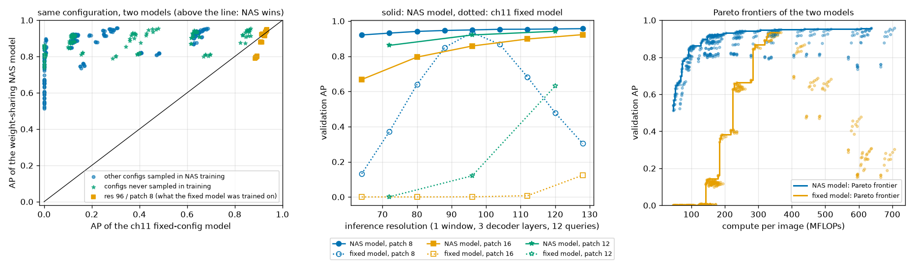
Read the earlier overall summary output together with Figure 12-7.
- The fixed-configuration model works only at the resolution and patch it was trained on. The 36 configurations with resolution 96 · patch 8 average an AP of 0.9167, and the remaining 372 average 0.2390. 294 of the 408 fall short of AP 0.5. The NAS model has none below 0.5, and 321 exceed 0.8.
- It collapses when the resolution moves even slightly (blue dotted line in the middle panel). From 0.935 at 96, it falls to 0.85 · 0.87 at 88 · 104, 0.64 · 0.68 at 80 · 112, and 0.13 · 0.30 at 64 · 128. It is a sharp peak with the training resolution at its summit. The NAS model (blue solid line) stays flat at 0.92 – 0.96 from 64 to 128.
- Patch size is tolerated even less. The fixed-configuration model's AP is near 0 at patch 16 (orange dotted line: below 0.01 up to resolution 112, 0.12 at 128). PI-resize preserves the token values, but when the patch grows, the token grid changes from 12×12 to 6×6 and the number of tokens covering an object drops to 1/4. The later blocks and heads have never seen such input. Compared with the earlier case where enlarging the image and patch together left AP unchanged (the grid stayed at 12×12), this shows that what breaks it is the change in grid, not the patch embedding.
- Some knobs can be turned without training. The orange squares in the left panel (configurations with resolution 96 · patch 8) cluster at 0.89 – 0.94 even for the fixed-configuration model. These 36 configurations differ only in number of windows · decoder layers · queries. This matches the paper treating decoder layers and queries as knobs changed "only at inference", and as seen in chapter 11, a model trained with 2 windows also works as-is with 1 · 4.
- Right panel: the fixed-configuration model's "frontier" is a cliff leading to a single point. Below 300 MFLOPs no configuration exceeds AP 0.85, and above it spending more does not help. The NAS model's frontier lies above it across the entire range.
So far this is as expected. What was not expected is that the NAS model is higher even on the default configuration (0.9498 vs. 0.9345). In the toy problem, sharing weights forced configurations to compromise. Why did the opposite happen? The "generalization gap" table in the output above is a clue. Both models were set to the default configuration, and loss and AP were measured on 500 training images and 500 validation images.
| Model (scored on the default configuration) | Training images: loss | Training images: AP | Validation images: loss | Validation images: AP | Loss gap |
| Fixed-configuration model | 0.7040 | 0.9971 | 1.6477 | 0.9345 | +0.9437 |
| NAS-trained model | 1.7299 | 0.9566 | 1.8506 | 0.9498 | +0.1207 |
- The fixed-configuration model has nearly memorized the training images. Its AP is 0.9971 on training images but 0.9345 on validation images. The loss gap is more than twofold, 0.70 vs. 1.65. This is overfitting. It is what lay behind the observation in chapter 11 that "the training loss kept falling, but validation AP stalled after epoch 40".
- The NAS model has almost no gap. It scores 0.9566 on training images and 0.9498 on validation images. Its score on training images is much lower than the fixed-configuration model's (it did not memorize them), but it is higher on validation images.
This is the typical signature of regularization, pointing in the same direction as the effect the paper calls "architecture augmentation". When the configuration changes every step, it is hard for the weights to memorize the training images in a way that only works on a particular grid. With only 4,000 training images and 1.84 million parameters, this experiment is prone to overfitting, so one can interpret the gain from regularization as outweighing the cost of sharing.
Caution · What this result does not tell us
- It does not separate whether the gain comes from changing the "architecture" or the "resolution". Showing images shrunk and enlarged to various resolutions is itself data augmentation (LW-DETR used it for exactly that purpose). No control experiment varying only resolution while fixing patch · windows was run, so how much of the gain belongs to multi-resolution training is unknown. Chapter 11's fixed-configuration model used no data augmentation at all.
- It cannot be equated with the paper's +0.3 AP. The paper's baseline already uses multi-scale training and augmentation, starts from a pretrained backbone, and trains on COCO. The +0.015 here may mostly be the effect of relieving a small model with no augmentation from overfitting to small data.
- The fixed-configuration model has a single seed. The NAS model's seeds 0 · 1 are close at 0.9498 · 0.9494, but the fixed-configuration model's 0.9347 is a single training run. When the same setting was run for 15 epochs with three seeds in chapter 11, the spread was about 0.005, so a 0.015 difference is larger than that, but the seed spread at 60 epochs was not measured directly.
Let us also compare with other runs. These are the results of running the same grid search on NAS training with a different seed (60 epochs) and on NAS training twice as long (120 epochs).
[다른 실행과의 비교] 같은 격자의 검증 AP
  실행                         | 기본 구성 AP | 기본 구성에서 디코더 0층 | 전체 평균 | 최고   | AP ≥ 0.90 인 구성 | N      S      M      L (위에서 고른 구성의 AP)
  NAS 60 에폭, 시드 0 (본 실행)       | 0.9498       | 0.8031                   | 0.8469    | 0.9575 |  170              | 0.7950 0.9216 0.9498 0.9575
  NAS 120 에폭, 시드 0 (long)      | 0.9596       | 0.8548                   | 0.8761    | 0.9651 |  196              | 0.8401 0.9380 0.9596 0.9651
  NAS 60 에폭, 시드 1 (seed1)      | 0.9494       | 0.8157                   | 0.8452    | 0.9544 |  173              | 0.7960 0.9174 0.9494 0.9522
  11장 고정 구성, 60 에폭             | 0.9345       | 0.8928                   | 0.2988    | 0.9350 |   27              | 0.0001 0.1326 0.9345 0.3081
- Changing the seed gives the same result. Default configuration 0.9498 · 0.9494, overall mean 0.8469 · 0.8452, and 170 · 173 configurations with AP of 0.9 or more. The APs of mini N · S · M · L also agree within 0.006.
- Training longer lifts everything. At 120 epochs, the default configuration is 0.9596 and the overall mean 0.8761, and mini N rose the most, 0.7950 → 0.8401. 60 epochs was not long enough for NAS training. This points in the same direction as the paper budgeting 2 – 4 times the baseline training time and observing on RF100-VL that "architecture augmentation takes more than 100 epochs to converge". (There is no value for the fixed-configuration model trained for 120 epochs. All we know is that its validation AP stalled after epoch 40 in chapter 11.)
- The weakness at 0 decoder layers appears in all three runs (next section).
Sensitivity to each knob
Starting from the default configuration, we turn one knob at a time. This experiment corresponds to the paper's Table 5 · Appendix F.
[손잡이별 민감도] 기본 구성에서 손잡이 하나만 바꾼다
  (resolution) 해상도 / 패치 / 윈도 / 층 / 질의 | 학습 때 | NAS: AP AP50   AP75   | 고정   | MFLOPs  | 배치 1 ms | 배치 64 ms/장
     64 /  8 / 2 / 3 / 12 | 봄  | 0.9208 0.9914 0.9789 | 0.1329 |   160.8 |  3.06 | 0.097
     80 /  8 / 2 / 3 / 12 | 봄  | 0.9423 0.9955 0.9799 | 0.6374 |   243.3 |  3.05 | 0.115
     96 /  8 / 2 / 3 / 12 | 봄  | 0.9498 0.9966 0.9892 | 0.9345 |   348.2 |  3.07 | 0.156   ← 기본
    112 /  8 / 2 / 3 / 12 | 봄  | 0.9537 0.9966 0.9899 | 0.6878 |   477.9 |  3.05 | 0.196
    128 /  8 / 2 / 3 / 12 | 봄  | 0.9567 0.9986 0.9899 | 0.3063 |   635.3 |  3.01 | 0.269
  (patch_size) 해상도 / 패치 / 윈도 / 층 / 질의 | 학습 때 | NAS: AP AP50   AP75   | 고정   | MFLOPs  | 배치 1 ms | 배치 64 ms/장
     96 /  8 / 2 / 3 / 12 | 봄  | 0.9498 0.9966 0.9892 | 0.9345 |   348.2 |  3.07 | 0.156   ← 기본
     96 / 12 / 2 / 3 / 12 | 못 봄 | 0.9210 0.9947 0.9823 | 0.1203 |   169.0 |  3.12 | 0.102
     96 / 16 / 2 / 3 / 12 | 봄  | 0.8573 0.9861 0.9340 | 0.0007 |   112.1 |  3.15 | 0.084
  (num_windows) 해상도 / 패치 / 윈도 / 층 / 질의 | 학습 때 | NAS: AP AP50   AP75   | 고정   | MFLOPs  | 배치 1 ms | 배치 64 ms/장
     96 /  8 / 1 / 3 / 12 | 봄  | 0.9496 0.9965 0.9879 | 0.9350 |   367.4 |  3.01 | 0.150
     96 /  8 / 2 / 3 / 12 | 봄  | 0.9498 0.9966 0.9892 | 0.9345 |   348.2 |  3.07 | 0.156   ← 기본
     96 /  8 / 4 / 3 / 12 | 봄  | 0.9497 0.9992 0.9865 | 0.9348 |   361.0 |  3.05 | 0.188
  (dec_layers) 해상도 / 패치 / 윈도 / 층 / 질의 | 학습 때 | NAS: AP AP50   AP75   | 고정   | MFLOPs  | 배치 1 ms | 배치 64 ms/장
     96 /  8 / 2 / 0 / 12 | 봄  | 0.8031 0.9920 0.9647 | 0.8928 |   318.7 |  1.65 | 0.129
     96 /  8 / 2 / 1 / 12 | 봄  | 0.9351 0.9957 0.9853 | 0.9289 |   329.3 |  2.33 | 0.132
     96 /  8 / 2 / 2 / 12 | 봄  | 0.9443 0.9964 0.9882 | 0.9332 |   338.7 |  2.70 | 0.148
     96 /  8 / 2 / 3 / 12 | 봄  | 0.9498 0.9966 0.9892 | 0.9345 |   348.2 |  3.07 | 0.156   ← 기본
  (num_queries) 해상도 / 패치 / 윈도 / 층 / 질의 | 학습 때 | NAS: AP AP50   AP75   | 고정   | MFLOPs  | 배치 1 ms | 배치 64 ms/장
     96 /  8 / 2 / 3 /  4 | 봄  | 0.9244 0.9849 0.9805 | 0.9163 |   337.4 |  3.05 | 0.148
     96 /  8 / 2 / 3 /  8 | 봄  | 0.9454 0.9963 0.9859 | 0.9342 |   342.8 |  3.07 | 0.156
     96 /  8 / 2 / 3 / 12 | 봄  | 0.9498 0.9966 0.9892 | 0.9345 |   348.2 |  3.07 | 0.156   ← 기본
- Figure 12-8: ch12-knobs.png Validation AP when only one knob is changed from the default configuration (vertical dotted line). The blue solid line is the NAS model, the orange dotted line the fixed-configuration model, and the gray bars (right axis) the compute of each configuration. The panels follow the order (a) – (e) of Figure 3 in the paper.
- (Figure content) Five panels plotting AP as each of the five knobs changes. The NAS model changes gently in every panel, while the fixed-configuration model drops sharply for patch size and resolution.
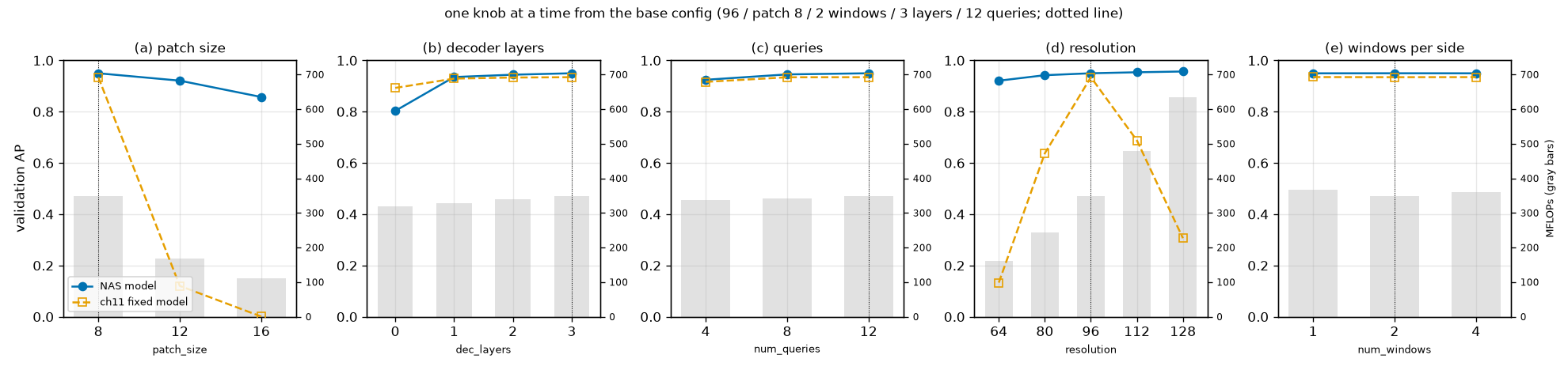
- (a) Patch size: cuts compute the most and lowers AP the most. From 8 → 12 → 16, compute goes 348 → 169 → 112 MFLOPs and AP goes 0.9498 → 0.9210 → 0.8573. Patch 12, never seen during training, falls naturally between 8 and 16.
- (b) Decoder layers: the first layer does most of the work. From 0 → 1 → 2 → 3 layers: 0.8031 → 0.9351 → 0.9443 → 0.9498. Removing the last layer costs −0.0055, removing two costs −0.0147. Each layer accounts for about 10 MFLOPs (3%) of compute; in this mini model the decoder is only 8% of the total. (The paper reports that removing the last layer of Nano on COCO cuts latency by 10% at a cost of 2 mAP. The direction is the same; the magnitude depends on the data and model.)
- (c) Number of queries: nearly unchanged down to 8, drops at 4. From 12 → 8 → 4: 0.9498 → 0.9454 → 0.9244. Even though each image has at most 4 objects, 4 queries are not enough. There is no guarantee that the top 4 cells by encoder score each point to a different one of the four objects (if two cells on one object are both selected, another object is left out). The number of queries needs ample headroom above the maximum number of objects. This is the same lesson as when
num_selectwas reduced in chapter 14. - (d) Resolution: AP rises a little as it goes up, while compute grows quadratically. From 64 → 128, AP goes 0.9208 → 0.9567 and compute 161 → 635 MFLOPs. Objects in the shapes world are large, so the benefit of resolution is small.
- (e) Number of windows: AP stays the same, and compute is smallest with 2 windows. With 1 · 2 · 4 windows, AP is 0.9496 · 0.9498 · 0.9497 and compute is 367.4 · 348.2 · 361.0 MFLOPs. In the earlier hand calculation, 4 windows had the fewest attention pairs, yet total compute is smallest with 2 windows. This is because the per-token computation of the linear layers is proportional to the number of tokens \(N + W^2\) (145 · 148 · 160). With 4 windows, 16 CLS tokens tag along through all six blocks. What the paper's Appendix L says, that "2 windows are usually optimal, and more windows lower efficiency because of CLS token duplication", shows up even in this small model's compute.
- The fixed-configuration model (orange dotted line) keeps up only in (b) · (c) · (e). This is exactly what was seen in the previous section.
What stands out in (b) is 0 decoder layers. The NAS model scores 0.8031 and the fixed-configuration model 0.8928, so only in this configuration is the NAS model lower, by 0.09. The same pattern appears with seed 1 and with 120-epoch training (comparison table above: the 0-layer AP of all three NAS runs is lower than the fixed-configuration model's). AP50 is 0.9920, the same as the fixed-configuration model (chapter 11: 0.9898), so the issue is not failing to find objects but less precise boxes. Moreover, the NAS model's 0-layer AP actually decreases as the grid gets larger (with patch 8 · 1 window · 12 queries: 0.8215 at resolution 64, 0.7614 at 128). Configurations with a decoder attached go the opposite way.
There is a plausible reason (not verified). Encoder proposals must, for each cell of the feature map, predict in one shot "how much to shift and scale the small proposal box centered on that cell" (chapter 10). For the fixed-configuration model, a cell is always 1/12 of the image, but for the NAS model the grid varies from 4×4 to 16×16, so the same head must handle cell sizes differing by a factor of four. Decoder layers re-read the feature map with deformable attention to refine the boxes, so attaching even one layer erases the difference (1 layer: 0.9351 vs. 0.9289). This is an example showing that weight sharing is not free. Some sub-networks lose out because of sharing.
[디코더 층 × 질의 수] 백본 쪽은 기본 구성 (96 / 8 / 윈도 2). 칸: AP (배치 1 지연 시간 ms)
  디코더 층 | 질의  4         | 질의  8         | 질의 12
          0 | 0.7987 (1.66) | 0.8028 (1.66) | 0.8031 (1.65)
          1 | 0.8813 (2.33) | 0.9133 (2.34) | 0.9351 (2.33)
          2 | 0.9215 (2.69) | 0.9426 (2.70) | 0.9443 (2.70)
          3 | 0.9244 (3.05) | 0.9454 (3.07) | 0.9498 (3.07)
This is a mini version of the paper's Appendix B (Figure 4): 12 cells varying the number of decoder layers and queries together, with batch-1 latency in parentheses. The cost of reducing queries is larger the shallower the decoder (1 layer: 0.9351 → 0.8813; 3 layers: 0.9498 → 0.9244). Probably more decoder layers give the queries more chances to divide up roles through self-attention. Latency varies clearly with the number of layers and barely responds to the number of queries. With only 12 queries, there is no computation to save by reducing them (the paper reports that removing 100 of 300 made it "slightly" faster).
Number of spatial locations and unseen configurations
We check Appendix L's claim ("performance follows the number of spatial locations rather than resolution or patch size individually") and Appendix F's claim ("unseen configurations also follow the trend") with the mini experiment. These are 17 configurations with 1 window · 3 decoder layers · 12 queries fixed, varying only (resolution, patch).
[공간 위치 수] 토큰 격자의 한 변 = 해상도 ÷ 패치. 윈도 1, 디코더 3층, 질의 12개
  격자 | (해상도 / 패치: AP, *는 학습 때 못 본 조합) …                                   | AP 의 범위
     4 | 64/16: 0.6677                                                                  |   -
     5 | 80/16: 0.7950                                                                  |   -
     6 | 72/12: 0.8618*, 96/16: 0.8582                                                  | 0.0036
     7 | 112/16: 0.8980                                                                 |   -
     8 | 64/8: 0.9210, 96/12: 0.9209*, 128/16: 0.9228                                   | 0.0019
     9 | 72/8: 0.9315*                                                                  |   -
    10 | 80/8: 0.9411, 120/12: 0.9419*                                                  | 0.0008
    11 | 88/8: 0.9465*                                                                  |   -
    12 | 96/8: 0.9496                                                                   |   -
    13 | 104/8: 0.9532*                                                                 |   -
    14 | 112/8: 0.9536                                                                  |   -
    15 | 120/8: 0.9549*                                                                 |   -
    16 | 128/8: 0.9569                                                                  |   -

[학습 때 못 본 해상도] 패치 8, 윈도 1, 디코더 3층, 질의 12개: 해상도 → AP (*는 못 본 해상도)
  64: 0.9210,  72*: 0.9315,  80: 0.9411,  88*: 0.9465,  96: 0.9496,  104*: 0.9532,  112: 0.9536,  120*: 0.9549,  128: 0.9569
  해상도 72 – 120 가운데 학습 때 본 해상도 3개의 AP 평균 0.9481
  해상도 72 – 120 가운데 학습 때 못 본 해상도 4개의 AP 평균 0.9465
- Figure 12-9: ch12-spatial.png The horizontal axis is the number of spatial locations (side of the token grid = resolution ÷ patch). Blue circles = patch 8, green stars = patch 12, orange squares = patch 16. Hollow markers are (resolution, patch) combinations never sampled during training. Left is validation AP; right is per-image time at batch 64.
- (Figure content) Left: validation AP by side length of the token grid. Points overlap when the grid is the same, even with different patch sizes. Right: per-image time at batch 64 by grid side length.
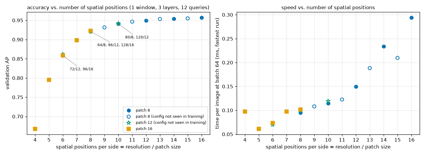
- The same grid gives the same AP. The three ways of making an 8×8 grid (64/8, 96/12, 128/16) score 0.9210, 0.9209, and 0.9228, a spread of 0.0019. The two ways of making a 6×6 grid score 0.8618 · 0.8582, and the two ways of making a 10×10 grid score 0.9411 · 0.9419. This holds even though the resolution differs by a factor of two (64 vs. 128). By contrast, raising the grid one step from 8 to 10 adds 0.02. In the left panel of Figure 12-9, the three marker types overlap on a single curve.
- Patch 12 lies on that curve even though it was never seen during training (green stars). This is the same result the paper confirmed with the unseen patches 27 · 18.
- Unseen resolutions also connect the gaps smoothly. With patch 8, AP from resolution 64 → 128 rises monotonically: 0.9210, 0.9315, 0.9411, 0.9465, 0.9496, 0.9532, 0.9536, 0.9549, 0.9569 (* marks unseen resolutions), and the unseen values sit exactly between the seen ones. The search space behaves not as sparse points but as a continuum.
- As the grid shrinks, AP falls faster and faster. From 16 → 12 it drops −0.007, from 12 → 8 −0.029, and from 8 → 4 −0.25. In a 4×4 grid, one token covers 1/16 of the image, and small shapes are smaller than a single token.
- Speed follows the grid too (right panel). Per-image time at batch 64 is determined by grid size regardless of patch size (different markers overlap at grids 6 · 8 · 10). This matches what was seen with the untrained model in chapter 10. Why the points for grids 4 and 15 stick out from their neighbors was not investigated.
Note · The figure "unseen combinations have a higher average AP". The overall summary output has a line saying "average AP of combinations seen during training 0.8347, unseen combinations 0.8725". This does not mean unseen configurations do better. The seen combinations include small grids such as 4×4 · 5×5 (patch 16), while the unseen combinations are all grid 6 or larger, so their average comes out higher. The table above, comparing like grids, is the correct comparison.
This observation is very useful. What needs to be searched effectively shrinks from the two dimensions of (resolution, patch) to the single dimension of grid size. And among the several ways to make the same grid, the choice can be made on criteria other than accuracy (preprocessing cost, the input size the hardware prefers, or mask detail for segmentation).
A frontier that changes with the horizontal axis
So far compute has been the horizontal axis. Now let us look at the same 408 configurations in terms of time actually measured on this laptop's GPU.
[시간] 구성을 재는 스레드: 성능 코어 3번에 묶음
[시간] 배치 1: 구성마다 60번 (라운드 20 × 3, 번갈아), 103초. 중앙값 1.69 – 6.09 ms (기본 구성 5.91), 최솟값 1.57 – 3.15 ms (기본 구성 3.07)
  기본 구성의 60번: 최소 3.07, 10% 3.12, 25% 5.87, 중앙값 5.91, 75% 5.96, 90% 6.01 ms
  기본 구성의 라운드별 평균 (ms): 6.0 5.9 3.1 6.0 5.9 3.1 5.9 3.1 3.1 6.0 5.9 5.9 5.9 5.9 6.0 5.9 5.9 6.0 5.9 5.9
  구성마다의 '중앙값 ÷ 최솟값': 중앙값 1.93, 최소 1.02, 최대 1.95. 이 비가 1.3 보다 작은 구성 20개, 큰 구성 388개
  → 같은 구성의 값이 빠른 무리와 느린 무리로 갈린다 (중앙값이 어느 무리에 떨어지는지는 구성마다 다를 수 있다). 지연 시간의 대푯값으로 최솟값을 쓴다
[시간] 배치 64: 구성마다 16번, 65초 ('중앙값 ÷ 최솟값' 의 중앙값 1.11, 최대 1.90; 여기서도 최솟값을 쓴다). 그림 한 장당 0.034 – 0.316 ms (처리량 초당 3,165 – 29,038장), 기본 구성 0.156 ms (초당 6,430장)
  디코더 층 수별 (그 층 수인 구성들의 중앙값과 범위): 0층 배치 1 1.68 ms (1.57 – 1.78) · 배치 64 0.093 ms/장, 1층 배치 1 2.35 ms (2.25 – 2.44) · 배치 64 0.103 ms/장, 2층 배치 1 2.71 ms (2.60 – 2.81) · 배치 64 0.107 ms/장, 3층 배치 1 3.06 ms (2.92 – 3.15) · 배치 64 0.111 ms/장
  연산량(MFLOPs)과의 순위 상관(스피어만): 배치 1 지연 시간 -0.102, 배치 64 장당 시간 +0.909 | 디코더 층 수와의 순위 상관: 배치 1 +0.968, 배치 64 +0.180
  GPU 메모리 최대 사용 256 MiB
[기계 상태] load average 3.4 (CPU 코어 16개), GPU 사용률 · 메모리 94 %, 919 MiB, GPU 를 쓰는 프로세스 1개 (이 프로세스 포함)
저장: ch12_search.json  |  측정 전체 873초
- Figure 12-10: ch12-latency.png Top left: times of the first 40 forward passes in the process (log axis). Top middle: distributions of the default configuration's time measured four ways (box = 25 – 75%, horizontal line = median). Top right: histogram of 60 measurements of the default configuration; the red line is the minimum and the black dotted line the median. Bottom left · middle: per-configuration compute (horizontal) versus batch-1 latency · per-image time at batch 64 (vertical); color is the number of decoder layers. Bottom right: time by grid size (relative to the smallest grid, set to 1).
- (Figure content) Six panels. Top: times of the process's first forward passes, box plots of time by measurement method, and a histogram of 60 measurements of the default configuration. Bottom: batch-1 latency versus compute, per-image time at batch 64 versus compute, and relative time by grid size.
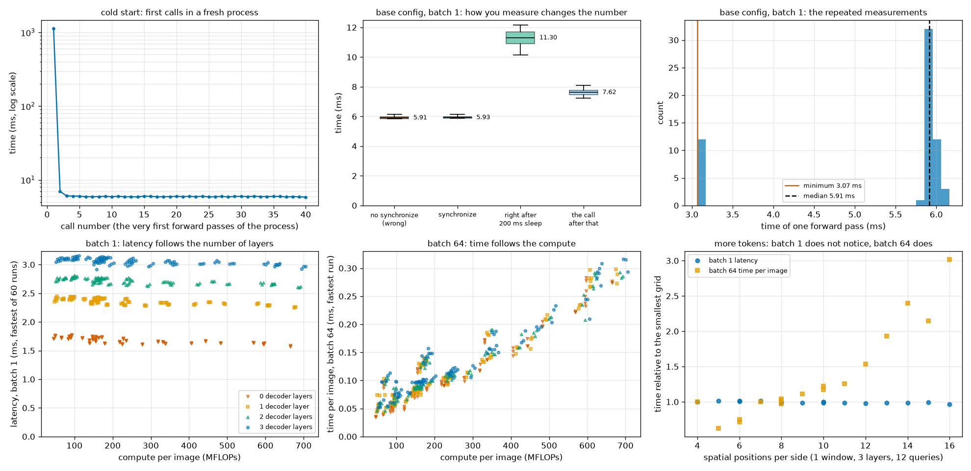
- The histogram (top right) has two peaks. Of the default configuration's 60 measurements, 12 (4 of 20 rounds) are near 3.1 ms and the rest near 5.9 ms. The median is 5.91 ms and the minimum 3.07 ms. For 20 of the 408 configurations, the median fell on the fast side. Had they been ranked by median, these 20 would have looked twice as fast for no reason. With the minimum, configurations with the same number of decoder layers cluster within a band of a little over 0.2 ms.
- Batch-1 latency is determined by the number of decoder layers (bottom left). 0 · 1 · 2 · 3 layers split into four rows at 1.68 · 2.35 · 2.71 · 3.06 ms, and within each row it is flat whether compute is 45 MFLOPs or 700 MFLOPs. The rank correlation between latency and number of decoder layers is +0.968, and with compute −0.102. A 15× difference in compute does not show up in time.
- Per-image time at batch 64 follows compute (bottom middle), with a rank correlation of +0.909. It spans 0.034 – 0.316 ms, a 9× range, or 3,165 – 29,038 images per second in throughput. Here the number of decoder layers barely shows (rank correlation +0.180).
- Batch 1 does not notice more tokens (bottom right). Growing the grid from 4×4 to 16×16 (16× tokens, 11× compute) triples per-image time at batch 64 (0.098 → 0.294 ms), but batch-1 latency stays the same (3.07 → 2.96 ms).
Why this difference? When this mini model runs one image at a time in PyTorch, the GPU sits idle most of the time. What takes the time is the CPU following the Python code and issuing GPU operations one by one, and that cost is proportional not to the size of the operations but to their number. Whether there are 144 tokens or 256, the number of operations issued is the same, while removing one decoder layer eliminates dozens of that layer's operations entirely. This is the same phenomenon as the "GPU latency" changing when the CPU core was switched in the earlier section. At batch 64 each operation becomes large, so the GPU's compute time becomes visible, and only then does compute determine the time.
This is exactly why the paper turned on TensorRT's CUDA graphs. Lining up the kernels in advance removes "the cost of the CPU issuing them one by one", so latency reflects the actual amount of computation more faithfully. In the paper's T4 measurements, lowering the resolution from 640 to 576 cut latency from 4.7 to 4.0 ms (Table 5). There, the number of tokens does show up in latency.
This difference changes the Pareto frontier. Here is the frontier extracted with batch-1 latency as the horizontal axis.
[파레토 경계] 가로축 = 배치 1 ms: 408개 가운데 21개가 경계 위
  해상도 / 패치 / 윈도 / 층 / 질의 | 학습 때 | NAS: AP AP50   AP75   | 고정   | MFLOPs  | 배치 1 ms | 배치 64 ms/장
  128 /  8 / 1 / 0 /  4 | 봄  | 0.7473 0.9812 0.9021 | 0.1513 |   664.6 |  1.57 | 0.275
  128 /  8 / 1 / 0 /  8 | 봄  | 0.7606 0.9937 0.9156 | 0.1631 |   664.9 |  1.57 | 0.274
  128 /  8 / 1 / 0 / 12 | 봄  | 0.7614 0.9936 0.9155 | 0.1643 |   665.2 |  1.59 | 0.277
   88 /  8 / 1 / 0 /  8 | 못 봄 | 0.8094 0.9884 0.9613 | 0.6773 |   277.6 |  1.61 | 0.105
   80 /  8 / 1 / 0 /  4 | 봄  | 0.8137 0.9837 0.9520 | 0.3981 |   224.6 |  1.61 | 0.090
   80 /  8 / 1 / 0 /  8 | 봄  | 0.8185 0.9899 0.9590 | 0.4076 |   224.9 |  1.61 | 0.092
   72 /  8 / 1 / 0 / 12 | 못 봄 | 0.8207 0.9871 0.9442 | 0.1623 |   179.3 |  1.62 | 0.083
   64 /  8 / 1 / 0 /  8 | 봄  | 0.8213 0.9838 0.9490 | 0.0070 |   139.3 |  1.63 | 0.072
   64 /  8 / 1 / 0 / 12 | 봄  | 0.8215 0.9834 0.9495 | 0.0071 |   139.6 |  1.63 | 0.073
   80 /  8 / 2 / 0 /  8 | 봄  | 0.8224 0.9900 0.9619 | 0.4069 |   217.9 |  1.65 | 0.099
   80 /  8 / 2 / 0 / 12 | 봄  | 0.8227 0.9899 0.9621 | 0.4075 |   218.1 |  1.66 | 0.096
  128 /  8 / 1 / 1 /  4 | 봄  | 0.8787 0.9749 0.9635 | 0.2171 |   675.0 |  2.25 | 0.298
  128 /  8 / 1 / 1 /  8 | 봄  | 0.9137 0.9792 0.9723 | 0.2530 |   677.2 |  2.26 | 0.273
  128 /  8 / 1 / 1 / 12 | 봄  | 0.9372 0.9961 0.9871 | 0.2808 |   679.4 |  2.26 | 0.289
  128 /  8 / 2 / 1 / 12 | 봄  | 0.9374 0.9959 0.9874 | 0.2793 |   609.1 |  2.30 | 0.267
  112 /  8 / 1 / 1 / 12 | 봄  | 0.9395 0.9952 0.9880 | 0.6597 |   495.0 |  2.31 | 0.216
  112 /  8 / 2 / 1 / 12 | 봄  | 0.9408 0.9952 0.9878 | 0.6649 |   455.6 |  2.34 | 0.177
  128 /  8 / 1 / 2 /  8 | 봄  | 0.9435 0.9927 0.9885 | 0.2463 |   688.7 |  2.60 | 0.283
  128 /  8 / 1 / 2 / 12 | 봄  | 0.9526 0.9983 0.9899 | 0.2741 |   692.5 |  2.62 | 0.286
  128 /  8 / 1 / 3 / 12 | 봄  | 0.9569 0.9985 0.9899 | 0.3038 |   705.6 |  2.96 | 0.294
  128 /  8 / 4 / 3 / 12 | 봄  | 0.9575 0.9984 0.9898 | 0.3081 |   637.3 |  3.02 | 0.308
    경계 위 구성이 쓰는 resolution: [64, 72, 80, 88, 112, 128]
    경계 위 구성이 쓰는 patch_size: [8]
    경계 위 구성이 쓰는 num_windows: [1, 2, 4]
    경계 위 구성이 쓰는 dec_layers: [0, 1, 2, 3]
    경계 위 구성이 쓰는 num_queries: [4, 8, 12]
- The configurations on the frontier dropped from 59 to 21, all with patch 8. Not one of the patch 12 · 16 configurations, which made up half of the compute-based frontier, remains. The only configurations with 1 or more decoder layers are at resolutions 112 · 128.
- The reason is simple. In this measurement, adding tokens is free. If it is free, using the largest grid always pays off, and every configuration with a smaller grid becomes a dominated point that is "less accurate in the same time". The only knob that reduces time is the number of decoder layers, so the frontier forms four steps following 0 → 1 → 2 → 3 decoder layers (Figure 12-6, right). Lower resolutions appear only on the 0-decoder-layer step, because, as seen earlier, the NAS model's 0-layer AP is lower at higher resolutions.
- Do not read anything into the order within a step. The latencies of configurations with the same number of decoder layers lie within a band of a little over 0.2 ms, and differences within it are indistinguishable from measurement noise. Making the frontier does not mean a configuration is the "fastest" on its step.
Key point · The Pareto frontier is not a property of the model alone. Same weights, same 408 configurations, same AP, yet switching the horizontal axis from compute to this PC's batch-1 latency changed the list of "good configurations". The Pareto frontier is a property of model + hardware + execution method. That is why the paper pinned down the conditions (a TensorRT FP16 engine on a T4), standardized the measurement procedure, and spent 10,000 GPU hours on the search measuring the actual latency of each configuration. This is also where the practical value of weight-sharing NAS lies. When the deployment device changes, you keep the AP as-is, re-measure only the latency, and extract the frontier again. No retraining is needed.
A mini check of fine-tuning after NAS
Finally, let us put the question from the paper's Appendix G to a mini experiment. Once a configuration on the Pareto frontier is picked, does training a bit more on that configuration alone make it better? Starting from the NAS model's EMA weights, we train 10 more epochs (same learning rate and other settings, a single run with seed 0). Four variants are compared.
- Control: continue NAS training as-is for 10 more epochs (configurations still random). This isolates "the effect of simply training longer".
- Fixed to one configuration: 10 epochs fixed to each of the smallest grid (64 / 16 / 1 window, 4×4 grid), a middle one (64 / 8 / 2 windows, 8×8 grid), and the default configuration (96 / 8 / 2 windows, 12×12 grid).
[NAS 뒤 미세 조정] ch12_nas.pt 의 EMA 가중치에서 출발해 10 에폭 더 학습 (학습률 등은 그대로, 시드 0)
  NAS 를 계속 (대조군)         학습 끝 (130초)
  64/16/w1 로 고정          학습 끝 (138초)
  64/8/w2 로 고정           학습 끝 (114초)
  96/8/w2 로 고정           학습 끝 (106초)
  채점하는 구성 →            | 64/16/w1         | 64/8/w2          | 96/8/w2
  미세 조정 전 (NAS 모델)     | 0.6677           | 0.9208           | 0.9498
  NAS 를 계속 (대조군)             | 0.6883 (+0.0205) | 0.9285 (+0.0077) | 0.9520 (+0.0022)
  64/16/w1 로 고정              | 0.7210 (+0.0533) | 0.5974 (-0.3235) | 0.5229 (-0.4269)
  64/8/w2 로 고정               | 0.1558 (-0.5119) | 0.9282 (+0.0074) | 0.8416 (-0.1082)
  96/8/w2 로 고정               | 0.0087 (-0.6591) | 0.5912 (-0.3297) | 0.9582 (+0.0084)
  (괄호 = 미세 조정 전과의 차이. 대각선 — 고정한 구성과 채점하는 구성이 같은 칸 — 이 '그 구성만으로 미세 조정' 의 효과다)
전체 517초
The rows of the table are "how the extra training was done" and the columns are "which configuration it was scored on" (3 decoder layers · 12 queries). The diagonal shows the effect of fine-tuning, and it must be compared against the control row.
- The middle configuration (64 / 8) gains nothing. Fixed fine-tuning gives +0.0074 and the control +0.0077. Fixing the configuration or continuing to mix makes no difference.
- The default configuration (96 / 8) is 0.006 above the control (+0.0084 vs. +0.0022). The direction is a gain, but it is the same size as the run-to-run variation seen in chapter 11 (around 0.005), so with a single seed it is hard to say there is a gain.
- The smallest configuration (64 / 16) rises noticeably (+0.0533, control +0.0205). The 4×4 grid is the sub-network farthest from the other configurations, which fits the picture from the toy problem in exercise 5: "the farther a configuration's preferred value is from the others, the more it compromises because of sharing".
- A fine-tuned model is no longer a family. Look at the off-diagonal cells. Fixing to 96 / 8 and training 10 more epochs collapses 64 / 8 from 0.9208 → 0.5912 and 64 / 16 from 0.6677 → 0.0087. In just 10 epochs it ends up in the same position as the fixed-configuration model. Fine-tuning is a choice to give up the family obtained from one training run in exchange for a single model.
Compared with the paper's observations, the direction is the same. On COCO the fine-tuning gain was +0.4 AP for N and 0.0 – 0.1 AP for S – L, visible only slightly in the smallest model. The result of this mini experiment does not contradict the paper's statement that "fine-tuning is optional". Note, however, that here the control (more NAS training) was also still rising, so this comparison was made while 60 epochs of NAS training had not yet converged.
What this experiment does and does not tell us
Here is what the mini experiment confirmed, side by side with the paper's claims.
| Paper's claim (COCO · RF100-VL) | This chapter's mini experiment (shapes world) | Verdict |
| One training run yields every model on the Pareto curve | 321 of 408 configurations reach AP 0.8 or higher. A frontier spanning a 14× compute range comes from a single set of weights | Same pattern |
| Training with NAS also improves the base configuration (+0.3 AP, architecture augmentation) | Default configuration 0.9345 → 0.9498 (consistent across 2 seeds). Generalization gap shrinks from 0.94 → 0.12 | Same direction. Not separated from the effect of multi-resolution augmentation |
| Decoder layers · queries can be reduced at inference only | Decoder layer · query · window knobs work even on the fixed-configuration model | Same pattern |
| Performance follows the number of spatial locations (resolution ÷ patch) | AP differences among configurations with the same grid are 0.004 or less | Same pattern (even clearer) |
| Configurations not seen during training also follow the trend | 4 unseen resolutions · unseen patch 12 fall on the curve | Same pattern |
| 2 windows are usually optimal (because of CLS duplication) | AP independent of the number of windows; compute smallest with 2 windows | Confirmed on the compute side only |
| Fine-tuning after NAS brings almost no gain (a little only for small models) | A clear gain only for the smallest configuration | Same direction (1 seed) |
| (Not in the paper) | With 0 decoder layers, the NAS model is 0.09 lower than the fixed-configuration model | A sub-network where the cost of weight sharing shows |
And here is what this experiment cannot tell us.
- The magnitudes. The shapes world has large objects and simple backgrounds. That halving the resolution lowers AP by only 0.04 is a property of this data. On COCO, the effect of each knob is much larger.
- The relationship with a pretrained backbone. The paper's model starts from DINOv2 and converts a patch embedding pretrained at patch 14 to other sizes. The mini model started from random initialization.
- Conclusions about latency. Values measured with PyTorch on this PC have entirely different bottlenecks from a TensorRT engine on a T4 (see the section "A frontier that changes with the horizontal axis" above). Which configuration is actually fast can only be known by measuring in the deployment environment.
- Overfitting to the validation set used for search. Picking the maximum out of 408 biases the picked value optimistically. The paper itself mentions the risk of the practice of selecting models on the COCO validation set and reporting on the same set. This chapter did not re-score the selected configurations on a test set. Rankings at the 0.001 level (such as which of 1 · 2 · 4 windows is best) should not be read into.
Connecting to practice
Here is where what this chapter covered shows up when using the actual RF-DETR.
- The released N · S · M · L are configurations found exactly this way. Printing the settings of
RFDETRNano,RFDETRSmall… in chapter 14 shows the values of Table 7 as-is (Nano: resolution 384, patch 16, 2 windows, 2 decoder layers, 300 queries). The backbone of all four sizes is the same DINOv2-S; only the resolution and number of decoder layers differ. The repository's README also states that "the released RF-DETR sizes were produced by neural architecture search". However, the released checkpoints are separate files per size, and this tutorial could not confirm whether those weights are slices of a single shared set of weights or went through per-configuration fine-tuning. - The public package has no NAS training code. The
rfdetrrepository examined by this tutorial did not include a training loop that samples configurations per step or the patch embedding transform. Patch size · number of decoder layers · number of queries are fixed when the model is built. What remains is multi-resolution training (chapter 11: changing the resolution per batch). - So the resolution knob works on actual models too. When the Nano fine-tuned in chapter 14 (training resolution 384) was scored with only the inference resolution changed, AP was 0.9566 at 192, 0.9810 at 256, 0.9830 at 384, and 0.9833 at 640, which was never used. This contrasts with this chapter's fixed-configuration model, which collapsed when the resolution moved even slightly. The difference is whether it experienced multiple resolutions during training. The constraint that the resolution must be a multiple of
patch_size × num_windows(= 32) is the same as this chapter'sis_valid. -
num_selectis not the query knob. In chapter 14, reducingnum_selectfrom 300 to 20 left AP unchanged (0.9830), while reducing it to 2 collapsed it to 0.7116. The lesson that "it needs ample headroom above the maximum number of objects" is the same as in this chapter's query experiment, butnum_selectonly reduces post-processing, not the decoder's computation. - Running NAS on your own data. The README says the same NAS method is available on the Roboflow platform, and states that after the paper was published, the platform's NAS training was improved further to "get every size from a single training run, with results better than the public checkpoints and the paper's NAS results". This is the README's description and was not measured by this tutorial. The terms of use (licenses) for NAS-built models and some sizes are also listed separately in the README, so check them before use.
- Measure latency on your own device, the way you will actually run it. In this chapter's measurements, the time for the same configuration varied by nearly 2× depending on the CPU core and the machine's state at that moment. The numbers in the tables (T4, TensorRT, FP16) are values under those conditions. Chapter 14 has a hands-on session measuring actual models with PyTorch · ONNX Runtime.
Summary
- The right model size differs by hardware and data. Instead of designing and training each size separately, weight-sharing NAS trains a single set of weights once so that it works in every configuration of the search space, and then picks out configurations without retraining.
- Model \(i\) dominates \(j\) when \(t_i \le t_j\), \(a_i \ge a_j\), and it is genuinely better in at least one. A model that is not dominated is Pareto optimal, and sorting by cost and keeping only the points that exceed the running maximum of accuracy yields the Pareto frontier.
- The training objective is the average per-configuration loss \(\mathbb{E}_{c}[\mathcal{L}(\theta; c)]\). Uniformly sampling one configuration per step and updating gives a gradient whose expectation equals the gradient of this objective. Sharing weights forces configurations to compromise, but the constantly changing configuration also acts as regularization (architecture augmentation).
- Each of the five knobs reuses the weights for a different reason. Patch size converts the kernel while preserving dot products with PI-resize \(\hat{w} = (R^\top)^{+} w\); decoder layers can be reduced at inference thanks to the loss applied to every layer, and queries thanks to being selected in score order. Resolution interpolates the position embeddings (boxes are in normalized coordinates, so the head stays the same), and windows have no weights, so only the grouping changes.
- Resolution · patch · windows change from training onward, while decoder layers · queries change only at inference. The paper grid-searched 6,468 configurations (11 × 7 × 7 × 3 × 4), and the resulting N – 2XL scale up mainly through resolution and decoder depth. Performance follows the number of spatial locations (resolution ÷ patch) rather than resolution or patch individually.
- Latency depends on how it is measured. You must synchronize, discard warm-up runs, measure many times, and interleave the things being compared. The paper pauses 200 ms between forward passes to avoid power throttling and reports accuracy and latency from the same artifact.
- Mini experiment: the model NAS-trained for the same 60 epochs exceeded AP 0.8 in 321 of 408 configurations, and its default-configuration AP was also higher than the fixed-configuration model's (0.9498 vs. 0.9345). The fixed-configuration model collapsed outside its training resolution and patch. Configurations with the same grid had the same AP within 0.004, and resolutions and patches unseen during training also fell on the trend. On the other hand, with 0 decoder layers the NAS model was 0.09 lower.
- The Pareto frontier of the same configurations ranked by compute differed from the one ranked by this PC's batch-1 latency. The Pareto frontier is a property of model + hardware + execution method, and with weight-sharing NAS only the latency needs to be re-measured when the device changes.
With this chapter, the story of the RF-DETR detector comes full circle: the architecture (chapter 10), training (chapter 11), and how to pull a family of models out of that single training run (this chapter). What remains is the second task the paper builds on the same framework: instance segmentation. Chapter 13 attaches a lightweight segmentation head that produces masks from the dot product of the decoder's query embeddings and a pixel embedding map. Seeing that architecture also explains why the knobs from this chapter behave a little differently in segmentation (the resolution of the mask features is tied to the input resolution, so "the number of spatial locations" alone does not explain it).
Exercises
- 1. Finding the Pareto frontier
- Seven models have the following (latency ms, AP): P (2, 40), Q (3, 52), R (3, 48), S (4, 50), V (5, 53), T (6, 55), U (7, 55). Find the Pareto frontier with "sort, then sweep once", and for each model not on the frontier name one model that dominates it.
- Sorted by increasing latency (higher AP first on ties), the order is P, Q, R, S, V, T, U. Sweep while remembering the maximum so far.
- P 40 → frontier (max 40). Q 52 → frontier (52). R 48 → discard. S 50 → discard. V 53 → frontier (53). T 55 → frontier (55). U 55 → does not exceed 55, so discard.
- The Pareto frontier is P, Q, V, T. R is dominated by Q (same latency, lower AP), S by Q (slower and less accurate), and U by T (same AP, slower).
- (1) \(3 \times 2 \times 3 \times 4 \times 2 = 144\).
- (2) The grid side is \(64/8 = 8\), \(96/8 = 12\), \(128/8 = 16\) for patch 8, and \(64/16 = 4\), \(96/16 = 6\), \(128/16 = 8\) for patch 16. The number of window counts among 1 · 2 · 4 that divide the grid is 8 → 3, 12 → 3, 16 → 3, 4 → 3, 6 → 2 (not divisible by 4), 8 → 3.
- There are \(3 + 3 + 3 + 3 + 2 + 3 = 17\) backbone combinations, multiplied by 4 decoder layer counts × 2 query counts gives \(17 \times 8 = 136\). Eight were removed (the \(1 \times 8\) configurations with 96 / 16 / 4 windows).
- (1) Nano: \(384/16 = 24\), \(24^2 = 576\). Medium: \(576/16 = 36\), \(36^2 = 1{,}296\). The ratio is \(1296/576 = 2.25\) (the side is 1.5×, so \(1.5^2\)).
- (2) Max: \(828/12 = 69\), \(69^2 = 4{,}761\). About 8.3 times Nano.
- (3) \(560/14 = 40\) and \(640/16 = 40\), so both have \(40^2 = 1{,}600\) tokens. The number of spatial locations is the same. In Table 5 this change moved AP 54.6 → 54.4 with latency unchanged at 4.7 ms. This fits the observation that performance follows the ratio of resolution to patch rather than either one alone.
- (1) \(\langle x, w \rangle = 1 \cdot 2 + 3 \cdot 0 = 2\).
- (2) \(z = (R^\top R)^{-1} w = (0.65 \cdot 2,\ -0.15 \cdot 2) = (1.3,\ -0.3)\). \(\hat{w} = Rz = (1.3,\ 0.75 \cdot 1.3 + 0.25 \cdot (-0.3),\ 0.25 \cdot 1.3 + 0.75 \cdot (-0.3),\ -0.3) = (1.3,\ 0.9,\ 0.1,\ -0.3)\).
- (3) \(Rx = (1,\ 0.75 + 0.75,\ 0.25 + 2.25,\ 3) = (1,\ 1.5,\ 2.5,\ 3)\). \(\langle Rx, \hat{w} \rangle = 1.3 + 1.35 + 0.25 - 0.9 = 2\). Equal to the original dot product.
- (4) \(Rw = (2,\ 1.5,\ 0.5,\ 0)\). \(\langle Rx, Rw \rangle = 2 + 2.25 + 1.25 + 0 = 5.5\), and half of that is \(2.75\). Neither is 2.
- Note that the last value of \(\hat{w}\) is negative (\(-0.3\)). The original kernel had no negative values. Unlike interpolation, PI-resize can produce values outside the range of the original values, and the FlexiViT paper also notes that the PI-resize matrix contains negative weights.
- (1) \(J(\theta) = \tfrac{1}{3}\sum_k (\theta - k)^2\), \(\nabla J = \tfrac{2}{3}\big[(\theta - 1) + (\theta - 2) + (\theta - 6)\big] = 2\theta - 6\). It is zero at \(\theta^\star = 3\) (the mean of the three values). The losses are \((3-1)^2 = 4\), \((3-2)^2 = 1\), \((3-6)^2 = 9\), with a mean of \(14/3 \approx 4.67\).
- (2) At \(\theta = 0\) the gradients are \(2(0-1) = -2\), \(2(0-2) = -4\), \(2(0-6) = -12\), and their average is \(-6\), equal to \(2 \cdot 0 - 6\). Whichever configuration is sampled, the direction is the same; only the magnitude differs.
- (3) Trained alone, the loss would be 0 at \(\theta = 6\). The difference from 9 under sharing is "the price of compromising with the other configurations". The farther a configuration's preferred value is from the others, the more it compromises. In real neural networks, with many weights, the compromise can be much smaller, and it can even turn into a gain by preventing overfitting (as happened with the default configuration in this chapter's experiment).
- \(W = 1\): every block has \(65^2 = 4{,}225\) pairs, so \(6 \times 4{,}225 = 25{,}350\) pairs.
- \(W = 2\): \(16 + 1 = 17\) tokens per window. One window block has \(4 \times 17^2 = 1{,}156\) pairs and one global block \((64 + 4)^2 = 4{,}624\) pairs. Total \(4 \times 1{,}156 + 2 \times 4{,}624 = 4{,}624 + 9{,}248 = 13{,}872\) pairs.
- \(W = 2\) is about 55% of \(W = 1\). However, the number of pairs is only the attention computation; the per-token computation of the linear layers is proportional to the number of tokens \(N + W^2\) and actually increases (\(65 \to 68\)). How much total compute drops depends on the relative weight of the two.
- (1) Auxiliary losses. The same head and the same loss are applied to the encoder proposals and to the output of every decoder layer during training, so each layer's output has already been trained to be a prediction on its own. The output of a model stopped at layer \(k\) is exactly the same as the \(k\)-th auxiliary output of the full model.
- (2) Two-stage query selection picks feature-map cells in order of encoder-side class score, so the queries are already ranked. Using only the top \(N'\) amounts to dropping the lowest-scoring ones first. DETR's queries are learned vectors unrelated to the image, with no per-image ranking, so this method cannot be used.
- (3) These two change the shape of the backbone's input (number of tokens, area covered by each token, interpolation of position embeddings), and weights that have seen only one shape do not work on other shapes. Chapter 11's model, trained only at resolution 96 · patch 8, scored AP 0.13 at resolution 64, 0.31 at 128, and 0.00 at patch 16. The NAS-trained model scores 0.92, 0.96, and 0.86 on the same configurations.
- (1) When this small model runs at batch size 1 in PyTorch, the time the CPU spends issuing operations one by one exceeds the time the GPU spends computing. That time is determined not by the number of tokens but by the number of operations (number of layers). So raising the resolution or shrinking the patch to add tokens leaves latency nearly unchanged while only raising AP. It becomes "for the same cost, use a large resolution and a small patch", and every configuration that reduces tokens is dominated. The only knob that reduces latency is the number of decoder layers.
- (2) The Pareto frontier is a property not of the model alone but of model + hardware + execution method. So the search must use values measured on the device that will actually be deployed, with the runtime environment that will actually be used (for the paper, a TensorRT FP16 engine on a T4). With weight-sharing NAS this is cheap: when the device changes, keep the AP as-is, re-measure only the latency, and extract the frontier again.
See also
- RF-DETR:Tutorial
- RF-DETR
- RF-DETR:Review
- DINOv2
- Vision Transformer
- Object detection
- YOLO
- Dropout
- TensorRT
Favorite site
- 12. Weight-Sharing NAS
- RF-DETR: Neural Architecture Search for Real-Time Detection Transformers (Robinson et al., 2025)
- Once-for-All: Train One Network and Specialize it for Efficient Deployment (Cai et al., 2019)
- FlexiViT: One Model for All Patch Sizes (Beyer et al., 2022)