RF-DETR:Tutorial:11-Training
lastmod 2026-11-18created 2026-11-1813 edits
Training RF-DETR is chapter 11 of the RF-DETR tutorial. The architecture assembled in chapter 10 only decides "which function to use"; how to update that function's weights, toward reducing what, and by which rules, has to be decided separately. This chapter writes the full loss of RF-DETR as a single formula and computes it by hand all the way through, then works through the training settings used by the paper and the public code (a constant learning rate, gradient clipping, exponential moving average, layer-wise learning rate decay, simple augmentation) one at a time, with a formula, a hand calculation, and an implementation for each. It then actually trains a mini RF-DETR and reads the results and the ablations. Results that matched expectations and results that did not are both reported as they are. The checkpoint trained here is the starting point for weight-sharing NAS in chapter 12 and for chapter 13.
- Original: 11. Training RF-DETR
- Lab code:
code/ch11_train.py. It contains the loss (RFDETRCriterion), EMA (ModelEMA), parameter groups and the optimizer, and the training loop. The main experiment (60 epochs of training plus analysis) takes about 17 minutes; the ablations and the backbone pretraining experiment run separately. Reading time of the original is about 110 minutes; difficulty ★★★★☆. - Previous: 10. RF-DETR Architecture / Next: 12. Weight-sharing NAS
- What this chapter covers
- The full RF-DETR loss: matching separately for each query group and each layer, then adding three losses, classification (IA-BCE), L1, and GIoU, with coefficients 1, 5, and 2
- Counting the loss terms, and computing a three-query example by hand all the way through to check it against the code
- Why the loss is applied to the encoder proposals and to every decoder layer
- Optimizer settings, gradient accumulation, and training without warmup or a scheduler: a formula showing why a cosine schedule must know the training length in advance
- The formula and a hand calculation for gradient clipping, and what it means when combined with Adam-family optimizers
- Exponential moving average (EMA): deriving the phrase "an average over roughly the last \(1/(1 - d)\) steps", and the decay warmup in the official implementation
- Layer-wise learning rate decay: building the multiplier table for twelve blocks by hand, using the actual formula from the official code
- Augmentation, multi-resolution training, and the pretraining ladder (DINOv2 → Objects365 → target data)
- Reading the training results of the mini RF-DETR and five ablations, and separating what can be concluded from what cannot
After the architecture comes training
What has been built so far fits in one line. An image (B, 3, H, W) passes through the backbone (a ViT mixed with window attention) and the projector to become a feature map; every cell of the feature map produces a proposal box; the \(N\) highest-scoring cells become the decoder's reference boxes; and the decoder layers refine the queries, each layer producing class logits of shape (B, N, K) and boxes of shape (B, N, 4) (\(K\) is the number of classes). The mini model in this chapter has 1,832,707 weights (during training; at inference only the first query group is used, giving 1,675,870). Right now these weights are random.
Training means updating these weights, and that requires deciding three things.
- What to minimize. This is the loss function. It turns how far the predictions are from the ground truth into a single number.
- How to update. This is the optimizer and its settings: the learning rate, the batch size, and the rules for shaping the gradient.
- Where to start and what to show the model. This is the initial weights (pretraining) and data augmentation.
The RF-DETR paper deliberately keeps the second and third of these simple. As seen in chapter 1, the paper's motivating concern is that "training procedures carefully tuned for COCO alone do not transfer well to other data." So the settings listed in the paper's Appendix A are short.
| Item | RF-DETR (paper Appendix A and Section 3) | Where in this chapter |
| Learning rate | 1e-4 (the paper compares this with "4e-4 for LW-DETR") | Optimizer and learning rate |
| Batch size | 128 (same as LW-DETR) | Batch size and gradient accumulation |
| Learning rate warmup | None | No warmup either |
| Learning rate schedule | "Scheduler-free" training without a cosine schedule | A cosine schedule must know where it ends |
| Gradient clipping | 0.1 | Gradient clipping |
| EMA | Used (with an EMA scheduler) | Exponential moving average |
| Layer-wise learning rate decay | 0.8× per layer on the DINOv2 backbone | Layer-wise learning rate decay |
| Augmentation | Horizontal flip and random crop only | Augmentation and multi-resolution |
| Multi-resolution | 0.5–1.5×, per batch (LW-DETR: 0.7–1.4×, per image) | Augmentation and multi-resolution |
| Pretraining | DINOv2 backbone + Objects365 detection pretraining | The pretraining ladder |
The paper does not write out the loss function (it says it extends LW-DETR and only states that the loss is applied to every decoder layer). So the loss here is written as read from the public code (models/criterion.py and models/matcher.py in rfdetr). In this chapter, "the official implementation" refers to this public code, and "the paper" refers to the RF-DETR paper (Robinson et al., ICLR 2026). Where the two differ, the difference is pointed out each time.
What is being minimized
All the parts of the loss were built in earlier chapters. This section builds no new parts; it gathers into one formula in what order and how many times each part is used.
- Chapter 7: the set loss, which pairs predictions and ground truths one-to-one with Hungarian matching and computes the loss on those pairs; auxiliary losses on every decoder layer.
- Chapter 8: sigmoid classification without a ∅ class, a focal-style matching cost, and two-stage query selection (encoder proposals).
- Chapter 9: the IoU-aware BCE loss (IA-BCE) and Group DETR (query groups).
- Chapter 10: the output structure of the model these parts attach to.
Four places where the loss is applied
During training, the mini RF-DETR's output contains four sets of (class logits, boxes) pairs: the output of each of the three decoder layers, and the encoder proposals before they enter the decoder. These four will be called sites. The loss is applied to all four sites in the same way.
Original figure 11-1. The four sites where the loss of the mini RF-DETR (three decoder layers) is applied. Since each site makes different predictions, matching is redone at each site. The flow of the figure is as follows.
- The backbone + projector produce a feature map, and selecting the top \(N\) cells yields the encoder proposals. Decoder layers 1 → 2 → 3 then make predictions in turn, and the output of layer 3 is the output at inference time.
- Each of the four sites (encoder proposals, decoder layers 1, 2, and 3) produces logits and boxes; at each site, matching is done per group, and then the three losses, classification, L1, and GIoU, are applied.
- The "name suffix" is the suffix attached to that site's loss names in the loss dictionary. The encoder proposals get
_enc, decoder layer 1 gets_0, layer 2 gets_1, and the last layer has no suffix (e.g.,loss_ce_enc,loss_ce_0,loss_ce). - All four sites use the same ground-truth boxes and classes.
- Total loss = the sum of (1 · classification + 5 · L1 + 2 · GIoU) over the four sites.
There are two things to read from the figure. First, the lower boxes of the four sites are all identical; no site uses a different loss. Second, the one without a suffix is the last decoder layer, _0 and _1 are the earlier layers (auxiliary losses), and _enc is the encoder proposals. These names appear as-is in the official implementation's training logs (chapter 14), so they are worth remembering.
The loss at one site
Pick one site and write down, step by step, what happens inside it. First, the notation.
- \(B\): the number of images in the batch. \(T\): the number of ground-truth objects in the batch (summed over all images). Ground truths in an image are indexed by \(j\); the class of ground truth \(j\) is \(c_j\) and its box is \(b_j\).
- \(N\): the number of queries in one query group (12 in the mini model, 300 in the official one). \(G\): the number of groups (4 in the mini model, 13 in the official one). During training there are \(G \cdot N\) queries in total. Groups are indexed \(g = 1, \dots, G\).
- \(\hat{p}_i(c)\): the probability query \(i\) assigns to class \(c\) (the sigmoid of the logit). \(\hat{b}_i\): the predicted box of query \(i\). All boxes are normalized \((c_x, c_y, w, h)\).
① Match each group separately. Build a cost matrix between the \(N\) queries of group \(g\) and the ground truths of that image. The cost of cell \((i, j)\) is
\(C_{ij} \;=\; 2\,C_{\text{cls}}(i, j) \;+\; 5\,\lVert \hat{b}_i - b_j \rVert_1 \;+\; 2\,\big(-\operatorname{GIoU}(\hat{b}_i, b_j)\big)\)
where the classification cost \(C_{\text{cls}}\) is the focal form from chapter 8. Abbreviating \(\hat{p} = \hat{p}_i(c_j)\),
\(C_{\text{cls}}(i, j) = \alpha\,(1 - \hat{p})^{\gamma}\,(-\log \hat{p}) \;-\; (1 - \alpha)\,\hat{p}^{\,\gamma}\,\big(-\log(1 - \hat{p})\big), \qquad \alpha = 0.25,\ \gamma = 2\)
The Hungarian algorithm finds the one-to-one assignment with the smallest total cost, and the result is written \(\hat{\sigma}_g\) (sigma hat). \(\hat{\sigma}_g(j)\) is "the index of the query matched to ground truth \(j\) in group \(g\)." Since there are \(G\) groups, each ground truth gets \(G\) matches (one per group). As seen in chapter 7, no gradient flows through the matching; it is used only to decide the pairs.
- Note: the matching-cost coefficients differ from the loss coefficients
- The matching-cost coefficients are (classification 2, L1 5, GIoU 2), and the loss coefficients that appear just below are (classification 1, L1 5, GIoU 2). Only the classification one differs. The classification term of the matching cost is the focal form while that of the loss is IA-BCE, so the formulas differ as well. Both were read from the official implementation's defaults (
set_cost_class=2,cls_loss_coef=1.0). The criterion for choosing pairs and the criterion for updating the weights with the chosen pairs need not be the same.
② Classification loss: IA-BCE. This is the loss derived in chapter 9. The "ground-truth class cell" \((i, c_j)\) of the matched query \(i = \hat{\sigma}_g(j)\) gets a soft target \(t\) between 0 and 1.
\(t = \hat{p}^{\,\alpha}\, u^{\,1 - \alpha}, \qquad u = \operatorname{IoU}(\hat{b}_i, b_j), \qquad \alpha = 0.25\)
\(u\) is how much the current predicted box overlaps the ground-truth box. The target is treated as a constant (gradient stopped). The official implementation raises \(t\) to 0.01 if it is below 0.01. The per-cell loss is as follows.
\(f_{\text{cls}}(i, c) = \begin{cases} -\,t \log \hat{p} \;-\; (1 - t)\log(1 - \hat{p}) & \text{matched cell } (i, c) = (\hat{\sigma}_g(j),\, c_j) \\ -\,\hat{p}^{\,\gamma} \log(1 - \hat{p}) & \text{all other cells}, \quad \gamma = 2 \end{cases}\)
The upper line is BCE with target \(t\) (the "soft target" from chapter 4), and the lower line is BCE with target 0 multiplied by \(\hat{p}^2\). "All other cells" includes every class cell of unmatched queries and the other class cells of matched queries. To restate the key point of chapter 9: the derivative of the upper line with respect to the logit is \(\hat{p} - t\), and it becomes 0 where \(\hat{p} = t = \hat{p}^{\alpha} u^{1 - \alpha}\), that is, \(\hat{p} = u\). The score is pulled toward the box's IoU. Whether this property actually shows up is checked in the experiments later in this chapter.
③ Box losses: L1 and GIoU. For each matched (predicted box, ground-truth box) pair, compute the L1 distance from chapter 2 and \(1 - \operatorname{GIoU}\). The boxes of unmatched queries get no loss.
④ Sum everything and divide by one number. The three losses at site \(\ell\) (ell) are
\(\begin{aligned} \mathcal{L}^{(\ell)}_{\text{cls}} &= \frac{1}{G \cdot T} \sum_{g=1}^{G} \;\sum_{i,\,c} f_{\text{cls}}(i, c) \\ \mathcal{L}^{(\ell)}_{\text{L1}} &= \frac{1}{G \cdot T} \sum_{g=1}^{G} \sum_{j} \big\lVert b_j - \hat{b}_{\hat{\sigma}_g(j)} \big\rVert_1 \\ \mathcal{L}^{(\ell)}_{\operatorname{GIoU}} &= \frac{1}{G \cdot T} \sum_{g=1}^{G} \sum_{j} \Big( 1 - \operatorname{GIoU}\big(b_j,\, \hat{b}_{\hat{\sigma}_g(j)}\big) \Big) \end{aligned}\)
The inner sum on the first line runs over all queries \(i\) of group \(g\) and all classes \(c\) (including all images in the batch), and \(\sum_j\) on the second and third lines runs over all ground truths in the batch. The superscript \((\ell)\) means "computed from the predictions of site \(\ell\), using that site's matching." The official implementation calls the divisor \(G \cdot T\) num_boxes.
The full loss
Letting \(\mathcal{S}\) be the set of sites (encoder proposals + each decoder layer), the full loss is the following single line.
\(\mathcal{L} \;=\; \sum_{\ell \,\in\, \mathcal{S}} \Big( 1 \cdot \mathcal{L}^{(\ell)}_{\text{cls}} \;+\; 5 \cdot \mathcal{L}^{(\ell)}_{\text{L1}} \;+\; 2 \cdot \mathcal{L}^{(\ell)}_{\operatorname{GIoU}} \Big), \qquad \mathcal{S} = \{\text{enc},\ 1,\ 2,\ \dots,\ L_{\text{dec}}\}\)
\(L_{\text{dec}}\) is the number of decoder layers (3 for the mini model, 2 for Nano, 3 for Small, 4 for Medium). What gets backpropagated is this single number \(\mathcal{L}\). Compared with the auxiliary-loss formula in chapter 7, three things have changed: the encoder proposals (\(\text{enc}\)) are now in the sum, the classification loss has changed from softmax cross-entropy to IA-BCE, and the matching and summation are repeated for each group.
Counting the terms
The formula looks long, but counting makes it simple. The number of loss values is (number of sites) × (3 loss types).
| Model | Decoder layers \(L_{\text{dec}}\) | Number of sites \(L_{\text{dec}} + 1\) | Number of loss values | Queries during training \(G \cdot N\) |
| Mini RF-DETR (this tutorial) | 3 | 4 | \(4 \times 3 = 12\) | \(4 \times 12 = 48\) |
| RF-DETR Nano | 2 | 3 | \(3 \times 3 = 9\) | \(13 \times 300 = 3{,}900\) |
| RF-DETR Small | 3 | 4 | \(4 \times 3 = 12\) | \(3{,}900\) |
| RF-DETR Medium | 4 | 5 | \(5 \times 3 = 15\) | \(3{,}900\) |
Nano's 9 match the nine column names that appear in the training logs of the actual rfdetr package in chapter 14: loss_ce, loss_bbox, loss_giou (last layer), loss_ce_0, loss_bbox_0, loss_giou_0 (first decoder layer), and loss_ce_enc, loss_bbox_enc, loss_giou_enc (encoder proposals). The ce in the names is a legacy name from cross-entropy; the actual content is IA-BCE.
The number of groups \(G\) does not change the "number of loss values" in this table. Raising the number of groups to 13 does not multiply the loss names by 13. Groups only increase the number of queries and matches within one site, and the results are combined into three numbers per site. What does grow is the number of matching problems. Training the mini model for one step on a batch of 32 images runs the Hungarian solver (4 sites) × (32 images) × (4 groups) = 512 times.
Normalizing by the number of groups
There is a reason the divisor is \(G \cdot T\) rather than \(T\). The number of matches grows with the number of groups, so dividing by that factor makes the size of the loss independent of the number of groups.
- With several groups, the loss is the average of the per-group losses
- \(\mathcal{L}_{g} \;=\; \frac{1}{T} \sum_{i,\,c \,\in\, \text{group } g} f_{\text{cls}}(i, c)\)
- This is the classification loss that would have been computed for a model with only group \(g\). With one group, the divisor is \(1 \cdot T = T\).
- The definition for \(G\) groups, restated. Since matching happens only within a group, the per-cell losses are the same as when each group is computed separately.
- Split \(\frac{1}{G \cdot T}\) into \(\frac{1}{G} \cdot \frac{1}{T}\) and moved \(\frac{1}{T}\) into the inner sum.
- The expression in parentheses is \(\mathcal{L}_g\) from the first line. The full loss is the average of the per-group losses. The same holds for the L1 and GIoU losses for the same reason.
The lab code checks this numerically before training. Here is the output when 4 images (14 ground truths) are fed to a randomly initialized model.
[손실] 그림 4장 (정답 14개), 학습 모드: 질의 48개 = 12 × 묶음 4
  층 4개 (마지막 층, 앞 층 2개, 인코더 제안) 마다 짝 [56, 56, 56, 56]개 = 정답 14 × 묶음 4,  num_boxes = 56
  loss_ce 0.1228, loss_bbox 0.5585, loss_giou 0.9958, loss_ce_0 0.1229, loss_bbox_0 0.5673, loss_giou_0 1.0030, loss_ce_1 0.1209, loss_bbox_1 0.5568, loss_giou_1 0.9992, loss_ce_enc 0.1258, loss_bbox_enc 0.5604, loss_giou_enc 0.9976
  check 전체 손실 19.6987 = Σ_층 (1·ce + 5·bbox + 2·giou) = 19.6987
  check 마지막 층 loss_ce 0.122831 = 묶음별 loss_ce [0.1168, 0.1269, 0.1295, 0.1181] 의 평균 0.122831
- Each site has 56 matches. The 14 ground truths each get one match in each of the 4 groups, giving \(14 \times 4 = 56\), which is exactly
num_boxes. - Fourth line: multiplying the twelve values by the coefficients 1, 5, and 2 and adding them gives the same total loss, 19.6987.
- Fifth line: computing the classification loss for each group separately gives 0.1168, 0.1269, 0.1295, and 0.1181, whose average \((0.1168 + 0.1269 + 0.1295 + 0.1181)/4 = 0.4913/4 = 0.1228\) equals
loss_cecomputed all at once. This is the last line of the derivation above. - The box losses are large because the model is freshly built.
loss_giounear 1.00 means \(\operatorname{GIoU} \approx 0\), that is, the predicted boxes barely overlap the ground truth. The four sites having similar values also reflects that the decoder has not yet refined anything.
Computing it all by hand
Take one small example and compute it by hand from matching to the full loss: one image, one site, one group (\(G = 1\)), three queries, and two ground truths. The classes are the three of the shapes world (0 circle, 1 square, 2 triangle).
| Circle | Square | Triangle | Box \((c_x, c_y, w, h)\) | |
| Probabilities of query 0, \(\hat{p}_0\) | 0.80 | 0.10 | 0.10 | (0.32, 0.30, 0.20, 0.20) |
| Probabilities of query 1, \(\hat{p}_1\) | 0.10 | 0.10 | 0.60 | (0.70, 0.62, 0.20, 0.30) |
| Probabilities of query 2, \(\hat{p}_2\) | 0.30 | 0.05 | 0.05 | (0.50, 0.50, 0.10, 0.10) |
| Ground truth 0 | Class = circle | (0.30, 0.30, 0.20, 0.20) | ||
| Ground truth 1 | Class = triangle | (0.70, 0.60, 0.20, 0.30) | ||
Because classification is sigmoid-based, the three probabilities of one query need not sum to 1. Query 0 is offset 0.02 to the right of ground truth 0, query 1 is offset 0.02 below ground truth 1, and query 2 is a small box that overlaps neither ground truth.
- Step 1 · Matching cost — cell (query 0, ground truth 0)
- \(\alpha\,(1 - \hat{p})^{\gamma}\,(-\log \hat{p}) = 0.25 \times 0.2^2 \times 0.22314 = 0.00223\)
- The class of ground truth 0 is circle, and the probability query 0 assigns to circle is \(\hat{p} = 0.8\). \(-\log 0.8 = 0.22314\). This is "the focal loss this cell would receive if matched."
- \(-\log 0.2 = 1.60944\). This is "the focal loss this cell would receive if not matched."
- The difference of the two. The higher a cell's probability, the more it gains from being matched, so the cost becomes strongly negative.
- Add the absolute differences of the four coordinates. Only the horizontal center coordinate differs, by 0.02.
- To compute IoU, convert to the corner representation \((x_1, y_1, x_2, y_2)\) by subtracting and adding half the width and height from the center.
- Each box has area \(0.2 \times 0.2 = 0.04\). The union follows from the inclusion–exclusion principle.
- The enclosing box is \((0.20, 0.20, 0.42, 0.40)\) with area \(0.22 \times 0.20 = 0.044\), equal to the union. Two boxes shifted only sideways leave no empty space between them, so GIoU equals IoU.
- Add with the coefficients 2, 5, and 2. The class is right and the box is close, so the cost is strongly negative.
- Step 1 (continued) · Cell (query 2, ground truth 0) and the cost matrix
- \(C_{\text{cls}} = 0.25 \times 0.7^2 \times 1.20397 - 0.75 \times 0.3^2 \times 0.35667 = 0.14749 - 0.02408 = 0.12341\)
- The probability query 2 assigns to circle is \(\hat{p} = 0.3\). The logarithm in the first term is \(-\log \hat{p} = -\log 0.3 = 1.20397\) and the one in the second term is \(-\log(1 - \hat{p}) = -\log 0.7 = 0.35667\); they are different numbers (an easy place to get confused). The probability is low, so the cost is positive, meaning matching would be a loss.
- The coordinate-wise differences between \((0.50, 0.50, 0.10, 0.10)\) and \((0.30, 0.30, 0.20, 0.20)\).
- The corners of query 2 are \((0.45, 0.45, 0.55, 0.55)\), which do not overlap ground truth 0, so \(\operatorname{IoU} = 0\); the union is \(0.01 + 0.04 = 0.05\), and the enclosing box is \((0.20, 0.20, 0.55, 0.55)\) with area \(0.35^2 = 0.1225\).
- All three terms are positive. This cell is unlikely to be matched.
- The remaining four cells are computed the same way (rows = queries 0, 1, 2; columns = ground truths 0, 1). There are \(3 \times 2 = 6\) ways to assign a different query to each of the two ground truths, and the one with the smallest sum is (query 0 ↔ ground truth 0, query 1 ↔ ground truth 1), at \(-3.0770 - 2.1039 = -5.1809\). These are the only two negative cells, so every other assignment is larger. Query 2 has no match.
- Step 2 · Classification loss (IA-BCE)
- \(t_0 = 0.8^{0.25} \times 0.81818^{0.75} = 0.94574 \times 0.86028 = 0.81360\)
- The target for the match (query 0, circle). It blends the score 0.8 and the IoU 0.818 with exponents 0.25 and 0.75. The IoU exponent is larger, so the target is close to the IoU.
- BCE with target \(t_0\). Even though the score 0.80 is almost the same as the target 0.81, the loss is not 0. When the target is strictly between 0 and 1, the minimum of BCE is not 0 (see the box below).
- The target for the match (query 1, triangle). The IoU, computed the same way, is \(0.056 / 0.064 = 0.875\) (intersection \(0.20 \times 0.28\), union \(0.06 + 0.06 - 0.056\)).
- The score 0.6 is below the target 0.80. This cell's gradient \(\hat{p} - t = 0.6 - 0.796 \lt 0\) points toward raising the score.
- The other seven cells: four cells with probability 0.1 (square and triangle of query 0, circle and square of query 1) and the three cells of the unmatched query 2 (0.3, 0.05, 0.05). Since each is \(\hat{p}^2 \cdot (-\log(1 - \hat{p}))\), low-probability cells are nearly 0, and the single 0.3 cell accounts for most of the total.
- Add the losses of all nine cells and divide by
num_boxes\(= 1 \times 2\).
- Step 3 · Box losses and the full loss
- \(\mathcal{L}_{\text{L1}} = \frac{0.02 + 0.02}{2} = 0.02\)
- The L1 distances of the two matches. Query 1 differs only in the vertical center coordinate, by 0.02. The box of the unmatched query 2 is not included.
- For both matches GIoU equals IoU (same-size boxes shifted in only one direction).
- This is the loss of this one site. In the real model the same computation is done at every site (four in the mini model) and everything is added.
These numbers can be checked directly with this chapter's loss class. Run the following from the code/ folder.
Checking the hand-calculation example with RFDETRCriterion
import torch
from ch11_train import RFDETRCriterion

p = torch.tensor([[0.8, 0.1, 0.1], [0.1, 0.1, 0.6], [0.3, 0.05, 0.05]])  # 질의 3개 × 클래스 3개의 확률
outputs = {"pred_logits": torch.log(p / (1 - p))[None],  # (1, 3, 3): 확률을 로짓으로
           "pred_boxes": torch.tensor([[[0.32, 0.30, 0.20, 0.20], [0.70, 0.62, 0.20, 0.30], [0.50, 0.50, 0.10, 0.10]]])}
targets = [{"labels": torch.tensor([0, 2]),  # 원, 삼각형
            "boxes": torch.tensor([[0.30, 0.30, 0.20, 0.20], [0.70, 0.60, 0.20, 0.30]])}]
criterion = RFDETRCriterion(group_detr=1).eval()  # 평가 모드 = 묶음 1개
cost = criterion.matcher.cost_matrix(outputs["pred_logits"][0], outputs["pred_boxes"][0],
                                     targets[0]["labels"], targets[0]["boxes"])
losses, matches = criterion(outputs, targets, return_matches=True)
print("비용 행렬 (질의 3 × 정답 2)\n", cost.numpy().round(4))
print("짝: 질의", matches[0][1].tolist(), "↔ 정답", matches[0][2].tolist())
print({k: round(float(v), 4) for k, v in losses.items()})
비용 행렬 (질의 3 × 정답 2)
 [[-3.077   6.204 ]
 [ 6.4462 -2.1039]
 [ 4.4305  5.0183]]
짝: 질의 [0, 1] ↔ 정답 [0, 1]
{'loss_ce': 0.5558, 'loss_bbox': 0.02, 'loss_giou': 0.1534, 'loss': 0.9626}
The cost matrix, the matches, the three losses, and the full loss all agree with the hand calculation.
- Note: the IA-BCE loss does not go down to 0
- BCE with target \(t\), \(-t\log\hat{p} - (1 - t)\log(1 - \hat{p})\), is smallest at \(\hat{p} = t\), and its minimum is \(-t \log t - (1 - t)\log(1 - t)\). Unless \(t\) is 0 or 1, this value is greater than 0. For example, with \(t = 0.95\) it is \(0.95 \times 0.05129 + 0.05 \times 2.99573 = 0.04873 + 0.14979 = 0.1985\). That is why, in this chapter's training logs, the classification loss (
ce) does not head toward 0 like the box losses, but descends slowly from some height. As the boxes improve and \(t\) approaches 1, this floor also drops. A large loss value does not mean the classification is wrong.
Why the loss is applied at every site
Only the output of the last decoder layer is used at inference. Even so, the loss is applied to the other sites, and the reason differs from site to site.
Why apply it to the encoder proposals
Recall query selection from chapter 10. For every cell of the feature map, the two-stage head produces class logits and a box; the top \(N\) cells by maximum class logit are selected, and their boxes become the decoder's reference boxes. The gradient is cut in two places here.
- The "select the top \(N\)" operation only outputs indices and is not differentiable. There is no gradient with respect to which cells were chosen.
- The selected boxes pass through a stop-gradient before entering the decoder (chapter 8). The gradient of the decoder-side losses does not flow back into the proposal boxes.
The decoder's content queries are separately learned embeddings rather than features of the selected cells, so these two are the only paths to the two-stage head (the proposals' classification head and box head, and the linear layer in front of them). Therefore the decoder-side losses alone do not train the two-stage head at all. If the three encoder-proposal loss terms are removed from the mini model before backpropagation, the gradient of the two-stage head comes out exactly 0 (this was checked separately and is not output by this chapter's code; the backbone, projector, decoder, and heads do receive gradients).
The proposal scores would then stay random, the "top \(N\) cells" would be arbitrary cells, and the decoder would start from places unrelated to the objects. The loss on the encoder proposals is not a bonus; it is the only training signal that makes query selection meaningful. Since that loss is the same as for the decoder layers (matching → IA-BCE, L1, GIoU), the proposals are trained to be "coarse detection results" in their own right. This is why scoring the proposals alone gives a fairly high AP in the experiments later on.
Why apply it to every decoder layer
The losses on the earlier decoder layers are exactly the auxiliary losses of chapter 7, for the same reason. Every layer receives a signal directly from the ground truth, and every layer's output is read by the same heads, so stopping at any layer still yields (class, box) outputs.
RF-DETR uses this property as a design ingredient. Section 3 of the paper states that because the loss is applied to the output of every decoder layer, some or all of the decoder layers can be removed at inference, and it makes the number of decoder layers one of the knobs of weight-sharing NAS. Removing all the layers makes the encoder proposals themselves the prediction, which in the paper's words behaves like an NMS-free single-stage detector. This is where the two losses meet: thanks to the loss on the encoder proposals, "0 decoder layers" also produces usable predictions, and thanks to the per-layer losses, so do "1 decoder layer" and "2 decoder layers." This chapter's experiments measure AP by number of layers; the full story comes in chapter 12.
- Key points · Structure of the loss
- Hungarian matching is done separately for each site (encoder proposals + each decoder layer) and each group. The cost is \(2 \cdot\) focal-style classification \(+\ 5 \cdot\) L1 \(+\ 2 \cdot (-\operatorname{GIoU})\).
- At each site, the three losses (IA-BCE, L1, \(1 - \operatorname{GIoU}\)) are divided by (number of ground truths) × (number of groups) and added with coefficients 1, 5, and 2. The full loss is the sum over all sites.
- The encoder-proposal loss is the only signal that trains query selection, and the per-layer losses make it possible to remove decoder layers.
Optimizer and learning rate
With the loss settled, the next question is "how to update." RF-DETR's answer is short: AdamW, with the same learning rate from start to finish.
AdamW and the basic settings
The optimizer is AdamW from chapter 4. It sets the direction from an exponential moving average of the gradient and a per-parameter step size from an exponential moving average of the squared gradient, and applies weight decay separately from the gradient. Here are the values from three sources side by side.
| Setting | Paper (Appendix A) | Official implementation defaults ( | Mini experiment in this chapter |
| Optimizer | (follows LW-DETR) | AdamW | AdamW |
| Learning rate | 1e-4 | | 2e-4 |
| Base learning rate of the backbone | Not stated | | 3e-4 (same 1.5× ratio) |
| Weight decay | Not stated | | 1e-4 |
| Batch size | 128 | | 32 |
| Epochs | Varies by dataset | | 60 |
| Learning rate schedule and warmup | None | Constant throughout training, | None |
- The learning rate is low. The paper compares it with "4e-4 for LW-DETR" and explains that a low learning rate helps preserve DINOv2's pretrained knowledge (Section 4). Looking at the LW-DETR paper directly, 4e-4 is the value for Objects365 pretraining (6e-4 for the backbone); COCO fine-tuning uses 1e-4 for the projector and decoder and 1.5e-4 for the backbone. The official implementation's defaults
lr=1e-4andlr_encoder=1.5e-4match these numbers. - The mini experiment's learning rate of 2e-4 was chosen to match the experiments in chapter 7 and chapter 8. It is a little larger than the official default because a small model is trained from scratch. It was not chosen by comparing it against other values.
- The paper's batch size of 128 is the authors' large-scale experimental setup, while the official implementation's default is a small value that fits on a single GPU. The mechanism that bridges the gap is gradient accumulation, in the next subsection.
Batch size and gradient accumulation
A larger batch gives a less noisy gradient but uses more GPU memory. Gradient accumulation computes the gradient of a large batch by splitting it into several small batches. Run forward and backward passes on small batches \(A\) times, adding up the gradients without clearing them, and update the weights only once on the \(A\)-th pass. In PyTorch, backward() adds to the gradient rather than overwriting it, so it is enough to call zero_grad() once every \(A\) passes.
- Average gradient over A small batches = gradient of one large batch
- \(\mathcal{L}_{\text{large}} = \frac{1}{A \cdot B} \sum_{k=1}^{A \cdot B} f_k \quad \Rightarrow \quad \nabla \mathcal{L}_{\text{large}} = \frac{1}{A \cdot B} \sum_{k=1}^{A \cdot B} \nabla f_k\)
- The loss of a large batch of \(A \cdot B\) images is the average of the per-image losses \(f_k\). \(\nabla\) (nabla) is the gradient with respect to the weights. The gradient of a sum is the sum of the gradients.
- The gradient obtained by splitting the same images into \(A\) chunks of \(B\) images and backpropagating each chunk separately. The weights are not updated in between, so every \(\nabla f_k\) is computed at the same weights.
- Average the gradients of the small batches (in practice, divide the loss by \(A\), backpropagate, and add up the gradients). The double sum becomes a single sum over all images.
- This equals the first line. The number of images seen per weight update, \(A \cdot B\), is the effective batch size (chapter 14).
In numbers: suppose the gradients of one weight from four images are 0.2, 0.6, 0.5, and 1.1. Computed as one batch of four, the result is \((0.2 + 0.6 + 0.5 + 1.1)/4 = 0.6\). Split into two batches of two, the first gives \((0.2 + 0.6)/2 = 0.4\) and the second \((0.5 + 1.1)/2 = 0.8\), and their average \((0.4 + 0.8)/2 = 0.6\) is the same.
- Caution · Conditions for this equality
- The loss of one image must not depend on the other images in the same batch. Batch normalization uses the batch mean and variance, so it breaks this condition (chapter 4). This is why the RF-DETR paper replaced the batch normalization in the projector with layer normalization. The paper states that this makes it possible to train on consumer GPUs with gradient accumulation (Section 3).
- The RF-DETR loss is divided not by the number of images but by the number of ground truths in the batch (
num_boxes). If the small batches have different numbers of ground truths, the average over several small batches differs slightly from a single large batch. Nearly the same, but not exactly.
The mini experiment in this chapter does not use gradient accumulation, because the model is small enough for a batch of 32 to fit at once.
Learning rate schedulers and the cosine schedule
A mechanism that changes the learning rate during training according to a fixed rule is called a learning rate scheduler. The usual idea is to move fast with a large learning rate at first, then lower it toward the end to settle in finely. The experiments in chapter 7 and chapter 8 also cut the learning rate to 1/10 after 48 of 60 epochs.
The most widely used is the cosine schedule. With \(n\) the number of steps so far, \(n_{\text{end}}\) the total number of training steps, \(\eta_0\) (eta) the initial learning rate, and \(\eta_{\min}\) the final learning rate,
\(\eta_n = \eta_{\min} + \tfrac{1}{2}\,(\eta_0 - \eta_{\min})\left(1 + \cos\frac{\pi\, n}{n_{\text{end}}}\right)\)
(Papers usually write \(n\) as \(t\) and \(n_{\text{end}}\) as \(T\); this chapter avoids those because \(t\) and \(T\) are already used for the loss target and the number of ground truths.) The formula is the same whether counted in steps or epochs.
- Three points on the cosine schedule
- \(n = 0: \quad \cos 0 = 1 \;\Rightarrow\; \eta_0 = \eta_{\min} + \tfrac{1}{2}(\eta_0 - \eta_{\min}) \cdot 2 = \eta_0\)
- At the start the parenthesized factor is 2, so the learning rate is the initial value.
- Exactly halfway, it is the average of the two learning rates.
- At the end the factor is 0, reaching the final learning rate.
- Since \(\cos(\pi/4) = 0.70711\), \(\tfrac{1}{2}(1 + 0.70711) = 0.85355\); since \(\cos(3\pi/4) = -0.70711\), \(\tfrac{1}{2}(1 - 0.70711) = 0.14645\). The curve falls slowly at the beginning and end and quickly in the middle.
A cosine schedule must know where it ends
Looking at the formula again, \(n\) never appears on its own, only as \(n / n_{\text{end}}\). The learning rate is determined not by "which step are we on" but by "what fraction of the whole has passed." So \(n_{\text{end}}\) must be fixed before training starts, and once fixed, it governs the learning rate of every step throughout training.
Original figure 11-2. Three schedules starting from the same initial learning rate \(\eta_0\) (\(\eta_{\min} = 0\)). The horizontal axis is epochs (0–100), and the vertical axis is the learning rate (0–\(\eta_0\)).
- Constant learning rate (RF-DETR): a horizontal line at \(\eta_0\).
- Cosine, end = 100 epochs: starts at \(\eta_0\) and reaches 0 at epoch 100.
- Cosine, end = 50 epochs: starts at \(\eta_0\) and reaches 0 at epoch 50.
- At epoch 30 (vertical dotted line), the learning rate is \(1.00\,\eta_0\) for the constant learning rate, \(0.79\,\eta_0\) for the cosine schedule ending at 100 epochs, and \(0.35\,\eta_0\) for the one ending at 50 epochs. The learning rate at the same epoch 30 depends on where the "end" was set.
The vertical dotted line in the figure is the point. At the same moment, after 30 epochs of training, the learning rate the model is receiving depends on the planned length. The numbers come straight from the formula: with \(n_{\text{end}} = 100\), \(\tfrac{1}{2}(1 + \cos 0.3\pi) = \tfrac{1}{2}(1 + 0.58779) = 0.794\); with \(n_{\text{end}} = 50\), \(\tfrac{1}{2}(1 + \cos 0.6\pi) = \tfrac{1}{2}(1 - 0.30902) = 0.345\). This creates two problems.
- Planned long but want to stop early. Suppose 100 epochs were planned, but the data is small and 30 epochs would have been enough. Stopping at epoch 30 leaves the learning rate still at \(0.79\,\eta_0\), producing a model that never went through the later phase where the lowered learning rate refines it.
- Planned short but want to train longer. Suppose 50 epochs were planned and run to the end, but performance was still improving. The learning rate is already 0, so training cannot simply continue. The length has to be reset and the schedule rebuilt.
If only COCO matters, this is not a problem: run several times and find the right length. But RF-DETR targets real-world datasets of widely varying size and difficulty. Section 3 of the paper puts it this way: the cosine schedule assumes the optimization length is known in advance (fixed), and that assumption does not hold for diverse target data such as the datasets of RF100-VL. The paper adds that this observation was made around the same time as DINOv3.
So RF-DETR does not change the learning rate. With a constant learning rate, the model at epoch 30 is the same whether it is "epoch 30 of a 100-epoch plan" or "epoch 30 of a 50-epoch plan." Training can stop at any time or keep going. The paper calls this scheduler-free training (meaning that the augmentation schedule is also removed, not just the learning rate schedule; augmentation is covered later).
- Note · In the public code
- The official implementation's default schedule is named
lr_scheduler="step"and is set to lower the learning rate after a fixed epoch (lr_drop, default 100). But the default number of epochs is also 100, so under the default settings the learning rate stays constant throughout training. In the actual training run in chapter 14, the learning rate did not change either.
Still, there was a reason for lowering the learning rate. With a large learning rate, the weights keep jittering around a good spot. If the learning rate stays the same to the end, what reduces that jitter? In RF-DETR, the mechanism that can be seen as taking on that job is EMA, introduced below. Rather than making the weights themselves move less, it keeps a separate average of the moving weights and uses that. (This is not how the paper explains it; it is an interpretation comparing the roles of the two mechanisms.)
No warmup either
Warmup gradually raises the learning rate from near 0 to its target value during the first part of training. It came from the concern that a freshly initialized model has large gradients with unreliable directions, so starting with a large learning rate could fling the weights somewhere strange. It is common when training Transformers.
Appendix A of the RF-DETR paper states that learning rate warmup was removed (contrasting it with DINOv3, which uses warmup while RF-DETR does not). The official implementation's default is also warmup_epochs=0. The paper does not explain why. Still, several conditions that make warmup unnecessary can be seen in this chapter: the learning rate itself is low, most weights start from pretrained values rather than random ones, and gradient clipping in the very next section bounds the size of each step. Removing warmup also removes one number that has to be decided in advance (the warmup length).
Gradient clipping
Since chapter 7, the training loop has contained the line clip_grad_norm_(model.parameters(), 0.1). This is gradient clipping, whose explanation was deferred to this chapter.
Clipping by norm
Let \(\mathbf{g}\) be the vector formed by concatenating the gradients of all the model's weights (1,832,707 components for the mini model). Its length, the norm, is \(\lVert \mathbf{g} \rVert = \sqrt{\sum_k g_k^2}\). Gradient clipping shrinks only the length, keeping the direction, down to \(c_{\max}\) whenever the length exceeds a preset limit \(c_{\max}\).
Think of a dog on a leash. Within the leash length (\(c_{\max}\)), it goes as far as it likes. If it tries to go farther, it moves in the direction it wanted but only up to the leash length. The dog chooses the direction; the leash only sets the upper bound on distance.
- Deriving the clipping formula
- \(\mathbf{g}' = s\,\mathbf{g}, \qquad s \gt 0\)
- To preserve the direction, every component must be multiplied by the same positive number \(s\). Multiplying components by different numbers changes the direction.
- The new length must not exceed the limit \(c_{\max}\). Multiplying a vector by \(s\) multiplies its length by \(s\).
- The gradient is never enlarged. A gradient already within the limit must be left as is.
- The largest \(s\) satisfying both conditions. If \(\lVert \mathbf{g} \rVert \le c_{\max}\), then \(s = 1\) (unchanged); otherwise \(s = c_{\max} / \lVert \mathbf{g} \rVert\) and the new length is exactly \(c_{\max}\).
- Hand calculation — a two-component gradient, limit 0.1
- \(\mathbf{g} = (3,\ 4): \quad \lVert \mathbf{g} \rVert = \sqrt{9 + 16} = 5, \qquad s = \min\!\left(1,\ \frac{0.1}{5}\right) = 0.02\)
- The length 5 exceeds the limit 0.1, so it is shrunk.
- The 3 : 4 ratio of the two components is unchanged, and the length is now exactly 0.1.
- A gradient within the limit is not touched. Feeding the same two vectors to PyTorch's
clip_grad_norm_gives \((0.06, 0.08)\) and \((0.03, 0.04)\) (the only difference is that it adds a tiny \(10^{-6}\) to the denominator).
Two points are worth noting. First, there is one norm for the whole model; it is not measured per layer. So when one layer's gradient spikes, the gradients of the other layers are shrunk along with it. Second, Appendix A of the paper says "all gradients larger than 0.1 are clipped," and in the official implementation this value is used as the limit on the total norm under the name clip_max_norm=0.1. The value has been carried over since the DETR paper (chapter 7).
Why it is needed, and what it means with Adam
The original purpose of gradient clipping is to keep a single bad batch from ruining training. This happens often in the DETR family. Matching is redone at every step, so the loss jumps the moment the pairs change, and since the loss is a sum over several sites, the jump stacks up once per site. The gradient at such a step can be several times its usual size.
With SGD the effect is easy to read. The update is \(\eta\,\mathbf{g}\), so after clipping, the distance the weights move in one step cannot exceed \(\eta \cdot c_{\max}\). With the Adam family it has to be read a little differently. As seen in chapter 4, Adam's update is roughly (moving average of the gradient) ÷ (moving average of the gradient magnitude), so multiplying the whole gradient by the same constant every time changes the numerator and denominator together and leaves the update unchanged. So with Adam, gradient clipping is not a mechanism for shrinking the step size. It is a mechanism for removing differences in magnitude between steps.
Measuring the gradient norm before clipping in the mini model makes this clear (these values were measured separately and are not in this chapter's code; batch 32, twenty steps). It was 2.2–2.4 for the randomly initialized model and 13–18 for the model trained for 60 epochs, which is 20 to 180 times the limit of 0.1. Clipping does not happen occasionally; it happens at every step. Every step's gradient enters Adam scaled to length 0.1, so even a batch that produced an unusually large gradient is mixed into the moving averages with the same weight as any other batch. A single spiking batch no longer blurs Adam's moving averages for many steps.
- Tip · A limit of 0.1 is small
- Code in other fields often sets the clipping limit to 1.0 or more, using it "only to block occasional spikes." The DETR family's 0.1, in contrast, is a value that applies at practically every step. Changing this value or turning clipping off changes the distribution of gradients Adam sees, so training can behave differently even with the learning rate unchanged.
Exponential moving average
The operation used to build the DINO teacher in chapter 6 appears again. This time it is used not for a teacher but to build the model that is evaluated and saved.
The idea of averaging weights
Weights trained with minibatches jitter a little at every step, because each step sets its direction from only a few different images. With a constant learning rate, this jitter never shrinks. Whichever step training stops at, the weights at that moment are "a good spot + that step's random jitter."
It is like reading a scale on a moving ship. The reading at any instant rises and falls with the waves. Averaging the readings over a few seconds cancels the waves out and leaves a value close to the true weight.
So, apart from the model being trained (from here on the regular model, with weights \(\theta\)), one more copy is kept, and its weights \(\theta_{\text{ema}}\) are maintained as a recent average of the regular model's weights. Storing all past weights and averaging them is impossible (it would take memory for hundreds of models), so an average that can be updated with a single number is used. That is the exponential moving average (EMA).
Update rule and hand calculation
Each time the optimizer updates the weights, the following is done once.
\(\theta_{\text{ema}} \;\leftarrow\; d\,\theta_{\text{ema}} + (1 - d)\,\theta\)
\(d\) is a number between 0 and 1 called the decay, and it is set close to 1. The new average mixes the old average with weight \(d\) and the current weights with weight \((1 - d)\). It is applied element-wise, identically, to every weight. It differs from the DINO teacher update in chapter 6 only in notation: the teacher is the EMA model, the student is the regular model, and the number written \(m\) in chapter 6 is \(d\) here.
- Hand calculation — one jittering weight
- \(\theta_{\text{ema}} = 1.0, \quad \theta = 1.4, \quad d = 0.5: \qquad \theta_{\text{ema}} \leftarrow 0.5 \times 1.0 + 0.5 \times 1.4 = 1.2\)
- \(d = 0.5\) for readability. The regular weight jumped to 1.4, and the average follows only halfway.
- At the next step the regular weight dropped to 0.8.
- While the regular weight swung over a range of 0.6, \(1.4 \to 0.8 \to 1.2\), the average moved over a range of only 0.2, \(1.2 \to 1.0 \to 1.1\).
- This is RF-DETR's value. Each step follows only 0.7% of the difference. It is far more sluggish, and removes correspondingly more jitter.
An average over how many recent steps
One often sees the phrase "an EMA with decay \(d\) is an average over roughly the last \(1/(1 - d)\) steps." Let us work out where it comes from. The superscript \((n)\) denotes the value after step \(n\).
- The weight EMA gives to past weights
- \(\theta_{\text{ema}}^{(n)} = d\,\theta_{\text{ema}}^{(n-1)} + (1 - d)\,\theta^{(n)}\)
- The update rule written with step numbers.
- Substitute the same formula once more for \(\theta_{\text{ema}}^{(n-1)}\) on the right and expand. The weights from one step earlier get multiplied by \(d\) once more.
- The result of repeating this all the way back to the start (the same as the derivation in chapter 6). The weights from \(k\) steps ago receive the weighting \(w_k = (1 - d)\,d^{\,k}\). The present (\(k = 0\)) is largest at \(1 - d\), and each step further into the past shrinks it by a factor of \(d\).
- The total weighting received by the most recent \(M\) steps, using the geometric series sum \(\sum_{k=0}^{M-1} d^k = \frac{1 - d^M}{1 - d}\).
- Set \(M\) to \(1/(1 - d)\). \((1 - 1/M)^M\) approaches \(1/e\) as \(M\) grows (\(e = 2.718\ldots\) is the base of the natural logarithm).
- The most recent \(1/(1 - d)\) steps account for about 63% of the total weighting. Also, the largest weighting \(w_0 = 1 - d = 1/M\) equals the weighting a "simple average over \(M\) steps" gives to one step. In these two senses, EMA is called "an average over roughly the last \(1/(1 - d)\) steps." It is not an average that cuts off exactly at \(M\) steps; older steps still share 37% of the weighting.
- In numbers — decay 0.993
- \(\frac{1}{1 - d} = \frac{1}{0.007} = 142.9 \text{ steps}\)
- RF-DETR's EMA is an average over roughly the last 143 steps. This chapter's experiment has 125 steps per epoch, so that is about 1.1 epochs.
- The last 143 steps account for 63.4% of the weighting, matching the approximation 0.632 above.
- It takes about 99 steps for the weighting of the weights from a given moment to halve. With LW-DETR's decay of 0.9997 (from the LW-DETR paper), \(1/(1 - d) = 3{,}333\) steps, a much longer average.
Decay warmup
One term in the third line of the derivation is a concern: \(d^{\,n}\,\theta_{\text{ema}}^{(0)}\), the weighting received by the initial value of the EMA. The EMA model is created as a copy of the regular model when training starts, so \(\theta_{\text{ema}}^{(0)}\) is the pre-training weights. If the decay is 0.993 from the start, this weighting does not fade easily. After 125 steps (one epoch in this chapter) \(0.993^{125} = 0.416\) remains, and after two epochs \(0.416^2 = 0.173\). In effect, 42% of the EMA model after one epoch of training is still the untrained weights. The EMA model becomes useless early in training.
The official implementation starts the decay near 0 and raises it gradually. The decay used for the \(n\)-th update is
\(d_n = d \cdot \left(1 - e^{-n/\tau}\right), \qquad d = 0.993, \quad \tau = 100\)
where \(\tau\) (tau) is a number of steps that sets how fast the decay rises, and \(n\) counts from 1. The official implementation's ema_decay=0.993 and ema_tau=100 are these two numbers.
- Hand calculation — how the decay rises
- \(d_1 = 0.993 \times (1 - e^{-0.01}) = 0.993 \times 0.00995 = 0.0099\)
- The first update. \(e^{-0.01} = 0.99005\). The decay is nearly 0, so \(\theta_{\text{ema}} \leftarrow 0.0099\,\theta_{\text{ema}} + 0.9901\,\theta\); that is, the EMA copies the regular model almost exactly. The weighting of the untrained weights drops below 1% after the first step.
- At \(n = \tau\) it reaches 63% of the target value. The averaging length at this point is \(1/(1 - 0.6277) = 2.7\) steps.
- \(e^{-3} = 0.04979\). Averaging length \(1/(1 - 0.9436) = 17.7\) steps.
- \(e^{-10} = 0.0000454\). By 1,000 steps it reaches the target value, and the averaging length is fully grown at \(1/(1 - 0.99295) = 141.9\) steps.
The lab code prints the same values and checks the change from a single EMA update against the formula.
[EMA] 실효 감쇠 d = 0.993·(1 − exp(−스텝/100)):  스텝 1: 0.0099, 스텝 10: 0.0945, 스텝 50: 0.3907, 스텝 100: 0.6277, 스텝 300: 0.9436, 스텝 1000: 0.9930
  check 모델의 모든 가중치를 +0.1 한 뒤 EMA 를 한 번 갱신: EMA 의 변화 0.09901 = (1 − d)·0.1 = 0.09901
The check on the second line reads as follows. If 0.1 is added to every weight of the regular model and the EMA is then updated once (for the first time), the EMA weights should follow by \((1 - d_1) \times 0.1 = 0.9901 \times 0.1 = 0.09901\). The actual change is exactly that.
- Figure: Figure 11-3, left: the effective decay \(d_n\) for steps 1–1,000 (solid blue, left axis) and the averaging length \(1/(1 - d_n)\) (dotted orange, right axis). The middle and right panels are results from this chapter's main experiment and are read later in "The EMA model and the regular model."
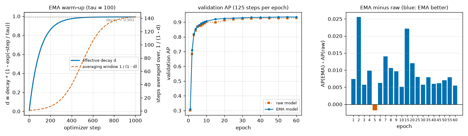
What to read in the left panel of Figure 11-3 is the time lag between the two curves. The blue line (decay) rises early, to 0.86 at 200 steps and 0.986 at 500 steps, while the dotted orange line (averaging length) lags far behind, at 7 and 73 steps at those points. Since the averaging length is \(1/(1 - d_n)\), it only grows once \(d_n\) gets very close to 1. The meaning is this: average over a short window early in training, and over a longer window as training progresses. Early on, the model improves a lot every step, so mixing in old weights hurts; later, the model jitters in one place, so the longer the average, the better.
Appendix A of the paper only says "we use an EMA scheduler as in DINOv3, since it is needed for EMA to work properly." In the public code, the only mechanism that changes the EMA decay over time is this warmup formula.
The weights used for evaluation and saving
The EMA model takes no part in training at all. The forward pass, loss, and backward pass are all done with the regular model, and the EMA model just averages on the side. This differs from DINO in chapter 6, where the output of the EMA-built teacher became the student's target and changed training itself. RF-DETR's EMA is a bystander. So turning EMA on or off has no effect on the training result of the regular model, and a single training run yields both "the result with EMA" and "the result without EMA." The ablations later make use of this property.
It is used after training ends and for scoring during training.
- Evaluation. By default, the official implementation measures validation AP with the EMA weights. Passing
eval_base_model=Truealso scores the regular weights and records them separately. - Saving and deployment. The official implementation keeps the weights from the epoch with the best validation AP for the EMA weights as
checkpoint_best_ema.pth. If the regular weights were also scored, it also keeps their best (checkpoint_best_regular.pth), and the better of the two becomes the final modelcheckpoint_best_total.pth(chapter 14).
Why might averaged weights be better? One explanation is that the regular weights are values jittered to suit the last few batches, while the EMA weights have had that jitter removed. As seen in chapter 6, the DINO paper also reports that the EMA teacher outperformed the student throughout training. But averaging is not always a gain. In phases where the model improves quickly, an average that mixes in the past lags behind the current model. Which one actually scores higher is measured twenty times in this chapter's experiments.
Layer-wise learning rate decay
So far the learning rate has been called "1e-4," but not every weight learns at that rate. RF-DETR uses a different learning rate for each component and, within the backbone, for each block.
A little for shallow layers, more for deep layers
Fine-tuning starts from a pretrained backbone (chapter 6). Not every layer of that backbone needs to be "adjusted for the new task" to the same degree.
- Shallow blocks near the input look at things that apply to any image, such as edges, textures, and colors. They remain useful on new data as they are, and changing them carelessly would overwrite what was learned from hundreds of millions of images with a few thousand.
- Deep blocks near the output produce features tuned to the pretraining objective (self-distillation, for DINOv2). They need more adjustment for the new objective of detection.
- Newly attached components (projector, decoder, heads) have not been trained as long as the backbone, or must learn from scratch. They are adjusted the most.
Turning this idea into numbers gives layer-wise learning rate decay. Starting from the top block of the backbone, the learning rate is multiplied by a number less than 1 (0.8 for RF-DETR) for each block one goes down toward the input. Appendix A of the paper says it "applies a multiplicative decay of 0.8 per layer to preserve the information in the DINOv2 backbone (especially in the early layers)."
- Caution · Three kinds of "decay"
- This chapter has three similarly named things: weight decay (chapter 4: pulling the weights slightly toward 0 at every step), EMA decay \(d\) (how much of the old average to keep), and layer-wise learning rate decay (how much to reduce the learning rate per layer). They are three unrelated numbers. Also, a "deep block" here is a block near the output, and a "shallow block" is one near the input.
The formula in the official code
The paper only gives the number "0.8," so the exact formula is read from the public code (get_dinov2_lr_decay_rate and get_named_param_lr_pairs in models/backbone/backbone.py). In short, it is the following two steps.
The rule the official implementation uses to set backbone parameter learning rates (abridged)
num_layers = out_feature_indexes[-1] + 1            # Nano: [3, 6, 9, 12] → 13
layer_id = num_layers + 1                           # 기본: 맨 위 (감쇠 없음)
if "embeddings" in name:                            # 패치 임베딩 · 위치 임베딩 · CLS 토큰
    layer_id = 0
elif ".layer." in name:                             # 블록 j 의 매개변수
    layer_id = j + 1
lr = lr_encoder * lr_vit_layer_decay ** (num_layers + 1 - layer_id) * lr_component_decay ** 2
In symbols (using the same letters as chapter 14):
- \(\eta\): the base learning rate
lr. \(\eta_{\text{enc}}\): the backbone's base learning ratelr_encoder. - \(\lambda\) (lambda): the layer-wise decay rate
lr_vit_layer_decay= 0.8. \(\rho\) (rho): the per-component decay ratelr_component_decay= 0.7. - \(L\):
num_layersin the code. \(i\): the parameter's layer indexlayer_id. \(j\): the backbone block index (from 0). In the loss sections \(i\) and \(j\) were query and ground-truth indices, but in this section they are layer and block indices.
\(\text{backbone parameter learning rate} \;=\; \eta_{\text{enc}} \cdot \lambda^{\,L + 1 - i} \cdot \rho^{2}, \qquad i = \begin{cases} 0 & \text{embeddings} \\ j + 1 & \text{block } j \ (j = 0, 1, \dots) \\ L + 1 & \text{otherwise (final layer norm)} \end{cases}\)
The exponent \(L + 1 - i\) of \(\lambda\) is "how many steps below the top." Block \(j\) has \(i = j + 1\), so its exponent is \(L - j\).
- Note · How the layer count L is counted
- The public code sets \(L\) not to the number of blocks but to the index of the last feature-extraction point + 1. For Nano, Small, and Medium that index is 12 (the output after all 12 blocks), so \(L = 13\), one more than the number of blocks. As a result, the top block (block 11) gets a multiplier of \(0.8^{13 - 11} = 0.8^2 = 0.64\), not \(0.8^1\). This is the actual behavior of the code, which cannot be inferred from the paper's "0.8 per layer" alone. This tutorial follows the behavior of the public code. The mini model has 6 blocks with extraction points (2, 4, 6), so \(L = 7\).
Multiplier table for twelve blocks
Build the table for RF-DETR Nano (12 backbone blocks, \(L = 13\)) by hand. Powers of \(0.8\) are obtained by multiplying the previous value by 0.8.
- Hand calculation — powers of 0.8 and the common factor
- \(0.8^2 = 0.64, \quad 0.8^3 = 0.512, \quad 0.8^4 = 0.4096, \quad 0.8^5 = 0.32768, \quad 0.8^6 = 0.26214, \quad 0.8^7 = 0.20972\)
- Multiply by 0.8 in turn: \(0.64 \times 0.8 = 0.512\), \(0.512 \times 0.8 = 0.4096\), …
- Keep multiplying. After fourteen multiplications it is 4.4% of the original.
- The factor common to every backbone parameter. It is also the learning rate at "the top," where no layer-wise decay applies.
- The top block. The exponent is \(L - j = 13 - 11 = 2\).
- The bottom block. It is \(0.8^{11} = 0.0859\) times the top block, or about 1/11.6.
| Part | Layer index \(i\) | Exponent \(L + 1 - i\) | Multiplier \(0.8^{\,L + 1 - i}\) | Learning rate (\(7.35 \times 10^{-5}\) × multiplier) | Multiple of the base learning rate \(10^{-4}\) |
| Embeddings (patch, position, CLS) | 0 | 14 | 0.04398 | \(3.23 \times 10^{-6}\) | 0.032 |
| Block 0 | 1 | 13 | 0.05498 | \(4.04 \times 10^{-6}\) | 0.040 |
| Block 1 | 2 | 12 | 0.06872 | \(5.05 \times 10^{-6}\) | 0.051 |
| Block 2 | 3 | 11 | 0.08590 | \(6.31 \times 10^{-6}\) | 0.063 |
| Block 3 | 4 | 10 | 0.10737 | \(7.89 \times 10^{-6}\) | 0.079 |
| Block 4 | 5 | 9 | 0.13422 | \(9.87 \times 10^{-6}\) | 0.099 |
| Block 5 | 6 | 8 | 0.16777 | \(1.23 \times 10^{-5}\) | 0.123 |
| Block 6 | 7 | 7 | 0.20972 | \(1.54 \times 10^{-5}\) | 0.154 |
| Block 7 | 8 | 6 | 0.26214 | \(1.93 \times 10^{-5}\) | 0.193 |
| Block 8 | 9 | 5 | 0.32768 | \(2.41 \times 10^{-5}\) | 0.241 |
| Block 9 | 10 | 4 | 0.40960 | \(3.01 \times 10^{-5}\) | 0.301 |
| Block 10 | 11 | 3 | 0.51200 | \(3.76 \times 10^{-5}\) | 0.376 |
| Block 11 | 12 | 2 | 0.64000 | \(4.70 \times 10^{-5}\) | 0.470 |
| Final layer norm | 14 | 0 | 1 | \(7.35 \times 10^{-5}\) | 0.735 |
What to read from the table: the learning rates of two neighboring blocks always differ by a factor of 0.8, and stacked twelve times, the bottom block learns at 1/11.6 the rate of the top block. The embeddings learn at 3.2% of the heads (base learning rate \(10^{-4}\)), about 1/31. The top row of this table, \(3.23 \times 10^{-6}\), equals the smallest learning rate printed in the actual training log in chapter 14 (lr_min 3.233e-06).
Per-component decay and the backbone learning rate
The \(\rho^2\) in the formula above is not specific to the backbone; it is part of a larger rule. The official implementation splits the model into three parts and multiplies each part's learning rate by \(\rho = 0.7\) zero, one, or two times.
| Part | Learning rate | With official defaults | In the mini experiment (\(\eta = 2 \times 10^{-4}\)) |
| Everything else: projector, two-stage heads, classification and box heads, query embeddings | \(\eta\) | \(1.0 \times 10^{-4}\) | \(2.0 \times 10^{-4}\) |
| Decoder | \(\eta \cdot \rho\) | \(7.0 \times 10^{-5}\) | \(1.4 \times 10^{-4}\) |
| Backbone (top reference) | \(\eta_{\text{enc}} \cdot \rho^2\) | \(7.35 \times 10^{-5}\) | \(1.47 \times 10^{-4}\) |
| Backbone block \(j\) | \(\eta_{\text{enc}} \cdot \rho^2 \cdot \lambda^{\,L - j}\) | \(4.04 \times 10^{-6}\) – \(4.70 \times 10^{-5}\) | \(3.08 \times 10^{-5}\) – \(9.41 \times 10^{-5}\) |
- The backbone's base learning rate \(\eta_{\text{enc}} = 1.5\,\eta\) is larger than the base learning rate. But it is multiplied by \(\rho^2 = 0.49\), so it is effectively \(1.5 \times 0.49 = 0.735\) times, and the layer-wise decay is multiplied on top of that. It has to be read as the product of three numbers.
- Structurally, the projector sits between the backbone and the decoder, but under this rule it falls into "everything else" and learns at the base learning rate. This is the actual behavior of the official code.
- The backbone's weight decay also has exceptions. Biases, layer norms, and embeddings get no weight decay (0). Everything else gets \(10^{-4}\).
Here is the result of applying this rule to the mini model, printed by the lab code before training.
[매개변수 그룹] 기본 학습률 2e-4, lr_encoder 3e-4, 층별 감쇠 0.8, 구성 요소별 감쇠 0.7
    그룹                    | 학습률     | 기본 학습률의 몇 배 | 매개변수 수
    backbone: embeddings    | 2.466e-05 |    0.123          |    32,640
    backbone: block 0       | 3.083e-05 |    0.154          |   112,032
    backbone: block 1       | 3.854e-05 |    0.193          |   112,032
    backbone: block 2       | 4.817e-05 |    0.241          |   112,032
    backbone: block 3       | 6.021e-05 |    0.301          |   112,032
    backbone: block 4       | 7.526e-05 |    0.376          |   112,032
    backbone: block 5       | 9.408e-05 |    0.470          |   112,032
    backbone: final norm    | 1.470e-04 |    0.735          |       192
    projector               | 2.000e-04 |    1.000          |   300,544
    two-stage heads         | 2.000e-04 |    1.000          |   202,780
    decoder                 | 1.400e-04 |    0.700          |   584,096
    class + box heads       | 2.000e-04 |    1.000          |    33,927
    query embeddings        | 2.000e-04 |    1.000          |     6,336
- Figure: Figure 11-4 Learning rate per parameter group of the mini RF-DETR (in units of \(10^{-4}\)). Blue: the official rule (layer-wise decay 0.8, per-component decay 0.7, backbone base learning rate 1.5×). Orange hatched: the same learning rate for every group (used as "constant learning rate" in the ablations later). The numbers in parentheses below the axis labels are the parameter counts of each group.
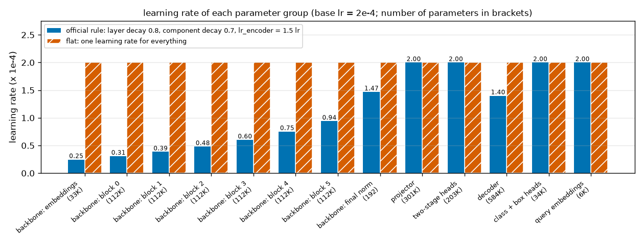
The blue bars in Figure 11-4 form a staircase running from left to right at 0.25, 0.31, 0.39, 0.48, 0.60, 0.75, 0.94. The ratio between neighboring bars is always 0.8. Checking by hand, block 5 is \(3 \times 10^{-4} \times 0.8^{7 - 5} \times 0.49 = 3 \times 10^{-4} \times 0.64 \times 0.49 = 9.408 \times 10^{-5}\) and the embeddings are \(3 \times 10^{-4} \times 0.8^{8} \times 0.49 = 3 \times 10^{-4} \times 0.16777 \times 0.49 = 2.466 \times 10^{-5}\), matching the output. After the staircase come the final layer norm at 1.47, the projector and heads at 2.00, and the decoder at 1.40. The first backbone block learns at 0.154 times the speed of the projector, about 1/6.5. This figure is determined by the rule alone, independent of training.
- Caution · The main experiment in this chapter applies this rule to a random backbone
- Layer-wise learning rate decay is a mechanism for protecting a pretrained backbone. But the main experiment in this chapter initializes the backbone randomly (there is no DINOv2 for the shapes world). It amounts to telling a backbone with nothing to protect to "change only a little," so there is no guarantee this combination is best. It was done this way on the principle of scaling down the official settings as they are, and what that costs is measured in ablation (e) later.
Augmentation and multi-resolution
The third question is "what to show the model." Showing training images not just as they are but transformed, by flipping or cropping, is called data augmentation. It gets the effect of several images out of one and reduces overfitting when data is scarce. In detection with boxes, when the image is transformed the boxes must be transformed in the same way. For example, a horizontal flip changes only the horizontal center coordinate of a normalized box, \(c_x \to 1 - c_x\): \((0.30, 0.40, 0.20, 0.10)\) becomes \((0.70, 0.40, 0.20, 0.10)\).
Only flips and crops
Real-time detectors use augmentation very aggressively. Just the examples given in Section 3 of the paper include vertical flips, random resizing, random cropping, color jitter (YOLOX-style HSV augmentation), and mixing images together (MixUp). The paper makes two points.
- Augmentation is an assumption about the data. It helps only when the assumption "the image is still plausible after this transformation" holds. The paper notes that augmentation presupposes knowing the properties of the dataset in advance, and in that sense introduces the same kind of bias as a learning rate schedule.
- A wrong assumption is harmful. The paper's example is vertical flipping. A person detector for a self-driving car should not be trained on upside-down images, because it could end up detecting a person reflected (upside down) in a puddle as a person.
The shapes world has the same kind of example. Triangles in this world always have their apex at the top. A horizontally flipped image is still an image from the shapes world, but a vertical flip creates a triangle with its apex at the bottom, which does not exist in this world. A detector trained on such images spends capacity learning things that do not exist.
So RF-DETR restricts augmentation to two kinds, horizontal flip and random crop (Section 3 of the paper), keeping only those that are generally safe on any data. There is also no schedule for turning augmentation on and off during training. That is why "scheduler-free" also refers to augmentation.
Resizing per batch
Another augmentation is multi-resolution training (also called multi-scale training). The resolution of the input images is changed randomly during training so that the model gets used to objects that appear both large and small. This is different from the "multi-scale features" of chapter 8 (extracting feature maps at several resolutions from one image); here the size of the input image itself changes.
RF-DETR changes LW-DETR's approach in two places (Section 3 and Appendix A of the paper).
| LW-DETR | RF-DETR | |
| Unit for choosing the size | A random size for each image separately; the rest are padded to match the largest image in the batch | Per batch: one size is chosen per batch and the whole batch is resized to it |
| Size range | 0.7–1.4× the base resolution | 0.5–1.5× (symmetric around the base resolution) |
| Role of resolution | Data augmentation | Augmentation and also a NAS knob (chapter 12) |
Why choosing a size per image is bad becomes clear with numbers. Suppose the four images of a batch are assigned side lengths 448, 512, 640, and 704 (an illustrative example). To pack the four into one tensor, all must be brought to 704 × 704.
\(\frac{448^2 + 512^2 + 640^2 + 704^2}{4 \times 704^2} = \frac{200{,}704 + 262{,}144 + 409{,}600 + 495{,}616}{1{,}982{,}464} = \frac{1{,}368{,}064}{1{,}982{,}464} = 0.69\)
Only 69% of the tensor is actual image and 31% is padding. The paper notes that with this approach most images get large padding, which creates artifacts in window attention (such as a window that is entirely padding) and wastes computation on the padded area. Resizing the whole batch to the same size eliminates padding caused by size differences. The paper also gives as a reason that this makes every positional encoding resolution appear evenly during training. Because the model interpolates its position embeddings to match the resolution (chapter 6), this avoids seeing some resolutions often and others hardly at all.
- Note · Resolution list in the public code
- The official implementation's defaults are
multi_scale="per-batch"andexpanded_scales=True. The resolution list is built by varying "how many patches fit along one side of a window" from −5 to +5 around the default. For Nano (resolution 384, patch 16, 2 windows per side), the default is \(384 / (16 \times 2) = 12\), so there are 11 sizes from \(7 \times 32 = 224\) to \(17 \times 32 = 544\) in steps of 32, which is 0.58–1.42× the base resolution. With resolution 560, patch 14, and 4 windows, the range is \(5 \times 56 = 280\) to \(15 \times 56 = 840\), exactly the paper's 0.5–1.5×. The rule ensures the resolution is always a multiple of patch size × number of windows.
The mini experiment in this chapter uses neither augmentation nor multi-resolution training. The shapes-world images are synthetic data generated randomly, so the 4,000 images are already distinct scenes, and training with varying resolution is the topic of chapter 12. train_one_epoch in the lab code has an option to change resolution per batch (resolutions), but it is turned off in this chapter.
The pretraining ladder
The last question is "where to start." This starting point is exactly what the settings so far, the low learning rate and the layer-wise decay, were meant to protect. RF-DETR's weights go through two rounds of training before they meet the target data.
Original figure 11-5. The three stages RF-DETR's weights go through. The result (weights) of each stage becomes the initial value of the next. Moving right, the data gets smaller and the task gets closer to the target.
- ① Self-supervised pretraining: DINOv2. 142 million unlabeled images. What is trained is the backbone (chapter 6).
- ② Supervised detection pretraining: Objects365. Large detection data with box labels. What is trained is the whole model. Segmentation is trained with pseudo-labels from SAM2.
- ③ Fine-tuning: target data (COCO, RF100-VL, your own data). What is trained is the whole model, and this chapter's training settings apply here.
- DINOv2: self-supervised pretraining. The backbone starts from the weights of DINOv2, trained on 142 million unlabeled images (chapter 6). The paper states that initializing the backbone with DINOv2's pretrained weights greatly improves detection accuracy on small datasets (Section 3).
- Objects365: supervised detection pretraining. A backbone alone is not a detector. The projector, decoder, and heads need box labels to learn. So the whole model is first trained on the large detection dataset Objects365 (chapter 1). This stage is inherited from LW-DETR. Segmentation models need mask labels, but Objects365 has only boxes, so the paper generates masks with SAM2 and attaches them as pseudo-labels, pretraining the detection head and the segmentation head on the same data (Appendix A, chapter 13).
- Target data: fine-tuning. Starting from the weights built this way, the model is trained on the target data. The weights the
rfdetrpackage downloads have completed up to ②, and what the user does is ③ (chapter 14).
How much each stage contributes is shown in tables from the two papers. All values are measured on COCO.
| Source | Comparison | COCO AP |
| RF-DETR paper, Table 5 | LW-DETR (M) | 52.6 |
| + gentler hyperparameters (lower learning rate, batch norm → layer norm, etc.) | 51.6 | |
| + DINOv2 backbone | 53.6 | |
| + Objects365 pretraining added | 54.3 | |
| RF-DETR paper, Table 6 | CAEv2 ViT-S/16 backbone (LW-DETR's backbone) | 52.3 |
| DINOv2 ViT-S/14 backbone | 54.3 | |
| SigLIPv2 ViT-B/32 backbone | 50.4 | |
| SAM2 Hiera-S backbone | 53.6 | |
| LW-DETR paper, Table 5 | LW-DETR small: without → with Objects365 pretraining | 43.6 → 48.0 |
| LW-DETR medium: without → with | 47.2 → 52.5 |
- The second row of Table 5 is worth noting. Switching to gentler training settings by itself lowers the COCO score by 1.0. The paper does not hide this loss; it states that replacing batch norm with layer norm costs performance but is necessary for training on consumer hardware. The paper's explanation is that the DINOv2 backbone (+2.0) makes up for that loss, and that the low learning rate helps preserve DINOv2's knowledge. The settings and the backbone form a package that cannot be evaluated separately.
- Table 6 compares only the backbone under the same settings (every model in the table was pretrained on Objects365 for 60 epochs). DINOv2 is 2.0 higher than CAEv2.
- Table 5 of the LW-DETR paper compares with and without Objects365 pretraining: +4.4 for small and +5.3 for medium. In Table 2 of the same paper (12-epoch setting), it was +8.7.
All these figures come from photographic data (COCO) and real pretrained weights. Whether the mini experiment in the shapes world shows the same effect has to be checked separately, and to give the conclusion up front, it did not show up in this chapter's mini experiment. This is examined in detail in ablation (e) later.
Walking through the implementation
Now read code/ch11_train.py. The model is MiniRFDETR from chapter 10 as is, and this file contains only what is needed to train it: the loss (RFDETRCriterion), EMA (ModelEMA), parameter groups and the optimizer (build_optimizer), and the training loop. IA-BCE and per-group matching come from chapter 9's ch09_lwdetr_parts.py, box operations from chapter 2, and scoring from chapter 3's file.
Running it
There are three run modes, run one at a time.
Terminal
$ python ch11_train.py                # 본 실험: 60 에폭 학습 + 분석 (약 17분)
$ python ch11_train.py --ablations    # 절제 (a) – (d): 15 에폭짜리 학습 네 번 (약 16분). --seed 1 처럼 시드를 바꿀 수 있다
$ python ch11_train.py --pretrain     # 절제 (e): 백본 사전 학습과 비교 (약 25분)
$ python ch11_train.py --quick        # 연기 시험 (CPU 약 20초). --quick --ablations, --quick --pretrain 도 된다
The times were measured on a single 8 GB laptop GPU, but with several runs going at the same time, so a run on its own is faster. The model is small, so one step takes about 0.1 seconds, and most of that is not GPU computation but round trips between Python and the Hungarian solver. The main experiment saves ch11_rfdetr.pt (regular weights, EMA weights, and model config) and ch11_history.json in the run folder. Chapters 12 and 13 start from this checkpoint. If the chapter 7 and chapter 8 experiments were run first (ch07_history.json, ch08_history.json, ch08_deformable.pt), their curves are plotted alongside.
Loss: RFDETRCriterion
ch11_train.py · criterion
class RFDETRCriterion(nn.Module):
    """RF-DETR 의 집합 손실 (공식 criterion.py 의 SetCriterion 과 같은 식).

    층 하나(마지막 디코더 층, 앞 디코더 층들, 인코더 제안)마다
      1) 질의 묶음마다 따로 헝가리안 매칭.  비용 = 2·C_cls(포컬 꼴) + 5·C_L1 + 2·C_GIoU
      2) 분류: IA-BCE (cls_loss="ia_bce", 9장) 또는 포컬 손실 (cls_loss="focal", 8장 — 절제 실험용)
      3) 박스: 매칭된 쌍의 L1 합, (1 − GIoU) 합
      세 손실 모두 num_boxes = (배치의 정답 수) × (묶음 수) 로 나눈다.
    전체 = Σ_층 (1·loss_ce + 5·loss_bbox + 2·loss_giou).
    학습 모드(self.training)에서는 묶음 group_detr 개, 평가 모드에서는 1개로 본다 (모델의 출력과 맞춘다).
    """

    def __init__(self, num_classes: int = NUM_CLASSES, group_detr: int = 4, cls_loss: str = "ia_bce",
                 loss_ce: float = 1.0, loss_bbox: float = 5.0, loss_giou: float = 2.0,
                 alpha: float = 0.25, gamma: float = 2.0):
        super().__init__()
        assert cls_loss in ("ia_bce", "focal")
        self.num_classes, self.group_detr, self.cls_loss = num_classes, group_detr, cls_loss
        self.alpha, self.gamma = alpha, gamma
        self.matcher = GroupHungarianMatcher(cost_class=2.0, cost_bbox=5.0, cost_giou=2.0)
        self.weights = {"loss_ce": loss_ce, "loss_bbox": loss_bbox, "loss_giou": loss_giou}

    @torch.no_grad()
    def match_layers(self, layers, targets, groups: int):
        """여러 층의 매칭을 한꺼번에 한다 (비용 행렬을 GPU 에서 한 번에 만들고 CPU 로 한 번만 옮긴다).

        layers: [{"pred_logits": (B, Q, K), "pred_boxes": (B, Q, 4)}, …]  (Q = 묶음 수 × N)
        돌려주는 값: 층마다 (batch_idx, query_idx, tgt_idx) — 각각 (M,) LongTensor (M = 정답 수 × 묶음 수).
          k 번째 짝: 예측 pred[batch_idx[k], query_idx[k]] ↔ 배치의 정답을 한 줄로 이어 붙인 것의 tgt_idx[k] 번째.
        """
        logits = torch.stack([layer["pred_logits"] for layer in layers])  # (S, B, Q, K)
        boxes = torch.stack([layer["pred_boxes"] for layer in layers])  # (S, B, Q, 4)
        num_layers, batch, total = logits.shape[:3]
        sizes = [len(t["labels"]) for t in targets]
        offsets = np.cumsum([0] + sizes)
        cost = self.matcher.cost_matrix(logits.flatten(0, 2), boxes.flatten(0, 2),
                                        torch.cat([t["labels"] for t in targets]),
                                        torch.cat([t["boxes"] for t in targets]))
        cost = cost.view(num_layers, batch, total, -1).cpu().numpy()  # (S, B, Q, ΣT)
        layer_ids, batch_ids, query_ids, target_ids = [], [], [], []
        for s in range(num_layers):
            for b in range(batch):
                if sizes[b] == 0:
                    continue
                rows, cols = self.matcher.assign_groups(cost[s, b, :, offsets[b]:offsets[b + 1]], groups)
                layer_ids.append(np.full(len(rows), s))
                batch_ids.append(np.full(len(rows), b))
                query_ids.append(rows)
                target_ids.append(cols + offsets[b])
        index = np.stack([np.concatenate(ids) for ids in (layer_ids, batch_ids, query_ids, target_ids)])
        index = torch.as_tensor(index, dtype=torch.long, device=logits.device)  # (4, 전체 짝 수): 한 번에 장치로
        return [tuple(index[1:, index[0] == s]) for s in range(num_layers)]

    def layer_loss(self, layer, matched, tgt_labels, tgt_boxes, num_boxes):
        """층 하나의 세 손실. tgt_labels (ΣT,), tgt_boxes (ΣT, 4): 배치의 정답을 이어 붙인 것."""
        batch_idx, query_idx, tgt_idx = matched
        pred = layer["pred_boxes"][batch_idx, query_idx]  # (M, 4)
        target = tgt_boxes[tgt_idx]  # (M, 4)
        pred_xyxy, target_xyxy = box_cxcywh_to_xyxy(pred), box_cxcywh_to_xyxy(target)
        loss_bbox = F.l1_loss(pred, target, reduction="sum") / num_boxes
        loss_giou = (1 - paired_generalized_box_iou(pred_xyxy, target_xyxy)).sum() / num_boxes
        logits = layer["pred_logits"]
        if self.cls_loss == "ia_bce":
            ious = paired_box_iou(pred_xyxy.detach(), target_xyxy)  # 지금 이 예측 박스가 정답과 얼마나 겹치는가
            loss_ce = ia_bce_loss(logits, (batch_idx, query_idx), tgt_labels[tgt_idx], ious, num_boxes,
                                  self.alpha, self.gamma)
        else:
            onehot = torch.zeros_like(logits)
            onehot[batch_idx, query_idx, tgt_labels[tgt_idx]] = 1.0
            loss_ce = sigmoid_focal_loss(logits, onehot, self.alpha, self.gamma).sum() / num_boxes
        return {"loss_ce": loss_ce, "loss_bbox": loss_bbox, "loss_giou": loss_giou}

    def forward(self, outputs, targets, return_matches: bool = False):
        """outputs: MiniRFDETR 의 출력 사전, targets: 길이 B 의 목록 ({"labels": (T_b,), "boxes": (T_b, 4)}).

        돌려주는 값: 손실 사전. "loss" 가 역전파할 전체 손실. "loss_ce" · "loss_bbox" · "loss_giou" 는 마지막 디코더 층,
        "loss_ce_0" … 은 앞 층들, "loss_ce_enc" … 은 인코더 제안의 값 (계수를 곱하기 전).
        return_matches=True 면 (손실 사전, 매칭 목록) — 매칭 목록의 순서는 [마지막 층, 앞 층 0, 앞 층 1, …, 인코더 제안].
        """
        groups = self.group_detr if self.training else 1
        layers = [outputs] + list(outputs.get("aux_outputs", []))
        suffixes = [""] + [f"_{i}" for i in range(len(layers) - 1)]
        if "enc_outputs" in outputs:
            layers.append(outputs["enc_outputs"])
            suffixes.append("_enc")
        tgt_labels = torch.cat([t["labels"] for t in targets])
        tgt_boxes = torch.cat([t["boxes"] for t in targets])
        num_boxes = max(len(tgt_labels) * groups, 1)
        matches = self.match_layers(layers, targets, groups)
        losses = {}
        for layer, suffix, matched in zip(layers, suffixes, matches):
            for name, value in self.layer_loss(layer, matched, tgt_labels, tgt_boxes, num_boxes).items():
                losses[name + suffix] = value
        losses["loss"] = sum(self.weights["_".join(k.split("_")[:2])] * v for k, v in losses.items())
        return (losses, matches) if return_matches else losses
-
forwardis exactly the formula seen earlier. It builds the list of siteslayersin the order [last layer, earlier layers, encoder proposals] (suffixes"","_0","_1","_enc"), computesnum_boxes = number of ground truths × number of groups, and callslayer_lossfor each site to put the three losses into the dictionary. The last line is the weighted sum with coefficients 1, 5, and 2. Since the coefficient is looked up by the first two segments of the name (loss_ce, etc.), the same coefficient is used even with a suffix attached. -
groups = self.group_detr if self.training else 1: there are multiple groups only during training. In evaluation mode the model outputs only the first group's queries, so the loss must be put in the same mode. That is why the training loop callsmodel.train()andcriterion.train()together. -
match_layersis batching for speed. It stacks the logits(S, B, Q, K)and boxes(S, B, Q, 4)of the four sites (\(S\) is the number of sites, \(Q = G \cdot N\)), builds the cost matrix(S, B, Q, ΣT)on the GPU in one go, and moves it to the CPU only once. Then, for each site and each image, chapter 9'sassign_groupsruns the Hungarian solver per group. What it returns is, for each site, three index vectors (image index, query index, ground-truth index), all with length equal to the number of matches (number of ground truths × number of groups,Min the code comments). The whole function is under@torch.no_grad(); matching has no gradient. - In
layer_loss,pred = layer["pred_boxes"][batch_idx, query_idx]picks the matched predicted boxes(M, 4), andtgt_boxes[tgt_idx]picks their ground-truth boxes(M, 4). L1 takes the sum and GIoU takes the sum of \(1 - \operatorname{GIoU}\), each divided bynum_boxes. - The IoU passed to IA-BCE is computed with
pred_xyxy.detach(). No gradient flows to the boxes through the IoU used to build the target; boxes learn only through the box losses. -
cls_loss="focal"is for the ablations. It puts chapter 8's focal loss in place of IA-BCE but keeps the coefficient at 1. This corresponds to turning off only theia_bce_losssetting in the official implementation (it differs from chapter 8's Deformable DETR experiment, which used a coefficient of 2).
EMA: ModelEMA
ch11_train.py · ema
class ModelEMA:
    """가중치의 지수 이동 평균. 공식 구현(RFDETREMACallback)과 같은 식이다.

    옵티마이저가 한 스텝 갈 때마다:   θ_ema ← d·θ_ema + (1 − d)·θ
    감쇠 d 는 처음에 0 에서 출발해 decay 로 올라간다:   d = decay · (1 − exp(−스텝 수 / τ))   (decay 0.993, τ 100)
    처음 몇 스텝은 d ≈ 0 이라 EMA 가 모델을 그대로 따라가므로, 무작위 초기값이 평균에 오래 남지 않는다.
    평가 · 배포에는 self.module (EMA 가중치를 가진 모델 사본) 을 쓴다.
    """

    def __init__(self, model: nn.Module, decay: float = 0.993, tau: float = 100.0):
        self.module = copy.deepcopy(model).eval()
        for p in self.module.parameters():
            p.requires_grad_(False)
        self.decay, self.tau, self.updates = decay, tau, 0

    def effective_decay(self, updates: int) -> float:
        return self.decay * (1 - math.exp(-updates / self.tau)) if self.tau > 0 else self.decay

    @torch.no_grad()
    def update(self, model: nn.Module):
        self.updates += 1
        d = self.effective_decay(self.updates)
        for ema_p, p in zip(self.module.parameters(), model.parameters()):
            ema_p.lerp_(p, 1 - d)  # ema + (1 − d)·(θ − ema) = d·ema + (1 − d)·θ
-
copy.deepcopy(model)makes the copy and turns off gradient computation for it. The copy is always in evaluation mode. One more model sits in memory. -
effective_decayis the warmup formula \(d_n = d\,(1 - e^{-n/\tau})\). Each call toupdatefirst incrementsself.updatesby 1, so \(n\) counts from 1, the same counting as in the official implementation. -
ema_p.lerp_(p, 1 - d)is an in-place operation meaning "move fromema_ptowardpby \((1 - d)\)." Expanded, it is \(\theta_{\text{ema}} + (1 - d)(\theta - \theta_{\text{ema}}) = d\,\theta_{\text{ema}} + (1 - d)\,\theta\), the same as the update rule. - The official implementation averages not only the weights but also the buffers (non-trainable state such as batch normalization statistics), but this mini model has no buffers, so only the weights are averaged.
Parameter groups and the optimizer
ch11_train.py · param-groups
def vit_layer_id(name: str, num_layers: int) -> int:
    """백본 매개변수의 "층 번호": 임베딩(패치 · CLS · 위치) 0, 블록 i 는 i + 1, 그 밖(마지막 층 정규화)은 num_layers + 1.

    공식 get_dinov2_lr_decay_rate 와 같은 규칙. 학습률 배율은 decay ** (num_layers + 1 − 층 번호) 이다.
    """
    if name.startswith("backbone.blocks."):
        return int(name.split(".")[2]) + 1
    if name.startswith(("backbone.patch_embed", "backbone.cls_token", "backbone.mask_token", "backbone.pos_embed")):
        return 0
    return num_layers + 1


def build_param_groups(model: MiniRFDETR, lr: float = 2e-4, lr_encoder: float | None = None,
                       vit_layer_decay: float = 0.8, component_decay: float = 0.7, weight_decay: float = 1e-4):
    """공식 param_groups.py 의 규칙으로 매개변수마다 학습률 · 가중치 감쇠를 정한다.

      백본(ViT)        lr_encoder · vit_layer_decay^(num_layers + 1 − 층 번호) · component_decay²
                       num_layers = out_feature_indexes[-1] + 1 (공식 구현이 이렇게 센다 — 블록 수보다 1 크다).
                       편향 · 층 정규화 · 임베딩(패치 임베딩의 가중치 포함)은 가중치 감쇠 0
      디코더           lr · component_decay        (디코더 층, decoder_norm, ref_point_head)
      그 밖            lr                          (프로젝터, 2단계 머리, 분류 · 박스 머리, 질의 임베딩)
    lr_encoder 를 주지 않으면 공식 기본값의 비율(1.5e-4 / 1e-4)대로 1.5 · lr.
    돌려주는 값: (옵티마이저에 넘길 그룹 목록, 사람이 읽을 표 [(이름, 학습률, 가중치 감쇠, 매개변수 수)]).
    """
    lr_encoder = 1.5 * lr if lr_encoder is None else lr_encoder
    num_layers = model.config["out_feature_indexes"][-1] + 1
    buckets, table = {}, {}
    for name, p in model.named_parameters():
        if name.startswith("backbone."):
            layer_id = vit_layer_id(name, num_layers)
            p_lr = lr_encoder * vit_layer_decay ** (num_layers + 1 - layer_id) * component_decay**2
            no_decay = layer_id == 0 or name.endswith(".bias") or "norm" in name
            p_wd = 0.0 if no_decay else weight_decay
            label = ("backbone: embeddings" if layer_id == 0 else
                     f"backbone: block {layer_id - 1}" if layer_id <= num_layers else "backbone: final norm")
        elif name.startswith(("decoder.", "decoder_norm.", "ref_point_head.")):
            p_lr, p_wd, label = lr * component_decay, weight_decay, "decoder"
        else:
            p_lr, p_wd = lr, weight_decay
            label = ("projector" if name.startswith("projector.") else
                     "two-stage heads" if name.startswith("enc_") else
                     "query embeddings" if name.startswith(("query_feat", "refpoint_embed")) else "class + box heads")
        buckets.setdefault((p_lr, p_wd), []).append(p)  # 설정이 같은 매개변수는 한 그룹으로
        row = table.setdefault(label, [p_lr, 0])
        row[1] += p.numel()
    groups = [{"params": params, "lr": g_lr, "weight_decay": g_wd} for (g_lr, g_wd), params in buckets.items()]
    return groups, [(label, row[0], row[1]) for label, row in table.items()]


def build_optimizer(model: MiniRFDETR, lr: float = 2e-4, **kwargs):
    """AdamW. 스케줄러는 없다 — RF-DETR 은 학습 내내 같은 학습률을 쓴다 (워밍업도 없다)."""
    groups, table = build_param_groups(model, lr, **kwargs)
    return torch.optim.AdamW(groups, lr=lr, weight_decay=kwargs.get("weight_decay", 1e-4)), table
-
vit_layer_iddetermines the layer index \(i\). If the name starts withbackbone.blocks.j.it is \(j + 1\); for embedding-type parameters (patch embedding, CLS token, mask token, position embedding) it is 0; otherwise (final layer norm) it is \(L + 1\). -
build_param_groupsscans every parameter by name and sets its learning rate and weight decay: \(\eta_{\text{enc}} \cdot \lambda^{L + 1 - i} \cdot \rho^2\) for the backbone, \(\eta \cdot \rho\) for the decoder (decoder layers, the decoder's layer norm, and the reference point head), and \(\eta\) for the rest.num_layers = out_feature_indexes[-1] + 1is the "how \(L\) is counted" seen earlier. - PyTorch optimizers take parameters in groups, and each group can have its own learning rate and weight decay.
bucketsputs parameters with the same (learning rate, weight decay) into one group. This model ends up with a dozen or so groups. -
build_optimizerjust buildsAdamWfrom those groups. There is no line that creates a scheduler. This is the implementation of "scheduler-free training." - The "constant learning rate" setting is obtained by passing
lr_encoder=lr, vit_layer_decay=1.0, component_decay=1.0. Every parameter then gets the same learning rate.
Training loop
ch11_train.py · train-loop — This long code is collapsed in the original and is not reproduced here. It is in the train-loop region of code/ch11_train.py.
One step of train_one_epoch is six lines.
-
criterion(model(images, **kwargs), targets): forward pass and loss. -
optimizer.zero_grad(): clear the previous step's gradients. They are cleared every step, so there is no gradient accumulation. -
losses["loss"].backward(): backpropagate the single total loss. -
clip_grad_norm_(model.parameters(), max_norm): clip the total norm to 0.1. This must come between backpropagation and the update. -
optimizer.step(): the AdamW update. -
ema.update(model): update the EMA once with the updated weights. It must come after the update so that the just-updated weights enter the average.
Compared with the training loop of chapter 7, only the sixth line is new. resolutions and forward_kwargs_fn are placeholders for chapter 12 (weight-sharing NAS, which changes the resolution per batch and the architecture per step). They are not used in this chapter.
fit records the loss every epoch, and on scoring epochs (every epoch for the first 10, then every 5) scores both the regular model and the EMA model on the validation set. "AP" in the history is the EMA model's value and "AP_raw" is the regular model's. predict and evaluate_model are inference and scoring functions built to accept forward arguments such as the number of decoder layers, number of queries, and number of windows.
A function wrapping one experiment
ch11_train.py · run — This long code is collapsed in the original and is not reproduced here. It is in the run region of code/ch11_train.py.
run_experiment fixes the seed, builds the model, loss, optimizer, EMA, and data loaders, and calls fit. The main experiment and all the ablations call this one function with different arguments. The ablation knobs are cls_loss (classification loss), vit_layer_decay, component_decay, and lr_encoder (learning rate rule), backbone_state (pretrained backbone), and **model_config (model settings such as the number of groups and windows).
ch11_train.py · main — This long code is collapsed in the original and is not reproduced here. It is in the main region of code/ch11_train.py.
Similarities and differences with the official implementation
| Item | This chapter's lab | Official implementation (defaults) |
| Matching | Same: Hungarian per site and per group, cost 2 · focal form + 5 · L1 + 2 · (−GIoU) | |
| Losses and coefficients | Same: IA-BCE 1, L1 5, GIoU 2. All decoder layers and the encoder proposals. Divided by number of ground truths × number of groups | |
| Optimizer | Same: AdamW, weight decay 1e-4, gradient clipping 0.1, no scheduler or warmup | |
| Learning rate rule | Same: backbone base learning rate 1.5×, layer-wise decay 0.8, per-component decay 0.7, weight decay 0 for backbone biases, layer norms, and embeddings | |
| EMA | Same: decay 0.993, \(\tau\) = 100, updated every step | |
| Base learning rate | 2e-4 | 1e-4 |
| Groups × queries | 4 × 12 | 13 × 300 |
| Batch and epochs | 32, 60 epochs | 4 (gradient accumulation optional), 100 epochs |
| Augmentation and multi-resolution | None | Horizontal flip and random crop, per-batch multi-resolution |
| Backbone initialization | Random (pretrained only in ablation (e)) | DINOv2 → Objects365 pretrained weights |
| Saved weights | Regular and EMA weights from the last epoch | Weights from the epoch with the best validation AP |
| Mixed precision (AMP) | Not used | Used |
The biggest difference is the backbone initialization. The official settings' low learning rate and layer-wise decay presuppose a pretrained backbone, but this chapter's main experiment applies those settings to a random backbone. While building the lab code, the per-group matching assignments and the EMA's effective decay were checked separately against the official implementation's functions and confirmed to be the same (this is not part of this chapter's output).
Reading the results: the main experiment
The model was trained for 60 epochs (7,500 steps) on 4,000 shapes-world training images and scored on 500 validation images (1,265 ground-truth objects). The data, number of epochs, and batch size are the same as in the chapter 7 and chapter 8 experiments. There is one seed (0). The output of the pre-training checks (loss verification, EMA decay, parameter groups) was already shown above.
Training log
[미니 RF-DETR (본 실험)] 매개변수 1,832,707개, 에폭 60, 에폭당 125 스텝, 학습 그림 4000장
에폭   1 | 손실 12.6887 (ce 0.7255 bbox 0.2475 giou 0.5632) | EMA AP 0.3085 AP50 0.6125 AP75 0.2667 | 일반 AP 0.3011 AP50 0.6071 AP75 0.2574 |    20초
에폭   2 | 손실  6.5819 (ce 0.7249 bbox 0.0720 giou 0.2068) | EMA AP 0.7094 AP50 0.9182 AP75 0.8495 | 일반 AP 0.6839 AP50 0.9100 AP75 0.8218 |    40초
에폭   3 | 손실  4.2412 (ce 0.5508 bbox 0.0378 giou 0.1139) | EMA AP 0.8190 AP50 0.9545 AP75 0.9201 | 일반 AP 0.8133 AP50 0.9530 AP75 0.9191 |    60초
에폭   4 | 손실  3.5206 (ce 0.4545 bbox 0.0306 giou 0.0936) | EMA AP 0.8541 AP50 0.9684 AP75 0.9407 | 일반 AP 0.8443 AP50 0.9717 AP75 0.9458 |    80초
에폭   5 | 손실  3.0661 (ce 0.3808 bbox 0.0269 giou 0.0829) | EMA AP 0.8692 AP50 0.9751 AP75 0.9520 | 일반 AP 0.8710 AP50 0.9777 AP75 0.9585 |   101초
에폭   6 | 손실  2.7935 (ce 0.3425 bbox 0.0243 giou 0.0759) | EMA AP 0.8795 AP50 0.9798 AP75 0.9567 | 일반 AP 0.8732 AP50 0.9794 AP75 0.9577 |   122초
에폭   7 | 손실  2.5498 (ce 0.3062 bbox 0.0224 giou 0.0703) | EMA AP 0.8907 AP50 0.9813 AP75 0.9620 | 일반 AP 0.8766 AP50 0.9828 AP75 0.9609 |   139초
에폭   8 | 손실  2.3972 (ce 0.2829 bbox 0.0212 giou 0.0669) | EMA AP 0.8957 AP50 0.9821 AP75 0.9646 | 일반 AP 0.8850 AP50 0.9827 AP75 0.9642 |   159초
에폭   9 | 손실  2.2488 (ce 0.2618 bbox 0.0198 giou 0.0630) | EMA AP 0.9025 AP50 0.9842 AP75 0.9680 | 일반 AP 0.8929 AP50 0.9870 AP75 0.9641 |   179초
에폭  10 | 손실  2.1134 (ce 0.2428 bbox 0.0186 giou 0.0595) | EMA AP 0.9074 AP50 0.9870 AP75 0.9664 | 일반 AP 0.9023 AP50 0.9867 AP75 0.9684 |   198초
에폭  15 | 손실  1.7616 (ce 0.2025 bbox 0.0152 giou 0.0498) | EMA AP 0.9198 AP50 0.9887 AP75 0.9677 | 일반 AP 0.8976 AP50 0.9859 AP75 0.9637 |   278초
에폭  20 | 손실  1.5361 (ce 0.1800 bbox 0.0132 giou 0.0442) | EMA AP 0.9255 AP50 0.9892 AP75 0.9683 | 일반 AP 0.9135 AP50 0.9881 AP75 0.9700 |   356초
에폭  25 | 손실  1.3999 (ce 0.1683 bbox 0.0117 giou 0.0395) | EMA AP 0.9268 AP50 0.9886 AP75 0.9690 | 일반 AP 0.9188 AP50 0.9888 AP75 0.9707 |   427초
에폭  30 | 손실  1.3104 (ce 0.1601 bbox 0.0108 giou 0.0369) | EMA AP 0.9294 AP50 0.9892 AP75 0.9735 | 일반 AP 0.9237 AP50 0.9882 AP75 0.9689 |   506초
에폭  35 | 손실  1.2336 (ce 0.1487 bbox 0.0101 giou 0.0346) | EMA AP 0.9322 AP50 0.9895 AP75 0.9758 | 일반 AP 0.9243 AP50 0.9878 AP75 0.9741 |   577초
에폭  40 | 손실  1.1636 (ce 0.1425 bbox 0.0094 giou 0.0324) | EMA AP 0.9325 AP50 0.9893 AP75 0.9721 | 일반 AP 0.9265 AP50 0.9891 AP75 0.9734 |   654초
에폭  45 | 손실  1.1055 (ce 0.1366 bbox 0.0090 giou 0.0311) | EMA AP 0.9333 AP50 0.9896 AP75 0.9745 | 일반 AP 0.9272 AP50 0.9894 AP75 0.9734 |   730초
에폭  50 | 손실  1.0826 (ce 0.1327 bbox 0.0086 giou 0.0298) | EMA AP 0.9347 AP50 0.9913 AP75 0.9757 | 일반 AP 0.9277 AP50 0.9893 AP75 0.9790 |   806초
에폭  55 | 손실  1.0303 (ce 0.1287 bbox 0.0082 giou 0.0285) | EMA AP 0.9352 AP50 0.9912 AP75 0.9752 | 일반 AP 0.9272 AP50 0.9898 AP75 0.9791 |   888초
에폭  60 | 손실  0.9761 (ce 0.1206 bbox 0.0076 giou 0.0265) | EMA AP 0.9347 AP50 0.9897 AP75 0.9762 | 일반 AP 0.9292 AP50 0.9869 AP75 0.9783 |   964초
학습 끝: 964초
[본 실험] 학습 958초 (7500 스텝), EMA 모델 AP 0.9347 AP50 0.9897 AP75 0.9762 | 일반 모델 AP 0.9292 AP50 0.9869 AP75 0.9783
- Each line shows, from left to right, the total loss, the three losses of the last decoder layer in parentheses (before coefficients), the EMA model's validation AP, the regular model's validation AP, and the cumulative time.
- The "loss" is the sum over the four sites. Computing only the last layer in the last epoch gives \(0.1206 + 5 \times 0.0076 + 2 \times 0.0265 = 0.2116\), and the total 0.9761 is 4.6 times that. It is more than 4 times because the losses of the encoder proposals and earlier layers are each a little larger than the last layer's.
- The classification loss barely decreases during the first two epochs (0.7255 → 0.7249). Meanwhile the box loss drops to a third (L1 0.2475 → 0.0720) and AP rises from 0.31 to 0.71. Training has not stalled. This can be read as follows: IA-BCE's target \(t\) is tied to the IoU of the predicted box, so as the boxes improve the target rises, and the loss saying "raise the score more" grows with it. This is also why this loss was actually small, 0.12, in the pre-training check: at that point the boxes barely overlapped the ground truth, so the target was near 0. The same pattern appears in the actual RF-DETR training log in chapter 14.
- AP reaches 0.82 after just 3 epochs and 0.91 at 10 epochs, then rises slowly and levels off around 0.935.
Training curves
- Figure: Figure 11-6 Training curves of the mini RF-DETR. Left: the three training loss terms of the last decoder layer (after coefficients, log-scale vertical axis). Solid blue: classification (IA-BCE); dotted orange: 5 × L1; dash-dot green: 2 × (1 − GIoU). Right: validation AP50 (blue), AP (orange, thick line), and AP75 (green). Solid lines are the EMA model, dotted lines the regular model.
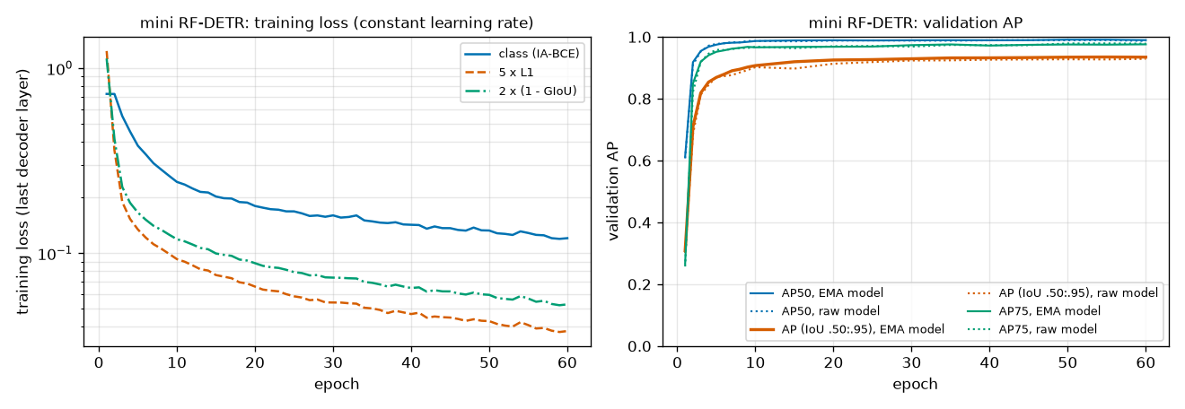
- Left: there are no steps. The loss curves in chapters 7 and 8 had a kink at epoch 48 where the learning rate was lowered. Here the learning rate stays the same to the end, so the three curves descend smoothly. They are still descending at epoch 60.
- The three losses sit at different heights. The two box losses dropped more than tenfold, while the classification loss (blue) descends slowly around 0.12. As seen in the note box earlier, IA-BCE has a floor above 0. With \(t = 0.975\) that floor is \(0.975 \times 0.02532 + 0.025 \times 3.68888 = 0.0247 + 0.0922 = 0.117\), so 0.12 is consistent with the targets of the matches in the training images being roughly that high.
- Right: the loss keeps falling, but validation AP levels off from about epoch 40 (EMA model 0.9325–0.9352). Validation AP does not go down, so there is no sign of overfitting. It is more accurate to say that the model has gotten as much as it can from this model and data.
- The dotted lines (regular model) follow just below the solid lines (EMA model). On the thick orange line, the gap is widest around epoch 15. This is examined separately below.
Overlaid with chapters 7 and 8
- Figure: Figure 11-7 Validation AP (left) and AP75 (right) of three models trained on the same data, for the same number of epochs, with the same batch size. Solid blue: chapter 7 MiniDETR. Dotted orange: chapter 8 Deformable DETR. Dash-dot green: this chapter's mini RF-DETR (EMA model). Dotted pink: the regular weights of the same model. Dots mark scored epochs.
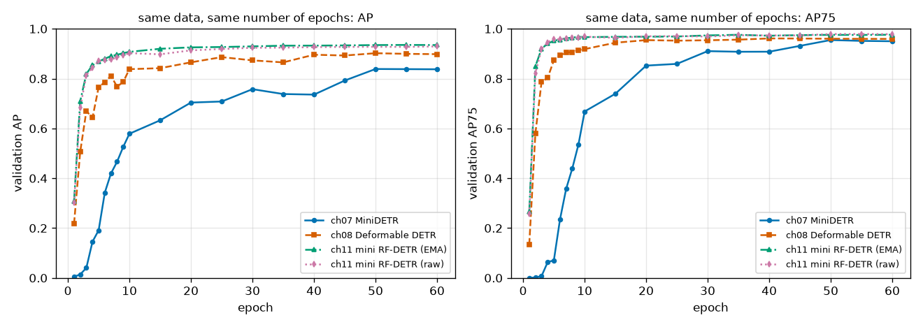
| Epoch | Ch. 7 MiniDETR | Ch. 8 Deformable DETR | Ch. 11 mini RF-DETR (EMA) | Ch. 11 mini RF-DETR (regular) |
| 1 | 0.0048 | 0.2173 | 0.3085 | 0.3011 |
| 3 | 0.0405 | 0.6698 | 0.8190 | 0.8133 |
| 7 | 0.4193 | 0.8109 | 0.8907 | 0.8766 |
| 10 | 0.5788 | 0.8380 | 0.9074 | 0.9023 |
| 20 | 0.7039 | 0.8654 | 0.9255 | 0.9135 |
| 40 | 0.7358 | 0.8959 | 0.9325 | 0.9265 |
| 50 | 0.8386 | 0.9020 | 0.9347 | 0.9277 |
| 60 | 0.8375 | 0.8982 | 0.9347 | 0.9292 |
  ch07 MiniDETR: AP 0.5 / 0.8 / 0.9 에 처음 닿은 에폭 = 9 / 50 / None, 마지막 AP 0.8375
  ch08 Deformable DETR: AP 0.5 / 0.8 / 0.9 에 처음 닿은 에폭 = 2 / 7 / 50, 마지막 AP 0.8982
  ch11 mini RF-DETR (EMA): AP 0.5 / 0.8 / 0.9 에 처음 닿은 에폭 = 2 / 3 / 9, 마지막 AP 0.9347
  ch11 mini RF-DETR (raw): AP 0.5 / 0.8 / 0.9 에 처음 닿은 에폭 = 2 / 3 / 10, 마지막 AP 0.9292
There are two things to read from Figure 11-7. It rises fast: the first epoch to reach AP 0.8 is 50 for chapter 7, 7 for chapter 8, and 3 for this chapter. It goes high: the final APs are 0.8375, 0.8982, and 0.9347. Also, chapter 7's blue line jumps once when the learning rate is lowered at epoch 48 (0.79 → 0.84), whereas the green line has no such intervention and does not seem to need one.
- Caution · This difference cannot be credited to any single component
It is tempting to write "RF-DETR's architecture is better, so 0.90 became 0.93," but this comparison does not say that. Too many things changed between chapter 8's main model and this chapter's model.
- Backbone: a ViT (windowed + global attention) and a C2f projector instead of a small CNN; also one feature level instead of two
- Two-stage query selection (chapter 8's main model did not use it)
- Boxes: box reparameterization and lite reference point refinement (all layers use the same reference boxes) instead of iterative box refinement that updates the reference at each layer
- Classification loss: focal → IA-BCE
- 4 query groups
- EMA
- Learning rate: lowered after epoch 48 → constant to the end, with layer-wise decay
The effect of any one change cannot be read from a comparison that changes seven at once. Instead, two things stand out. In chapter 8's ablations, Deformable DETR with only two-stage added reached AP 0.9100 at 15 epochs. This chapter's model at 15 epochs is 0.9198 for the EMA model and 0.8976 for the regular model (the chapter 8 value had its learning rate lowered after epoch 12, so the conditions are not strictly the same). Comparing regular weights, it is on par with chapter 8's two-stage model. And in the ablations below, the effects of IA-BCE, query groups, and windows come out small. So this is as far as this experiment supports: much of the improvement over chapter 8's main model can be explained by two-stage query selection and EMA. Nothing beyond that can be claimed from this experiment.
The EMA model and the regular model
[EMA vs 일반] 채점한 20개 에폭 가운데 EMA 가 높은 에폭 19개, 차이의 평균 +0.0091, 범위 -0.0018 – +0.0256, 마지막 에폭 +0.0055
  후반(에폭 30 뒤)의 AP 표준편차: 일반 0.0015, EMA 0.0011
Go back to Figure 11-3 and look at the middle and right panels. The middle shows the validation AP curves of the two models (solid blue EMA, dotted orange regular), and the right shows the difference AP(EMA) − AP(regular) at each of the twenty scored epochs. Blue bars are epochs where EMA is higher, orange bars where it is lower.
- The EMA model was higher in nineteen out of twenty. The mean difference is +0.0091, and at the last epoch it is +0.0055 (0.9347 vs. 0.9292). This was gained with no extra training, just by keeping an average of the weights from the same run.
- The large differences come in two kinds. One is early on (+0.026 at epoch 2): thanks to the decay warmup, EMA removes jitter without falling behind. The other is epochs where the regular model faltered (+0.022 at epoch 15). The log shows the regular model's AP dropping from 0.9023 at epoch 10 to 0.8976 at epoch 15, while the EMA model rose from 0.9074 to 0.9198. The regular weights happened to be scored at a bad moment, and averaging erases such moments.
- It lost once. At epoch 5 the regular model is 0.0018 higher. This can be read as the average, which mixes in the past, lagging slightly in a phase where the model is still improving quickly. The same thing happened in the first epoch of the actual RF-DETR experiment in chapter 14.
- It did not win on every metric either. At the last epoch, AP75 is slightly higher for the regular model (0.9783 vs. 0.9762). The standard deviation of AP in the second half (after epoch 30) is 0.0015 for the regular model and 0.0011 for EMA, both small. On this data, the regular model does not fluctuate much either.
Running the same code again changes the numbers slightly (GPU nondeterminism). So it is better to trust that the direction was the same in nineteen out of twenty than the value "+0.0091." This is checked again with three seeds in the ablations below.
AP by number of decoder layers
Since the loss was applied at every site, the output of any site can be scored. On the trained EMA model, the outputs of the encoder proposals alone (0 decoder layers), and of decoder layers up to 1, 2, and 3, were scored separately. No retraining is done.
[디코더 층 수별 AP] EMA 모델, 검증 500 장
디코더 층 수 | AP     AP50   AP75  | NMS 뒤 AP  AP50  | 점수≥0.5 예측 수 | 그중 IoU>0.5 로 겹치는 쌍
   0 (제안)    | 0.8928 0.9898 0.9657 | 0.8906  0.9888 |     1278         |     41
   1         | 0.9289 0.9896 0.9747 | 0.9286  0.9914 |     1272         |     26
   2         | 0.9332 0.9895 0.9759 | 0.9318  0.9899 |     1260         |      8
   3         | 0.9347 0.9897 0.9762 | 0.9333  0.9900 |     1261         |      9
  클래스별 AP: circle 0.9729, rectangle 0.9071, triangle 0.9241
  점수 ≥ 0.5 예측 수가 정답 객체 수와 같은 그림: 484 / 500장
- Figure: Figure 11-8 Validation AP (left) and AP50 (right) by number of decoder layers used. Solid blue: predictions as is. Dotted orange: after applying NMS. 0 on the horizontal axis means only the encoder proposals are used. The numbers below the dots are the values of the blue dots.
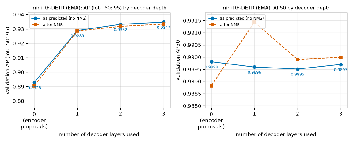
- Even without the decoder, AP is 0.8928. Just the 12 proposals produced directly by feature map cells come close to chapter 8's main model (0.8982). This is the earlier explanation, that the loss on the encoder proposals makes them "coarse detection results," showing up in the numbers.
- The decoder refines rather than finds. From 0 to 3 layers, AP rises by 0.042, 0.8928 → 0.9347, while AP50 stays the same, 0.9898 → 0.9897. AP50 measures "is there a roughly correct box," so finding the objects is already done at the proposal stage. What improves is the stricter IoU thresholds, including AP75 (0.9657 → 0.9762), that is, box precision.
- The first layer does most of the work. The per-layer gains are +0.036, +0.004, and +0.0015. Removing the last layer lowers AP by only 0.0015.
- Be sure to check the vertical axis of the right panel. The dotted orange line appears to bend sharply, but the vertical axis spans 0.988–0.992. The differences among the four points are all within 0.003 and are not meaningful.
- NMS brings no gain at any depth. AP after NMS is the same or slightly lower (−0.002 to 0.000). The number of pairs of predictions with score ≥ 0.5 overlapping at IoU above 0.5 goes 41 → 26 → 8 → 9, so the decoder reduces the small amount of duplication present at the proposal stage. This is consistent with chapter 7's explanation that the decoder's self-attention lets queries exchange information and remove duplicates.
- Note · Do not mix these with the paper's numbers
- The RF-DETR paper states that on COCO, removing the last decoder layer cuts latency by 10% and lowers mAP by 2. This chapter's "drops by 0.0015" was measured in the shapes world, where there are only 1–4 objects. The direction (using fewer layers is slightly less accurate) is the same, but the magnitude varies greatly with the data. Using the number of decoder layers as a knob continues in chapter 12.
In addition, per-class AP is 0.9729 for circles, 0.9071 for rectangles, and 0.9241 for triangles, with rectangles lowest. The order was the same in chapters 7 and 8 (the cause was not analyzed separately). In 484 of the 500 images, the number of predictions with score ≥ 0.5 exactly equals the number of ground-truth objects.
Prediction images and selected proposals
- Figure: Figure 11-9 Predictions (solid green, score ≥ 0.5) and ground truth (dotted white) for validation images 0–7. These are the same images as the prediction figures in chapters 7 and 8. Titles show "number of predictions / number of ground truths."
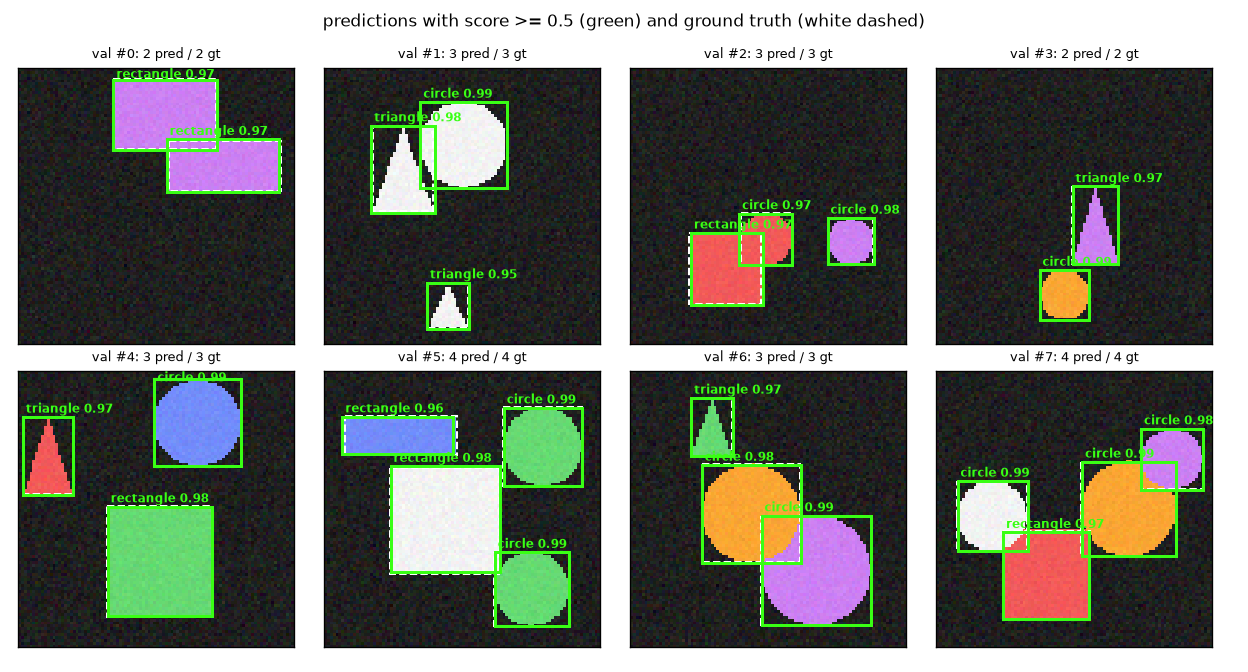
In all eight images, the number of predictions matches the number of ground truths, and the green boxes almost coincide with the white dotted ones. Scores are 0.95–0.99. Overlapping shapes (the rectangle and circle in image 2, the two circles in image 6, the three shapes in image 7) are also detected separately. However, these eight images are among the good cases. Of all 500 images, 484 have the right count, so sixteen images have missed or extra predictions.
- Figure: Figure 11-10 Two-stage query selection in practice (top: validation image 1, bottom: validation image 2). Far left: the proposal boxes of the 12 selected cells (side 0.05). Yellow marks cells of queries that end up with score ≥ 0.5, gray the rest; thin lines are the 12 × 12 cell boundaries and dotted white is the ground truth. Right four: how the predictions of the yellow queries come out at the encoder proposals (0 decoder layers) → decoder layer 1 → 2 → 3 (green, with class and score).
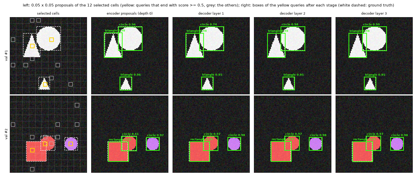
- Far left: every yellow cell lies inside an object, near its center. Gray cells are scattered over the background. Twelve cells are selected in an image with three objects, so nine are spare, and those queries end with low scores. The only thing that taught which cells to select is the classification loss on the encoder proposals.
- Second column: the encoder proposals alone already give boxes close to the ground truth. Starting from small proposals of side 0.05 (the small squares at far left), the two-stage box head enlarges them to object size in one go.
- The decoder refines the boxes slightly and corrects the scores. Look at the occluded circle in the bottom row. Half hidden behind a rectangle, it scored 0.41 at the encoder proposal stage but 0.97 after decoder layer 1. The proposal stage scores from the features of a single cell, whereas the decoder can reread the surroundings with cross-attention and compare against other queries with self-attention.
- Things do not always improve layer by layer. The circle in the top row goes 0.96 → 0.74 → 0.98 → 0.99, dipping briefly at layer 1 before recovering.
Do scores track box quality?
The experiment in chapter 3 showed that "even with the same boxes, a bad score ordering lowers AP," and summarized that a good score means a higher score for a more accurate box. Now the question deferred then can be checked: do the scores of a model trained with IA-BCE really track box IoU?
The method is as follows. For each ground-truth object in the validation set, pick one "prediction that found the object": among predictions of the same class with IoU ≥ 0.5, the one with the highest score (the prediction that becomes that object's true positive in chapter 3's scoring). Collect the (score, IoU) pairs of these predictions and see how closely the two move together.
As the measure of "moving together," Spearman's rank correlation is used. It is a correlation coefficient computed not from the values themselves but from their ranks. Rank the predictions 1st, 2nd, … by score and also by IoU, then express how well the two rankings agree as a number between −1 and +1. Identical rankings give +1, opposite rankings −1, and unrelated ones near 0. When there are no ties, it is computed simply from the rank differences \(\delta_k\) (\(P\) is the number of pairs and \(\delta_k\) is the difference between the two ranks of the \(k\)-th pair).
\(r_s = 1 - \frac{6 \sum_{k=1}^{P} \delta_k^{\,2}}{P\,(P^2 - 1)}\)
If five predictions have score ranks (1, 2, 3, 4, 5) and IoU ranks (2, 1, 3, 5, 4), the rank differences are (−1, 1, 0, −1, 1), the sum of squares is 4, and \(r_s = 1 - \frac{6 \times 4}{5 \times 24} = 1 - 0.2 = 0.8\). The ordinary (Pearson) correlation coefficient checks whether the values are linearly related, but here scores and IoUs are mostly bunched in 0.9–1.0 with a few far away, so it swings heavily on those few. What matters for AP is also the order of scores, not their values, so rank correlation is more suitable.
[점수와 IoU] 정답 객체마다 그 객체를 찾은 예측 (같은 클래스 · IoU ≥ 0.5 가운데 점수가 가장 높은 것) 의 점수와 IoU
  ch11 mini RF-DETR (IA-BCE)   | 찾은 객체 1261 / 1265 | 피어슨 +0.545 | 스피어만 +0.760 | 평균 점수 0.959 | 평균 IoU 0.953 | 평균 |점수 − IoU| 0.028
  ch08 Deformable DETR (focal) | 찾은 객체 1254 / 1265 | 피어슨 +0.509 | 스피어만 +0.358 | 평균 점수 0.915 | 평균 IoU 0.939 | 평균 |점수 − IoU| 0.071
- Figure: Figure 11-11 For each ground-truth object, the IoU (horizontal) and score (vertical) of the prediction that found it. Left: this chapter's model (IA-BCE). Right: chapter 8's model (focal loss). The orange line is the mean score per IoU bin, and the dotted gray line is the diagonal score = IoU.
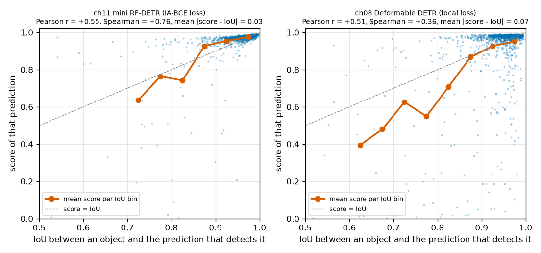
- On the left, the points cluster around the diagonal. The orange line (mean score per bin) hugs the diagonal above IoU 0.85. The mean score is 0.959, the mean IoU 0.953, and the mean absolute difference between them 0.028. Chapter 9's derivation, "the score is pulled toward the IoU," actually shows up in a trained model. For this model, a score of 0.95 roughly means "a box with an IoU of about 0.95."
- On the right, the points are spread vertically. At the right edge there is a long column of good boxes with IoU above 0.95 but scores of 0.2–0.8. The focal loss target is just 1 for a match and 0 otherwise, so there is no reason for the score to reflect how good the box is.
- The Spearman correlation is +0.760 vs. +0.358. For this chapter's model, ordering by score mostly gives the IoU order. This answers the question from chapter 3.
However, the two models in this comparison differ in both architecture and training length, so it cannot be concluded that this is "thanks to IA-BCE." A comparison that changes only the loss on the same architecture is needed. That is ablation (a) in the next section.
Reading the results: ablations
The main experiment shows only that "this setup as a whole works well." To know how much each component contributes, one has to retrain changing only one thing at a time. These are the ablations introduced in chapter 1. Five were run.
| Ablation | What changed | Baseline (base) | Topic in this chapter |
| (a) | Classification loss changed to focal loss | IA-BCE | Loss |
| (b) | Query groups reduced to 1 | 4 groups | Loss (Group DETR) |
| (c) | No EMA (scored with the regular model) | Scored with the EMA model | EMA |
| (d) | Windows set to 1 × 1 (all blocks use global attention) | 2 × 2 windows | Architecture from chapters 9 and 10 |
| (e) | Pretrained backbone; constant learning rate rule | Random backbone, official learning rate rule | Pretraining, layer-wise learning rate decay |
Experimental design and reading rules
- (a)–(d): 4,000 training images, 15 epochs, otherwise the same settings as the main experiment. Each was run three times with seeds 0, 1, and 2 (the seed changes the model's initial values and the data order).
- (c) was not trained separately. EMA takes no part in training, so scoring the EMA model and the regular model at the same epoch of a single base run directly compares "EMA on" and "EMA off."
- (e): explained separately below. Compared on 200 training images (3 seeds) and 4,000 (1 seed).
- The settings were fixed before looking at the results and were not changed afterward. At first a single seed was run, but the differences were too small to judge, so two more seeds were run with the same settings.
Before reading the numbers, decide how large a difference to trust. Differences smaller than the resolution of the measuring stick cannot be read. The resolution of this experiment can be gauged in two ways.
- Rerunning the same settings with the same seed gives different results. Two training runs of base (seed 0) ended at AP 0.9180 and 0.9182, which are close, but they diverged more along the way (0.3145 vs. 0.3113 at epoch 1, 0.8643 vs. 0.8688 at epoch 5). This is due to GPU nondeterminism.
- Changing the seed gives larger differences. The three seeds of base give 0.9180, 0.9210, and 0.9163, a range of 0.0047.
- Reading rule · Differences smaller than 0.005 are not read
- AP moves by about 0.005 even when nothing is changed. So in the tables of this section, if the difference between two settings is within 0.005, it is read as "no difference was seen." Even when the difference is larger, whether the direction is the same across the three seeds is checked as well.
Table of the four ablations
This table comes from the seed-0 run.
[절제 (a) – (d)] 학습 4000장, 15 에폭, 시드 1개 — 마지막 에폭의 검증 AP
  설정                                  | EMA 모델: AP    AP50   AP75  | 일반 모델: AP   AP50   AP75  | AP≥0.8 첫 에폭 (EMA) | 학습 시간
  base: IA-BCE, 4 groups, 2x2 windows   |          0.9180 0.9858 0.9695 |          0.9027 0.9828 0.9664 |          3           |   255초
  focal loss                            |          0.9144 0.9869 0.9681 |          0.9092 0.9880 0.9690 |          5           |   254초
  1 query group                         |          0.9156 0.9864 0.9712 |          0.8921 0.9885 0.9683 |          3           |   214초
  1x1 window (all global)               |          0.9166 0.9861 0.9667 |          0.9074 0.9859 0.9664 |          3           |   189초
  (c) EMA 유무는 base 한 번의 학습에서 EMA 모델과 일반 모델을 견준 것이다. 에폭별:
      에폭           1      2      3      5      7     10     15
      EMA  AP   0.3145 0.7172 0.8091 0.8643 0.8885 0.9053 0.9180
      일반 AP   0.2998 0.6859 0.7994 0.8500 0.8789 0.8875 0.9027
Here is the summary across the three seeds: the EMA model's validation AP at the last epoch and its difference from base with the same seed.
[절제 (a) – (d) 시드별 요약] 시드 [0, 1, 2] — 마지막 에폭의 EMA 모델 검증 AP 와, 같은 시드의 base 와의 차이
  설정                                  | 시드별 AP                | 평균   | base 와의 차이 (시드별)        | 차이의 평균
  base: IA-BCE, 4 groups, 2x2 windows   | 0.9180 0.9210 0.9163     | 0.9184 | +0.0000 +0.0000 +0.0000        | +0.0000
  focal loss                            | 0.9144 0.9103 0.9136     | 0.9128 | -0.0036 -0.0107 -0.0028        | -0.0057
  1 query group                         | 0.9156 0.9165 0.9158     | 0.9160 | -0.0024 -0.0045 -0.0005        | -0.0025
  1x1 window (all global)               | 0.9166 0.9251 0.9154     | 0.9190 | -0.0014 +0.0041 -0.0009        | +0.0006
  base, raw model (no EMA)              | 0.9027 0.9121 0.9000     | 0.9049 | -0.0153 -0.0089 -0.0163        | -0.0135
  AP50 의 시드 평균: base 0.9853 | focal loss 0.9834 | 1 query group 0.9860 | 1x1 window (all global) 0.9871
  AP75 의 시드 평균: base 0.9674 | focal loss 0.9679 | 1 query group 0.9701 | 1x1 window (all global) 0.9694
  점수와 IoU 의 상관 (스피어만), 시드별: IA-BCE +0.659 +0.631 +0.667 | focal +0.215 +0.318 +0.240
- Figure: Figure 11-12 Validation AP (left) and AP75 (right) for ablations (a)–(d), seed 0. Solid blue: base. Dotted orange: focal loss. Dash-dot green: 1 group. Dotted pink: 1 × 1 windows. Long-dashed yellow: base's regular model (no EMA).
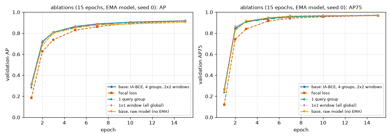
The first thing that stands out in Figure 11-12 is that the curves nearly overlap. Only the dotted orange line (focal loss) clearly lags early on (0.63 vs. 0.72 at epoch 2), and by epoch 15 all five curves gather at 0.90–0.92. Applying the reading rule to the "mean difference" column of the summary table splits them as follows.
| Ablation | Difference from base (seeds 0, 1, 2) | Mean | Reading |
| (c) No EMA | −0.0153, −0.0089, −0.0163 | −0.0135 | Clear. Larger than the resolution in all three seeds, with the same direction |
| (a) Focal loss | −0.0036, −0.0107, −0.0028 | −0.0057 | Same direction in all three seeds, but the size is around the resolution |
| (b) 1 group | −0.0024, −0.0045, −0.0005 | −0.0025 | Not seen (within the resolution) |
| (d) 1 × 1 windows | −0.0014, +0.0041, −0.0009 | +0.0006 | Not seen (signs are mixed too) |
Of the four, EMA has the largest effect and is the only one that is clear in all three seeds. Turning EMA off lowers AP by 0.0135 on average. This is larger than the final difference in the 60-epoch main experiment (0.0055), probably because at 15 epochs the regular model is still jittering more. The other three are examined in turn.
IA-BCE vs. focal loss
Looking at AP alone, the gain from IA-BCE is small. IA-BCE is higher in all three seeds, but by 0.0057 on average, and by less than 0.004 in two of the seeds. The seed means of AP50 are 0.9853 vs. 0.9834 and of AP75 0.9674 vs. 0.9679, so no difference. The consistent difference is in early speed: the first epoch to reach AP 0.8 is 3 for IA-BCE and 5 for focal in all three seeds.
Looking at the relationship between score and IoU, however, tells a different story. This time the comparison is between two models with the same architecture and training length, differing only in the classification loss.
[절제 (a)] 점수와 IoU — 같은 모델 구조, 분류 손실만 다름 (정답 객체마다 그 객체를 찾은 예측의 점수와 IoU)
  IA-BCE loss (base)           | 찾은 객체 1258 / 1265 | 피어슨 +0.569 | 스피어만 +0.659 | 평균 점수 0.935 | 평균 IoU 0.945 | 평균 |점수 − IoU| 0.035
  focal loss                   | 찾은 객체 1262 / 1265 | 피어슨 +0.429 | 스피어만 +0.215 | 평균 점수 0.808 | 평균 IoU 0.945 | 평균 |점수 − IoU| 0.140
- Figure: Figure 11-13 Two models from the same mini RF-DETR trained for 15 epochs (seed 0). Left: IA-BCE. Right: focal loss. The format is the same as Figure 11-11 (horizontal IoU, vertical score, orange line the mean score per bin, dotted gray line score = IoU).
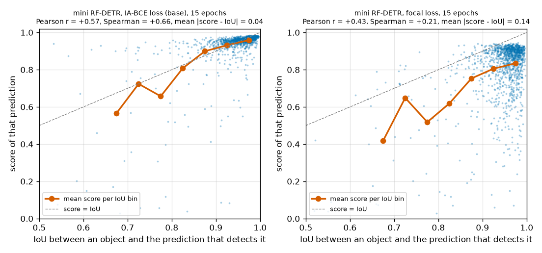
| Seed 0 | Seed 1 | Seed 2 | |
| Spearman correlation: IA-BCE / focal | +0.659 / +0.215 | +0.631 / +0.318 | +0.667 / +0.240 |
| Mean score (mean IoU): IA-BCE | 0.935 (0.945) | 0.926 (0.946) | 0.930 (0.943) |
| Mean score (mean IoU): focal | 0.808 (0.945) | 0.783 (0.945) | 0.788 (0.945) |
| Mean \(|\text{score} - \text{IoU}|\): IA-BCE / focal | 0.035 / 0.140 | 0.040 / 0.165 | 0.036 / 0.159 |
- The Spearman correlation drops from +0.65 to +0.26 on average over the three seeds. The size is far beyond the resolution, and it holds for all three seeds. Changing only the loss greatly changes "how well the score tracks box quality." This means the earlier comparison with the chapter 8 model (+0.76 vs. +0.36) was not due only to the architectural difference.
- The boxes are equally good. The mean IoU is 0.945 for both losses; only the scores differ. The IA-BCE model's mean score of 0.93 is nearly equal to its mean IoU of 0.945 (left panel: around the diagonal), while the focal model's mean score is low at 0.78–0.81 regardless of IoU and spread widely over 0.6–0.95 (right panel).
The meaning of the score changed this much, so why does AP change only a little? Chapter 3's experiment gives the answer. Score ordering matters when true positives and false positives are mixed. In this data each image has only 1–4 objects, and most predicted boxes exceed IoU 0.9. Few boxes would become false positives even at strict thresholds, so there is little to gain from fixing the order. The thread set up in chapter 3 is thus only half resolved by this experiment: "IA-BCE aligns scores with box quality" is clearly confirmed, while "and therefore AP rises" is only weakly confirmed.
- Note · Values the paper reports on COCO
- Table 2 of the LW-DETR paper reports that on COCO (12-epoch setting), adding the IoU-aware classification loss raises mAP by 0.7, from 34.7 to 35.4. That is on data with many objects per image and uneven box quality. It is a different experiment from this chapter's value (shapes world, +0.006 on average), so do not put them side by side to compare magnitudes. Also, the focal loss in this ablation has a coefficient of 1 (turning off only IA-BCE in the official implementation). A coefficient of 2 might give different results, but that was not tried.
Query groups and number of windows
(b) Group DETR. The differences between 4 groups and 1 group are −0.0024, −0.0045, and −0.0005. The 4-group setting is higher in all three seeds, but the differences are below the resolution. The epoch at which AP 0.8 is reached is also the same, 3. The effect of Group DETR was not seen in this experiment. Some plausible reasons can be considered (not checked separately).
- With 12 queries and 1–4 objects, about a fifth of the queries get a match even with a single group. The official setting has 300 queries, so the fraction of queries that get a match is much lower, and adding matches by adding groups is more pressing there.
- The losses on the encoder proposals and the three decoder layers already provide training signal at four sites.
- Compared with the official 13 groups, 4 groups is a small change in the first place.
Table 2 of the LW-DETR paper reports that on COCO, adding Group DETR ("more supervision") raises mAP by 3.0, from 35.4 to 38.4. What was a large effect in the paper's table did not appear in this small experiment. This experiment does not refute the paper: COCO with 300 queries and dozens of objects and the shapes world with 12 queries and four objects are different situations. Still, it is worth remembering that the effect of a technique varies with the data and scale. Training with 1 group was about 10% faster for seeds 1 and 2.
(d) Window attention. The differences between 2 × 2 windows (base) and all blocks switched to global attention are −0.0014, +0.0041, and −0.0009, with mixed signs. Window attention did not cost accuracy. The purpose of window attention is not to raise accuracy but to reduce computation (chapter 9), so "no difference" is the desired result. For reference, in Table 2 of the LW-DETR paper, adding window attention reduces compute from 23.0 to 16.6 GFLOPs while mAP drops slightly from 36.0 to 34.7. That drop was not seen in this experiment either.
[절제 (d) 보충] 윈도 수를 추론 때만 바꿔 채점 (EMA 모델)
    base: IA-BCE, 4 groups, 2x2 windows   → num_windows=1: AP 0.9169 | num_windows=2: AP 0.9180 | num_windows=3: AP 0.9174
    1x1 window (all global)               → num_windows=1: AP 0.9166 | num_windows=2: AP 0.9118 | num_windows=3: AP 0.8937
One more thing was observed as a bonus: the results above, scoring trained models with the number of windows changed only at inference. The model trained with 2 × 2 windows keeps the same AP when switched to 1 × 1 or 3 × 3 windows at inference (0.9169, 0.9180, 0.9174; the other two seeds are also within ±0.002). Conversely, the model trained only with global attention drops when windows are introduced (for seed 0, −0.005 with 2 × 2 and −0.023 with 3 × 3; over the three seeds, −0.012 to −0.023 with 3 × 3). A backbone trained with windows mixed in tolerates changes in the number of windows better, which comes up again in chapter 12, where the number of windows is used as a knob.
Backbone pretraining experiment: masked image modeling
The last ablation, (e), checks two big themes of this chapter together: pretraining and layer-wise learning rate decay. The paper's claim is that "a pretrained backbone helps on small datasets," and layer-wise decay was the mechanism for protecting that backbone. To test the same thing in the shapes world, a pretrained backbone is needed first.
Rather than imitating DINOv2 wholesale, a method that takes only a few lines to implement was chosen: masked image modeling (MIM). Some patches of the image are hidden, and the model must predict the pixels of the hidden patches from the visible ones alone. It is self-supervised learning that needs no labels (chapter 6). To fill in the hidden areas, the model has to know how far the edges and colors of shapes extend, so the hope is that useful features emerge in the process. LW-DETR's backbone pretraining (CAEv2) belongs to this family. DINOv2, as seen in chapter 6, uses a different approach, self-distillation.
ch11_train.py · pretrain — This long code is collapsed in the original and is not reproduced here. It is in the pretrain region of code/ch11_train.py.
-
patchify: converts an image(B, 3, H, W)into(B, h·w, 3·p·p), flattening each patch's pixels into one row. With patch size 8, one patch is \(3 \times 8 \times 8 = 192\) numbers. -
mask: a boolean array(B, h·w)deciding for each patch, with probability 0.5, whether to "hide" it. The patch embeddings at hidden positions are replaced by a mask token learned inside the backbone. - For each cell of the backbone's last feature map
(B, C, h, w), a single linear layer predicts that patch's 192 pixels, and the loss is L1 measured only on hidden patches.
The design is as follows.
- Pretraining data: 8,000 shapes-world images (seed 100). They do not overlap with the training or validation images, and the labels are not read. 30 epochs (1,860 steps), batch 128.
- Small-data experiment: detection training images reduced to 200, 100 epochs (600 steps). Four settings, backbone {random, pretrained} × learning rate {official rule, constant}, each with three seeds.
- Large-data experiment: random vs. pretrained with 4,000 training images, 15 epochs, and the official learning rate rule (1 seed).
- "Constant" is the orange bars in Figure 11-4, the setting where every parameter's learning rate is \(2 \times 10^{-4}\).
[절제 (e)] 백본 사전 학습: 라벨 없는 그림 8000장 (seed 100), 마스크 그림 모델링 30 에폭, 배치 128, AdamW lr 5e-4, 가린 비율 0.5
  사전 학습 에폭   1 | 가린 패치의 L1 손실 0.6457
  사전 학습 에폭   2 | 가린 패치의 L1 손실 0.4096
  사전 학습 에폭   3 | 가린 패치의 L1 손실 0.4005
  사전 학습 에폭   5 | 가린 패치의 L1 손실 0.3961
  사전 학습 에폭  10 | 가린 패치의 L1 손실 0.3871
  사전 학습 에폭  15 | 가린 패치의 L1 손실 0.3809
  사전 학습 에폭  20 | 가린 패치의 L1 손실 0.3765
  사전 학습 에폭  25 | 가린 패치의 L1 손실 0.3739
  사전 학습 에폭  30 | 가린 패치의 L1 손실 0.3669
  사전 학습 205초 (1860 스텝), 손실 0.6457 → 0.3669
- Figure: Figure 11-14 Reconstruction examples from the pretrained backbone (six validation images not used in pretraining). Top: originals. Middle: inputs with 50% of patches hidden (gray marks hidden areas). Bottom: hidden patches filled in with the model's predictions.
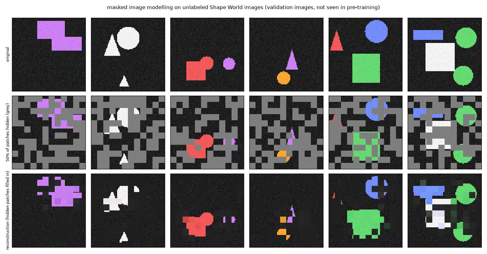
Figure 11-14 shows how weak this pretraining is. Inside shapes where neighboring patches are visible, the color is filled in, but the filled shapes are blocky at the patch level. Where the hidden area is large, many places are simply filled with background. The circle in the second image has its left side cut off, and the orange circle in the fourth image is left as a few square fragments. The loss also dropped to 0.41 within 2 epochs and was still descending slowly, reaching 0.37 at epoch 30. This point comes up again when interpreting the results below.
Results of the pretraining experiment
  [작은 데이터 200장] 마지막 에폭의 EMA 모델 검증 AP (시드 3개)
    설정                            | 시드별 AP                | 평균   | 최소 – 최대     | AP50 평균 | AP75 평균
    random init, official lr rule   | 0.6676 0.6877 0.6703     | 0.6752 | 0.6676 – 0.6877 | 0.8680    | 0.7792
    random init, flat lr            | 0.7124 0.7315 0.7071     | 0.7170 | 0.7071 – 0.7315 | 0.8920    | 0.8132
    pre-trained, official lr rule   | 0.6938 0.6965 0.6681     | 0.6861 | 0.6681 – 0.6965 | 0.8783    | 0.7853
    pre-trained, flat lr            | 0.7038 0.7125 0.6840     | 0.7001 | 0.6840 – 0.7125 | 0.8787    | 0.7953
    사전 학습의 이득 (평균 AP): 공식 학습률 규칙 +0.0109, 일정한 학습률 -0.0169
    공식 학습률 규칙의 이득 (평균 AP): 사전 학습 백본 -0.0140, 무작위 초기화 -0.0418
  [큰 데이터 4000장, 15 에폭, 시드 1개, 공식 학습률 규칙] EMA 모델의 검증 AP
      에폭               1      2      3      5      7     10     15
      무작위 초기화 0.3113 0.7221 0.8201 0.8688 0.8869 0.9059 0.9182
      사전 학습     0.3018 0.6940 0.8011 0.8520 0.8801 0.9047 0.9177
  사전 학습의 이득 (공식 학습률 규칙, 마지막 에폭 AP): 200장 +0.0109 (0.6752 → 0.6861), 4000장 -0.0005 (0.9182 → 0.9177)
- Figure: Figure 11-15 Left: pretraining loss (L1 on hidden patches). Middle: validation AP with 200 training images (EMA model). Lines are the mean over three seeds, bands the min–max. Solid blue: random + official rule. Dotted orange: random + constant. Dash-dot green: pretrained + official rule. Dotted pink: pretrained + constant. Right: final AP under the official learning rate rule, blue for random and green for pretrained.
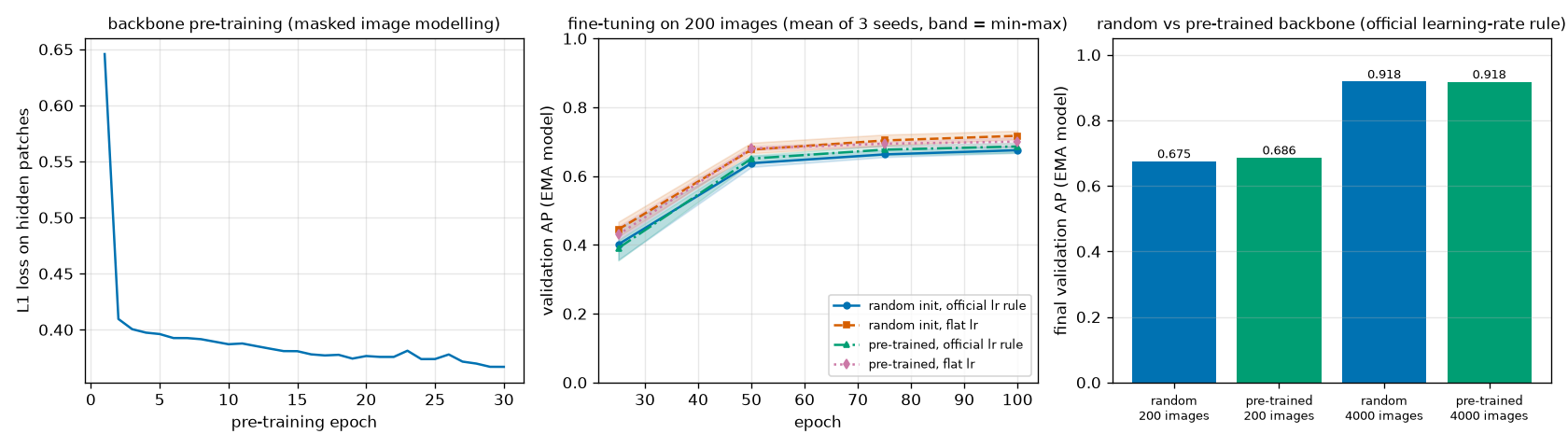
| 200 training images, final AP (mean and range over three seeds) | Official learning rate rule | Constant learning rate | Gain/loss from the official rule |
| Randomly initialized backbone | 0.6752 (0.6676 – 0.6877) | 0.7170 (0.7071 – 0.7315) | −0.0418 |
| Pretrained backbone | 0.6861 (0.6681 – 0.6965) | 0.7001 (0.6840 – 0.7125) | −0.0140 |
| Gain/loss from pretraining | +0.0109 | −0.0169 |
The results are reported as they are. The benefit of backbone pretraining was not reproduced in this mini experiment.
- 200 training images, official learning rate rule: random 0.6752, pretrained 0.6861. Pretrained is 0.011 higher, but the seed ranges of the two settings overlap (0.6676–0.6877 and 0.6681–0.6965). The blue and green bands in the middle of Figure 11-15 overlap.
- 200 training images, constant learning rate: random 0.7170, pretrained 0.7001. This time pretrained is 0.017 lower.
- The best of the four settings is "random initialization + constant learning rate" (the dotted orange line is on top in the middle panel).
- 4,000 training images: 0.9182 vs. 0.9177, no difference. Early on, pretrained is actually slower (0.7221 vs. 0.6940 at epoch 2, 0.8688 vs. 0.8520 at epoch 5).
One thing did match expectations: the rightmost column of the table. The cost of the official learning rate rule (low backbone learning rate and layer-wise decay) is smaller for the pretrained backbone. Relative to a constant learning rate, the cost is 0.042 for the random backbone and 0.014 for the pretrained one. The rule "change the backbone only a little" does not suit a random backbone with a lot to change, and is less harmful to a backbone that has already learned something. This is consistent with what layer-wise decay presupposes. Even so, with this budget (600 steps) a constant learning rate was better for both backbones. This is also a clue about this chapter's main experiment: it used the official rule on a random backbone, so a constant learning rate might have done better (this was not measured with 4,000 images and 60 epochs).
Why was there no visible benefit?
What follows are hypotheses. None was checked with a separate experiment. The settings were also not changed and rerun after seeing the results, to avoid tweaking settings until the desired conclusion appears.
- The pretraining is weak. It is 1,860 steps of masked image modeling, and as seen in Figure 11-14, the reconstruction is at the level of blocky color filling. DINOv2 is a model trained on 142 million images; the number of images alone differs by more than ten thousand times.
- The pretraining data has the same distribution as the task. It is 8,000 shape images from the same generator. The advantage of real pretraining lies in "having seen a much wider world than the target data in advance," and that is missing here. Moreover, the features this task needs (color blobs and edges) are learned quickly from just 200 labeled images, about 500 objects. A random backbone reaches AP 0.72 in 600 steps.
- The task is easy and the backbone is small. 200 images may not be "very little data" for this task. Trying 20–50 images was not done.
- The objectives differ. The last layers of a backbone trained to reconstruct pixels are tuned for reconstruction. Using it for detection requires substantial relearning, which 600 steps and a low backbone learning rate may not have allowed. This explanation is consistent with pretrained being slower early in the 4,000-image experiment, and with pretraining actually hurting under a constant learning rate.
- This is not a comparison of converged values. In the 200-image experiment, AP was still rising at 100 epochs (it rose in eleven of twelve cases between epochs 75 and 100).
What this experiment tells us is narrow: "weak pretraining on the same distribution did not help on this easy task." That is all. Longer pretraining, a DINO-style objective, fewer labels, and a frozen-backbone comparison were not tried. So this neither refutes nor confirms the paper's claim.
Real weights and the paper's evidence
Then what does the claim "pretraining matters" rest on? There are three kinds of evidence, and since they are different, they are listed separately.
| Evidence | What was compared | Result |
| This chapter's mini experiment (shapes world, run directly) | Weak MIM-pretrained backbone vs. random backbone | No visible benefit (200 images +0.011 / −0.017, 4,000 images −0.0005) |
| Experiment in chapter 14 (shapes world, run directly, real RF-DETR Nano weights) | Starting from official pretrained weights vs. fully random initialization; 1,000 training images, same settings | Validation AP at the same epoch 3: 0.9816 vs. 0.7749. Pretrained already at 0.9476 after epoch 1 |
| The papers (COCO) | RF-DETR Tables 5 and 6: switching the backbone to DINOv2. LW-DETR Table 5: with or without Objects365 pretraining | +2.0 AP (51.6 → 53.6, 52.3 → 54.3). +4.4 to +6.6 mAP (depending on size) |
The second row matters. It is a comparison in the same shapes world, with the same package and the same settings, changing only the starting point. Scoring the two models trained in chapter 14 on the test set gives AP 0.9830 (starting from pretrained, 5 epochs) and 0.7738 (random initialization, 3 epochs). The epoch counts differ, so the same-epoch comparison is the table's 0.9816 vs. 0.7749. Either way, the gap exceeds 0.2, an order of magnitude beyond the 0.01 differences debated in this chapter's mini experiment.
The difference between the two experiments is the quality and breadth of the pretraining. The chapter 14 weights went through self-supervised learning on more than 100 million photos and had already learned detection on Objects365. Even without ever seeing shapes, they already know "how to put boxes around objects." This chapter's pretraining was a few minutes of practicing pixel filling on 8,000 shape images. The two are too different to share the same word "pretraining."
- Key points · What to take from the ablations
- First measure the resolution of the measuring stick (rerun variation with the same settings, variation across seeds), and do not read differences smaller than that.
- Clear in this chapter's experiments: the benefit of EMA (turning it off costs AP −0.0135), and IA-BCE aligning scores with IoU (Spearman +0.65 vs. +0.26).
- Not seen: Group DETR, number of windows (no accuracy cost), and the benefit of weak pretraining.
- "Not seen" is not "no effect." It means smaller than the resolution on this data at this scale. It should be read together with the effects the papers report on COCO and the chapter 14 results measured with real weights.
Mapping to real-world training
This table gathers how the TrainConfig defaults you encounter when fine-tuning a real model with the rfdetr package in chapter 14 connect to the concepts in this chapter. The loss coefficients, number of groups, and whether to use IA-BCE live in the model config rather than the training config.
| Setting name | Default | Concept in this chapter |
| | 1e-4 | Base learning rate \(\eta\). The projector, heads, and query embeddings learn at this rate |
| | 1.5e-4 | Backbone base learning rate \(\eta_{\text{enc}}\) |
| | 0.8 | Layer-wise learning rate decay rate \(\lambda\) |
| | 0.7 | Per-component decay rate \(\rho\) (once for the decoder, twice for the backbone) |
| | 1e-4 | AdamW weight decay (chapter 4) |
| | 4, 1 | Batch size and gradient accumulation. Their product is the effective batch size. The package documentation recommends an effective batch of 16 |
| | 100 | The learning rate is constant, so changing this does not change the learning rate curve |
| | 0 | No warmup |
| | 0.1 | Gradient clipping limit \(c_{\max}\) |
| | True, 0.993, 100 | EMA, its decay \(d\), and the warmup \(\tau\) |
| | per-batch, True | Per-batch multi-resolution training and the expanded resolution range |
| | 0.0 | Drop path (below). Not used by default |
| | 1, 5, 2 | Loss coefficients |
| | 13, True | Number of query groups \(G\); IA-BCE as the classification loss |
One name in the table was not covered in this chapter. Drop path (stochastic depth) is a regularization technique that randomly skips an entire residual branch during training. For a residual block \(y = x + F(x)\) (chapter 4), it sets \(F(x)\) to 0 with probability \(q\) and otherwise scales it up to \(F(x)/(1 - q)\) to keep the expectation the same. The effect is like training a network of a different depth each time. RF-DETR's default is 0, meaning it is not used. The experiments in this tutorial do not use it either.
Read in one line, the defaults follow this chapter's table of contents exactly: AdamW, learning rate 1e-4 held constant to the end, no warmup, gradients clipped at 0.1, the backbone slowed by 0.8× per layer, and evaluation with EMA weights at decay 0.993. In chapter 14, a real model is trained with these settings, and the nine loss names and the smallest learning rate \(3.23 \times 10^{-6}\) that appear in the log are reread with this chapter's formulas.
Summary
- Full loss: at the encoder proposals and each decoder layer, Hungarian matching is done per query group at each site (cost 2 · focal form + 5 · L1 + 2 · (−GIoU)), and IA-BCE, L1, and \((1 - \operatorname{GIoU})\) are divided by number of ground truths × number of groups and added with coefficients 1, 5, and 2. The number of loss values is (number of decoder layers + 1) × 3, independent of the number of groups.
- The encoder-proposal loss is the only signal that teaches query selection, and the per-layer losses make it possible to remove decoder layers at inference.
- Scheduler-free training: a cosine schedule's learning rate is determined only by \(n / n_{\text{end}}\), so the training length must be known in advance. RF-DETR keeps the learning rate constant to the end and uses no warmup.
- Gradient accumulation: adding the gradients of several small batches produces the gradient of a large batch. The equality holds only without batch normalization.
- Gradient clipping: \(\mathbf{g} \leftarrow \mathbf{g} \cdot \min(1,\ c_{\max} / \lVert \mathbf{g} \rVert)\), \(c_{\max} = 0.1\). In this model it applies at every step, making the magnitude of the gradient fed to Adam the same at every step.
- EMA: \(\theta_{\text{ema}} \leftarrow d\,\theta_{\text{ema}} + (1 - d)\,\theta\). It is an average over roughly the last \(1/(1 - d)\) steps, about 143 steps for \(d = 0.993\). The decay rises from near 0 as \(d\,(1 - e^{-n/\tau})\). It takes no part in training and is used for evaluation and saving.
- Layer-wise learning rate decay: the learning rate of a backbone parameter is \(\eta_{\text{enc}} \cdot \lambda^{L + 1 - i} \cdot \rho^2\). In Nano, the bottom block learns at 1/11.6 the rate of the top block, and the embeddings at 1/31 the rate of the heads. It is a mechanism for protecting a pretrained backbone.
- Augmentation is limited to horizontal flips and random crops, with per-batch multi-resolution. Pretraining has three stages: DINOv2 → Objects365 → target data.
- Mini experiment: AP 0.9347 (EMA) at 60 epochs. EMA beat the regular model in nineteen out of twenty scorings, the encoder proposals alone reached AP 0.8928, and the Spearman correlation between score and IoU for the IA-BCE model was +0.76. The effects of Group DETR, the number of windows, and weak pretraining were not visible at this experiment's resolution.
In this chapter, the mini RF-DETR was trained with one architecture, one resolution, and three decoder layers. Yet, as seen when measuring AP by number of layers, this model already contains "0-layer," "1-layer," and "2-layer" detectors within it. It was also seen that AP holds when the number of windows is changed only at inference. If several models can be extracted from weights trained once, could the same be done not only for the number of decoder layers but also for resolution, patch size, number of windows, and number of queries? Choosing, among the thousands of models extracted this way, the most accurate one for a given latency is the neural architecture search in the title of the RF-DETR paper. In chapter 12, this is tried hands-on by adding "randomly change the architecture at every step" to this chapter's training loop.
Review questions
- Question 1 · Counting loss terms
- RF-DETR Medium has 4 decoder layers and trains with 300 queries and 13 groups. (1) How many loss values appear in the training log? (2) How many queries are there in total during training? (3) How many times does the Hungarian solver run in one training step on a batch of 8 images? (4) If the batch has 40 ground-truth objects in total, what is
num_boxes? - Answer. (1) There are \(4 + 1 = 5\) sites (4 decoder layers + encoder proposals), with three values per site, so \(5 \times 3 = 15\). The number of groups does not change this.
- (2) \(13 \times 300 = 3{,}900\).
- (3) 5 sites × 8 images × 13 groups = 520 times.
- (4) Number of ground truths × number of groups \(= 40 \times 13 = 520\).
- Question 2 · Computing the loss by hand
- An image has one ground truth (a circle), and one group has two queries. Query 0 is matched to the ground truth; its probability for circle is \(0.5\), its box IoU is \(0.9\), its GIoU is also \(0.9\), and its L1 distance is \(0.04\). Of the remaining five cells, only query 1's circle cell has probability \(0.2\), and the others are small enough to treat as 0. (1) Find the target \(t\) (\(0.5^{0.25} = 0.8409\), \(0.9^{0.75} = 0.9240\)). (2) Find the three losses at this site and their weighted sum. (3) In which direction does the logit of the matched cell move?
- Answer. (1) \(t = 0.8409 \times 0.9240 = 0.7770\).
- (2) Matched cell: \(-t \log 0.5 - (1 - t)\log 0.5 = \log 2 = 0.6931\). With \(\hat{p} = 0.5\) the two logarithms are equal, so it is \(\log 2\) regardless of \(t\). Query 1's circle cell: \(0.2^2 \times (-\log 0.8) = 0.04 \times 0.2231 = 0.0089\). Since
num_boxes\(= 1 \times 1 = 1\), \(\mathcal{L}_{\text{cls}} = 0.6931 + 0.0089 = 0.7020\). \(\mathcal{L}_{\text{L1}} = 0.04\), \(\mathcal{L}_{\operatorname{GIoU}} = 1 - 0.9 = 0.1\). The weighted sum is \(0.7020 + 5 \times 0.04 + 2 \times 0.1 = 0.7020 + 0.2 + 0.2 = 1.1020\). - (3) The gradient with respect to the logit is \(\hat{p} - t = 0.5 - 0.777 = -0.277\), negative, so the logit moves up, raising the score from 0.5 toward the IoU.
- Question 3 · Gradient clipping
- Norm clipping is applied with limit \(c_{\max} = 0.1\). (1) What happens to \(\mathbf{g} = (0.6,\ 0.8,\ 0)\)? (2) And to \(\mathbf{g} = (0.02,\ 0.01,\ 0.02)\)? (3) If the optimizer is SGD with learning rate \(10^{-4}\), what is the maximum distance the weight vector can move in one step? (4) Compared with "clipping each component separately to \([-0.1, 0.1]\)," what is the advantage of norm clipping?
- Answer. (1) \(\lVert \mathbf{g} \rVert = \sqrt{0.36 + 0.64} = 1\). \(s = \min(1,\ 0.1/1) = 0.1\), so it becomes \((0.06,\ 0.08,\ 0)\), with length 0.1.
- (2) \(\lVert \mathbf{g} \rVert = \sqrt{0.0004 + 0.0001 + 0.0004} = 0.03 \le 0.1\), so it is unchanged.
- (3) \(\eta \cdot c_{\max} = 10^{-4} \times 0.1 = 10^{-5}\).
- (4) The direction does not change. Component-wise clipping shrinks only the large components, changing the gradient's direction. Clipping the vector from (1) component-wise gives \((0.1,\ 0.1,\ 0)\), turning the 3 : 4 ratio into 1 : 1.
- Question 4 · Length of an EMA
- Consider an EMA with decay \(d = 0.99\) (no warmup). (1) Roughly how many recent steps is it an average over? (2) With \(\theta_{\text{ema}} = 0.50\) and \(\theta = 0.60\), what is the value after one update? (3) After 100 steps, what weighting does the initial value of the EMA hold (\(0.99^{100} = 0.366\))? (4) How many steps does it take for the weighting of a given step's weights to halve (\(\ln 0.5 = -0.6931\), \(\ln 0.99 = -0.01005\))?
- Answer. (1) \(1/(1 - 0.99) = 100\) steps.
- (2) \(0.99 \times 0.50 + 0.01 \times 0.60 = 0.495 + 0.006 = 0.501\).
- (3) \(d^{100} = 0.366\), that is, 37%. Even after \(1/(1 - d)\) steps, more than a third of the initial value remains. This is why decay warmup is needed.
- (4) \(n = \ln 0.5 / \ln 0.99 = 0.6931 / 0.01005 = 69.0\) steps.
- Question 5 · Decay warmup
- Using the official implementation's formula \(d_n = 0.993\,(1 - e^{-n/100})\): (1) Find the decay and the averaging length \(1/(1 - d_n)\) at \(n = 50\) (\(e^{-0.5} = 0.6065\)). (2) If \(d = 0.993\) had been used from the start without warmup, in training with 125 steps per epoch, what weighting would the untrained weights hold in the EMA model after one epoch (\(0.993^{125} = 0.416\))? Predict how that EMA model would score.
- Answer. (1) \(d_{50} = 0.993 \times (1 - 0.6065) = 0.993 \times 0.3935 = 0.3907\). The averaging length is \(1/(1 - 0.3907) = 1.64\) steps. This matches "스텝 50: 0.3907" (step 50: 0.3907) in the lab output.
- (2) 0.416, that is, 42%. 42% of the EMA weights would be the random initial values and the rest weights from early in training, so its AP would be far worse than the regular model at epoch 1. With warmup, the decay of the first update is 0.0099, so the weighting of the initial values drops below 1% immediately. In this chapter's experiment, the EMA model at epoch 1 (0.3085) did not fall behind the regular model (0.3011).
- Question 6 · Layer-wise learning rate decay
- For RF-DETR Nano (12 blocks, \(L = 13\), \(\eta = 10^{-4}\), \(\eta_{\text{enc}} = 1.5 \times 10^{-4}\), \(\lambda = 0.8\), \(\rho = 0.7\)): (1) Find the learning rate of block 8 (\(0.8^5 = 0.32768\)). (2) What is the decoder's learning rate, and what multiple of it is block 0's learning rate (\(4.04 \times 10^{-6}\))? (3) If \(L\) had been set to the number of blocks, 12, what would block 11's learning rate be? Compare it with the value in the public code.
- Answer. (1) The exponent is \(L - j = 13 - 8 = 5\). \(1.5 \times 10^{-4} \times 0.49 \times 0.32768 = 7.35 \times 10^{-5} \times 0.32768 = 2.41 \times 10^{-5}\).
- (2) The decoder is \(\eta \cdot \rho = 7.0 \times 10^{-5}\). Block 0 is \(4.04 \times 10^{-6} / 7.0 \times 10^{-5} = 0.058\) times that, about 1/17.
- (3) The exponent becomes \(12 - 11 = 1\), giving \(7.35 \times 10^{-5} \times 0.8 = 5.88 \times 10^{-5}\). The actual value in the public code is \(7.35 \times 10^{-5} \times 0.64 = 4.70 \times 10^{-5}\). Counting \(L\) one higher makes every block of the backbone learn 0.8× slower. This is a difference that cannot be known from the paper's text alone; it requires reading the code.
- Question 7 · Cosine schedule
- A cosine schedule with \(\eta_0 = 2 \times 10^{-4}\) and \(\eta_{\min} = 0\) was set up with \(n_{\text{end}} = 40\) epochs. (1) Find the learning rate at epochs 10 and 30 (\(\cos(\pi/4) = 0.7071\)). (2) At epoch 20, validation AP stopped improving and training was stopped. What was the learning rate at that point? (3) What would have been different with RF-DETR's approach in the same situation?
- Answer. (1) Epoch 10: \(\tfrac{1}{2}(1 + \cos(\pi/4)) = 0.8536\), so \(1.71 \times 10^{-4}\). Epoch 30: \(\tfrac{1}{2}(1 + \cos(3\pi/4)) = \tfrac{1}{2}(1 - 0.7071) = 0.1464\), so \(0.29 \times 10^{-4}\).
- (2) Exactly halfway, so \(\tfrac{1}{2}\eta_0 = 1.0 \times 10^{-4}\). Training ended with the learning rate still at half its initial value. It is hard to tell whether "AP stopped improving" means training was done or the learning rate was too high.
- (3) The learning rate is the same from start to finish, so the model at epoch 20 is the same whether training stops at 20 or continues to 40. The weights at the stopping point will be jittering, but evaluation uses the EMA weights averaged over roughly the last 143 steps. There is no need to fix the training length in advance.
- Question 8 · Reading the ablations
- (1) This chapter's ablation (c) did not run a separate training with EMA turned off. Explain why that is acceptable. Could the same approach be used for DINO in chapter 6? (2) Adding some technique raised AP by +0.003, +0.004, and +0.002 over three seeds. If the range from rerunning the same settings with different seeds is 0.005, how should this be reported? (3) In ablation (a), the AP difference between IA-BCE and focal loss was small, but the Spearman correlation differed greatly. Explain why the two results are not contradictory.
- Answer. (1) RF-DETR's EMA model takes no part in training. The forward pass, loss, and backward pass use only the regular model, so the regular model's weights are identical whether EMA is on or off. Therefore the score of the regular model from a single run is exactly the result of "training with EMA off." This does not work for DINO: the output of the EMA-built teacher is the student's training target, so changing the EMA changes training itself.
- (2) Report both that the direction is the same in all three seeds and that the size is smaller than the rerun range. The honest report is "there may be an effect, but it was not confirmed at this experiment's resolution." Writing the mean +0.003 simply as a "performance improvement" is not acceptable.
- (3) The Spearman correlation checks whether, among the "predictions that found objects," the order of scores matches the order of IoUs. AP checks how true positives and false positives are mixed when ordered by score. In this data, most predictions exceed IoU 0.9 and are true positives at every threshold. Reordering true positives among themselves does not change AP, so AP can stay almost the same even when the order differs a lot.
See also
Favorite site
- 11. Training RF-DETR
- code/ch11_train.py
- RF-DETR: Neural Architecture Search for Real-Time Detection Transformers (arXiv:2511.09554)
- LW-DETR: A Transformer Replacement to YOLO for Real-Time Detection (arXiv:2406.03459)
- DINOv2: Learning Robust Visual Features without Supervision (arXiv:2304.07193)
- GitHub - roboflow/rf-detr