RF-DETR:Tutorial:10-Architecture
lastmod 2026-11-18created 2026-11-189 edits
RF-DETR architecture is chapter 10 of the RF-DETR tutorial. It assembles the ViT and DINOv2 from chapter 6, set prediction from chapter 7, deformable attention and the two-stage scheme from chapter 8, and window attention, the projector and box reparameterization from chapter 9 into a single model, then follows from start to finish how the tensor shapes change as one image goes in and 300 boxes come out. It counts by hand how many of the 30.47 million parameters sit in each component and checks the total against the real model, always places values measured on the real RF-DETR Nano side by side with the mini RF-DETR of the shape world, and points out where the paper's description differs from what the released code actually does. Training the assembled architecture is the subject of chapter 11.
- Original: 10. RF-DETR Architecture
- Practice code:
code/ch10_rfdetr_model.py. No training; it builds the mini RF-DETR (MiniRFDETR), traces tensor shapes step by step, counts parameters, and checks properties that follow from the architecture. About 35 seconds on a laptop GPU (--quick: about 15 seconds on CPU). The RF-DETR Nano comparison requires therfdetrpackage. Reading time of the original about 100 minutes, difficulty ★★★★☆. - Previous: 09. Real-time DETR: RT-DETR and LW-DETR / Next: 11. Training RF-DETR
- What this chapter covers
- Splitting the RF-DETR forward pass into eight steps and stating the tensor shape at each step for RF-DETR Nano (384×384) and the mini model (96×96)
- What RF-DETR changed from LW-DETR, and why the projector's batch normalization was replaced with layer normalization
- The backbone: what
num_windowsmeans, the divisibility constraint on input resolution, the CLS token copied into every window, and the placement of windowed and global blocks (as the paper states it and as the released code behaves) - How the projector turns four feature maps into one (P4), and its parameter count
- The actual computation of two-stage query selection: the grid of proposal boxes, per-group heads, the top 300 cells, gradient stopping, and the roles of
refpoint_embedandquery_feat - The three steps of one decoder layer, and
lite_refpoint_refine, in which every layer shares the initial reference boxes - The heads that output boxes without a sigmoid, the four entries of the output dict, and what changes at inference
- Counting the 30,467,298 parameters component by component, and separating out how many of them are used at inference
- Reading the code of the mini RF-DETR (
MiniRFDETR) and seeing what it shares with the official implementation and where it differs
- Notation in this chapter
- \(S\): side length of the input image (pixels). \(p\): patch size. \(g = S/p\): side length of the token grid. \(W_n\): number of windows per side (
num_windows). \(n = (g/W_n)^2\): number of patch tokens in one window. - \(C\): dimension of backbone tokens (Nano 384, mini 96). \(D\): dimension of the projector output and the decoder (
hidden_dim; Nano 256, mini 128). Chapter 8 had only one dimension, so it used only \(D\). - \(B\): batch size. \(N\): number of queries in one group (Nano 300, mini 12). \(G\): number of query groups during training (Nano 13, mini 4). \(HW\): number of cells in the projector output (Nano 576, mini 144).
- \(M\), \(L\), \(K\): number of heads, feature levels and sampling points in deformable attention (same as in chapter 8). The number of class logits gets no symbol and is written as a number (Nano 91, mini 3). The
Kin the code's shape comment(B, Q, K)is the number of class logits. - \(b^{\text{grid}}\): the proposal box placed at each cell (same symbol as in chapter 8). \(\hat{b}^{\text{enc}}\): boxes produced by two-stage query selection (encoder proposals). \(r\): the decoder's reference box. \(\hat{b}^{d}\): predicted box of decoder layer \(d\). All boxes are \((c_x, c_y, w, h)\) in normalized coordinates, with components written like \(r = (r_x, r_y, r_w, r_h)\).
- \(\delta = (\delta_x, \delta_y, \delta_w, \delta_h)\): box delta output by a head. \(e_q\): the
refpoint_embedrow of query \(q\) (four numbers). \(\operatorname{reparam}(\delta, r)\): box reparameterization from chapter 9. - Blocks are numbered from 0 (blocks 0–11). Only the numbers in
out_feature_indexesare counts meaning "after this many blocks". This difference matters later.
Components to assemble and the finished model
RF-DETR is a real-time detector released in 2025 by researchers at Roboflow and Carnegie Mellon University (Robinson et al., ICLR 2026). Chapter 1 summed it up in one sentence: the LW-DETR skeleton with a DINOv2 backbone plugged in and weight-sharing NAS on top. This chapter covers only the skeleton and the backbone, that is, "what a single model looks like". How to train it is chapter 11, NAS, which yields several sizes from one training run, is chapter 12, and the segmentation head is chapter 13.
This chapter introduces almost no new operations. Its content is the order and the shapes in which the components already built are connected. Here are the components and the chapters where they were introduced.
| Component | What it does | Introduced in | Added in this chapter |
| Patch embedding · ViT blocks | Turn the image into a token sequence and refine it with attention | Actual size of DINOv2-S, patch size 16 | |
| Window attention · window-major layout | Some blocks attend only within a window | CLS token copied per window, which blocks are windowed | |
| Projector (C2f) | Turns features from several layers into one feature map for detection | Ch. 9 | Nano's shapes and parameter count |
| Two-stage query selection | Picks the queries' starting boxes by looking at the image | Per-group heads, reparameterization, | |
| Deformable cross-attention | Each query reads only a few points around its reference box | Ch. 8 | Actual settings: 16 heads · 2 sampling points · 1 level |
| Group DETR | Uses several query groups during training | Ch. 9 | Number of parameters unused at inference |
| Box reparameterization | Shifts and scales a reference box by a delta | Ch. 9 | How it is used in three places (proposals · references · heads) |
| Set loss · auxiliary losses | Hungarian loss on the outputs of every layer | Shape of the output dict (the loss itself is in Ch. 11) |
The overall map
Figure 10-1 is the map for the whole chapter. It follows the same flow as Figure 1-7 in chapter 1, but this time every box is labeled with a tensor shape. The top line gives the shapes actually measured when a 384×384 image is fed to RF-DETR Nano, and the bottom line (in lighter text) gives the shapes when a 96×96 image is fed to the mini RF-DETR of the shape world. Both are in inference mode.
Original Figure 10-1. Map of the RF-DETR forward pass. ①–④ are the backbone, ⑤ the projector, ⑥ two-stage query selection, ⑦ the decoder and ⑧ the heads. Each box carries two lines of tensor shapes: the top line is RF-DETR Nano (384×384, measured) and the bottom line is the mini RF-DETR (96×96) (\(B\) = batch size, inference mode). The flow of the figure is as follows.
- ① Image (RGB):
(B, 3, 384, 384)/(B, 3, 96, 96) - ② Patch embedding (+ CLS · position, split into windows):
(4B, 145, 384)/(4B, 37, 96) - ③ ViT blocks × 12 (mini: 6). Windowed block ↔ global block, only the view changes:
(4B, 145, 384)↔(B, 580, 384)/(4B, 37, 96)↔(B, 148, 96) - ④ Extracted feature maps (CLS removed, reshaped to a grid):
(B, 384, 24, 24)× 4 /(B, 96, 12, 12)× 3 - ⑤ Projector (P4, concatenated along channels, then C2f):
(B, 256, 24, 24)/(B, 128, 12, 12). Its cells flattened into a sequence form the memory:(B, 576, 256)/(B, 144, 128) - ⑥ Two-stage query selection (boxes of the top-scoring cells → reference boxes):
(B, 300, 4)/(B, 12, 4) - Learned query embeddings (dashed box, independent of the image)
query_feat·refpoint_embed:(300, 256)·(300, 4)/(12, 128)·(12, 4) - ⑦ Decoder layers × 2 (mini: 3). Three inputs come in: content queries from the learned embeddings, the reference boxes from ⑥ (shared by all layers), and the memory (the features read by cross-attention). Each layer is self-attention → deformable cross-attention → FFN, and the per-layer outputs after layer normalization form
hs:(2, B, 300, 256)/(3, B, 12, 128) - ⑧ Classification head
(B, 300, 91)/(B, 12, 3), box head(B, 300, 4)/(B, 12, 4)
Four things in Figure 10-1 are worth noting up front. The rest of the chapter works through them one by one.
- Inside the backbone the shape alternates between two forms. In windowed blocks it is
(4B, 145, 384), with the batch axis enlarged 4× (2×2 windows); in global blocks it is(B, 580, 384). The number of elements is the same (\(4 \times 145 = 580\)); only the view differs. - Once out of the backbone, the spatial resolution stays the same to the end. Both the feature maps and the projector output are 24×24. The projector changes only the channel count, from \(384 \times 4 = 1536\) to 256.
- Three paths lead into the decoder: reference boxes selected from the image, content queries independent of the image, and the features read by cross-attention (the memory).
- There is only one of each head. All decoder layers use the same classification head and box head. The heads are applied along the leading (layer) axis of
hs, and the result for the last layer is the final output.
Two models side by side: Nano and mini
The numbers in this chapter come from two models. One is the released RF-DETR Nano. The model was built with the rfdetr package (1.12.1), a single 384×384 image was fed in, and hooks on every module measured input/output shapes and parameter counts. The other is this tutorial's mini RF-DETR (MiniRFDETR), which follows the official implementation in architecture and computation and is only scaled down to fit the shape world.
| Setting | Mini RF-DETR | RF-DETR Nano (measured) |
| Input resolution / patch size | 96 / 8 → 12×12 grid = 144 tokens | 384 / 16 → 24×24 grid = 576 tokens |
| Backbone dimension · blocks · heads | 96 · 6 · 4 | 384 · 12 · 6 (DINOv2-S, no register tokens) |
| Where features are extracted, | (2, 4, 6) | [3, 6, 9, 12] |
| Windowed blocks / global blocks (numbered from 0) | [0, 1, 3, 5] / [2, 4] | [0, 1, 2, 4, 5, 7, 8, 10, 11] / [3, 6, 9] |
| Windows per side | 2 (36 patches + 1 CLS per window) | 2 (144 patches + 1 CLS per window) |
| Projector | P4, input 3 × 96 → 128, 3 C2f bottlenecks | P4, input 4 × 384 → 256, 3 C2f bottlenecks |
| | 128 | 256 |
| Decoder layers | 3 | 2 |
| Heads in self- / cross-attention | 8 / 16 | 8 / 16 |
| Sampling points | 2 | 2 |
| FFN hidden dimension | 256 | 2048 |
| Queries × groups | 12 × 4 | 300 × 13 |
| Number of class logits | 3 | 91 |
| Parameters (total / used at inference) | 1,832,707 / 1,675,870 | 30,467,298 / 26,863,662 |
The mini model's decoder has 3 layers, deeper than Nano's 2, to match the models of chapters 7 and 8 and so that chapter 12 can vary the number of decoder layers from 0 to 3. Nano has 91 class logits because COCO category IDs run from 1 to 90. The logit slots are made by adding 1 to num_classes=90 in the config, and category IDs are used directly as slot indices (a comment in the official code describes this value as "the largest category ID + 1").
Terminal
$ python ch10_rfdetr_model.py            # 노트북 GPU 약 35초 (RF-DETR Nano 대조는 CPU 에서 돈다)
$ python ch10_rfdetr_model.py --quick    # CPU 약 15초 (Nano 대조는 건너뛴다)
This file does no training. It builds the models, traces shapes, counts parameters, and checks properties that follow from the architecture. Only the Nano comparison needs the rfdetr package (pip install rfdetr); without it, the script prints one line and skips that part. If the weight file (rf-detr-nano.pth, 366 MB) is not in the working folder, the package downloads it. Nano's shapes were measured only in inference mode with batch size 1. Training-mode shapes are checked with the mini model.
What changed from LW-DETR
Section 3 of the RF-DETR paper describes the work as "modernizing LW-DETR". Architecturally, RF-DETR is almost identical to the LW-DETR of chapter 9, and the changes can be counted on one hand. The table collects what the paper lists.
| Item | LW-DETR | RF-DETR | Details |
| Backbone | ViT pretrained with CAEv2 (paper: 10-layer encoder, patch size 16) | ViT pretrained with DINOv2 (12 layers) | This chapter · Ch. 6 |
| CLS token | None (paper appendix L: the CAEv2 backbone does not use a class token) | Present, copied per window | This chapter |
| Projector normalization | Batch normalization | Layer normalization | This chapter |
| Positions of windowed blocks | {0, 1, 3, 6, 7, 9} (paper appendix A) | {0, 1, 3, 4, 6, 7, 9, 10} (paper appendix A; the released code behaves differently) | This chapter |
| Number of windows | 16 (4 per side) | Chosen by NAS for each size; N–L use 2 per side | This chapter · Ch. 12 |
| Segmentation | None | Lightweight segmentation head (RF-DETR-Seg) | |
| How the size family is built | Each size designed by hand and trained separately | Weight-sharing NAS: train once, extract many configurations | Ch. 12 |
| Training setup | Learning rate 4e-4, etc. | Learning rate 1e-4, no warmup, gradient clipping 0.1, etc. |
The decoder (self-attention → deformable cross-attention → FFN), two-stage query selection, Group DETR, the IA-BCE loss and box reparameterization all carry over unchanged from LW-DETR. That is also why the model class in the released code is still named LWDETR.
Chapter 6 covered why the backbone was changed. The paper states that starting from DINOv2's pretrained weights raises detection accuracy substantially on small datasets. It also states the cost: the DINOv2 encoder has 12 layers, so it is slower than the 10-layer CAEv2 encoder, and the paper says this latency is recovered through NAS.
Why batch normalization was replaced with layer normalization
The paper's statement is brief: the multi-scale projector uses layer normalization instead of batch normalization, so that training on consumer GPUs is possible with gradient accumulation. Let us unpack why the type of normalization is tied to GPU size. Both normalizations were covered in chapter 4. Batch normalization computes the mean and variance across all images in the batch, while layer normalization computes them within one image (one token).
A GPU with little memory can hold only a few images at a time. Gradient accumulation imitates a large batch by summing the gradients of several small batches and then making a single update (details in chapter 11). Suppose a batch of 16 images is computed in four passes of 4 images each. \(\theta\) is the model's parameters, \(\ell_i(\theta)\) the loss for image \(i\), and \(\mathcal{B}_t\) the \(t\)-th small batch (4 images).
- When gradient accumulation equals a large batch
- \(\nabla_\theta \Big( \frac{1}{16} \sum_{i=1}^{16} \ell_i(\theta) \Big) = \frac{1}{16} \sum_{i=1}^{16} \nabla_\theta\, \ell_i(\theta)\)
- The large-batch loss is the mean of the per-image losses, and the gradient of a sum is the sum of the gradients.
- The sum of 16 terms is rewritten as four groups of 4. \(\tfrac{1}{4} \times \tfrac{1}{4} = \tfrac{1}{16}\).
- The term in parentheses is the loss of one small batch. Averaging the gradients of four small batches equals the gradient of the large batch. However, this equality holds only when \(\ell_i\) depends on image \(i\) alone.
In a model that uses only layer normalization, the output for one image does not depend on the other images in the batch, so the condition holds. Computing in groups of 4 gives the same gradient as feeding all 16 at once. With batch normalization, the output for image \(i\) depends on the mean and variance of the images it was fed with. Statistics from 4 images differ from those from 16, so the equality breaks, and statistics from 4 images are also much noisier. Even if gradient accumulation enlarges the batch, the batch that batch normalization sees is still 4 images.
This change is not meant to raise accuracy. In the ablation in Table 5 of the paper, applying "gentler hyperparameters" (smaller batch, lower learning rate, batch normalization → layer normalization) to LW-DETR (M) lowers AP from 52.6 to 51.6. The loss is recovered by switching the backbone to DINOv2 (53.6). The paper adds that the lower learning rate and layer normalization also help preserve DINOv2's pretrained knowledge. Because the ablation changes three things at once, the table cannot tell how much layer normalization alone contributes.
As seen in chapter 9, the normalization layer in the released projector code is still named bn. That is only the name; with layer_norm=True (the default), channel-wise layer normalization is used.
Backbone: DINOv2 with windows
This is ①–④ in Figure 10-1: the ViT of chapter 6 with the window attention of chapter 9 added. In the released code this backbone is named dinov2_windowed_small. In the mini model, the WindowedViT built in chapter 9 does the same job.
What comes from DINOv2-S and what was changed
RF-DETR N, S, M and L all use ViT-S, the smallest DINOv2 model, as the backbone. The values below were measured on Nano.
| Item | Value (measured on Nano) | Notes |
| Token dimension \(C\) | 384 | Same as DINOv2 ViT-S |
| Number of blocks | 12 | Unchanged |
| Attention heads | 6 (64 dimensions per head) | Unchanged |
| Hidden dimension of the in-block MLP | 1536 (= 4 × 384) | Unchanged |
| Patch size | 16 — patch embedding convolution weight | DINOv2 was pretrained with 14 |
| Position embedding | | |
| CLS token | Present | Copied into every window |
| Register tokens | 0 | As seen in chapter 6, the released configuration does not use them |
| Windowed blocks | [0, 1, 2, 4, 5, 7, 8, 10, 11] | 9 of them; the other 3 are global blocks |
Three things were changed.
- Patch size 14 → 16. The patch embedding of pretrained DINOv2 takes 14×14-pixel patches, but Nano's takes 16×16. Since even the weight shapes differ, the weights cannot be loaded as they are and need converting. Why 16, and how the conversion works, is covered in chapter 12 because patch size is one of the NAS knobs. This chapter uses only the result: "detection models N–L use patch size 16".
- The position embedding grid.
positional_encoding_sizeis the side length of the position embedding grid the model holds. For Nano it is 24, the same as the token grid at the default resolution (\(384 / 16 = 24\)). So for a 384×384 input the position embedding is added as is. When an image of a different resolution comes in, the grid is matched by the position embedding interpolation from chapter 6 (bicubic interpolation in both the official implementation and the mini model). - Window attention and CLS token copying. Covered in detail below.
Token counts and the divisibility constraint
Start by counting Nano's tokens. Cutting an image with side \(S = 384\) pixels into \(p = 16\)-pixel patches gives a grid of side \(g = S / p = 24\) and \(g^2 = 576\) patch tokens.
The config's num_windows is not the number of windows but how many parts each side is split into, as promised in chapter 1. With num_windows=2 the grid is split 2 across and 2 down, giving \(2 \times 2 = 4\) windows; with num_windows=4 there are 16. The "16 windows" in the LW-DETR paper and the "window 4" in Table 5 of the RF-DETR paper refer to the same thing. This tutorial writes the number of windows per side as \(W_n\).
- Conditions the input resolution must satisfy
- \(g = \frac{S}{p} \ \text{is an integer}\)
- The image must be cut into patches with nothing left over. \(S\) must be a multiple of \(p\).
- The \(g\) cells along one side of the grid must be split evenly into \(W_n\) windows. The number of cells along one side of a window is \(g / W_n\).
- Substituting \(g = S/p\). If this condition holds, \(S/p\) is also an integer, so the first line need not be checked separately.
- For Nano, \(p \cdot W_n = 32\) and \(384 = 32 \times 12\). One window is 12×12 cells, or 144 patch tokens. The four windows together give \(4 \times 144 = 576\), matching the original count.
The official implementation checks this condition in the embedding step and raises an error if the height or width is not divisible by patch_size × num_windows. You can check that every configuration in Table 7 of the paper satisfies it.
| Size | Resolution \(S\) | Patch \(p\) | \(W_n\) | \(p \cdot W_n\) | \(S / (p \cdot W_n)\) = cells per window side | Grid \(g\) → tokens |
| N | 384 | 16 | 2 | 32 | 12 | 24 → 576 |
| S | 512 | 16 | 2 | 32 | 16 | 32 → 1,024 |
| M | 576 | 16 | 2 | 32 | 18 | 36 → 1,296 |
| L | 704 | 16 | 2 | 32 | 22 | 44 → 1,936 |
| XL | 700 | 20 | 1 | 20 | 35 | 35 → 1,225 |
| 2XL | 880 | 20 | 2 | 40 | 22 | 44 → 1,936 |
| Mini | 96 | 8 | 2 | 16 | 6 | 12 → 144 |
The table also explains why XL's resolution is 700 rather than 704: with patch size 20, 704 is not divisible but 700 is. When changing the resolution for inference or training on your own images, this condition must hold. How this comes up in practice is shown in chapter 14.
Copying the CLS token into every window
The implementation of window attention from chapter 9 boils down to one line: move the windows onto the batch axis. Rearranging the patch tokens (B, 576, 384) in window-major order into (4B, 144, 384) makes ordinary self-attention happen only within each window, because different rows of a batch never see each other.
For LW-DETR that was the end of it. RF-DETR has one more problem: which window should the CLS token go into? As seen in chapter 6, DINOv2 was pretrained with a loss on the CLS token's output, and its blocks were trained with the CLS token at the front of the sequence. Appendix L of the paper explains it as follows.
- LW-DETR's CAEv2 backbone does not use a class token, but for RF-DETR's DINOv2 backbone the class token is central to pretraining.
- To make window attention and the class token work together, the class token is copied into every window.
- In global attention, the per-window class tokens see each other, and every other token also sees all the class tokens.
This chapter calls this per-window CLS token copying (per-window class token). The embedding step of the official implementation proceeds in this order.
- Patch embedding produces patch tokens
(B, 576, 384); the CLS token is prepended to give(B, 577, 384), and the position embedding(1, 577, 384)is added. Up to here it is the ViT of chapter 6. - The CLS token (with its position embedding added) and the patch tokens are separated again.
- The patch tokens are rearranged window-major:
(B, 576, 384)→(4B, 144, 384). - The CLS token is copied once per window and prepended to each window:
(4B, 145, 384).
In general form, the shape in a windowed block is \((B \cdot W_n^2,\ n + 1,\ C)\). On entering a global block, the same tensor is only viewed differently (view) as \((B,\ W_n^2 (n + 1),\ C)\). No values move. Thanks to the window-major layout of chapter 9, the four windows of one image sit next to each other on the batch axis, so simply concatenating them yields all the tokens of that image. Plugging in Nano's numbers:
\(\underbrace{(B \cdot W_n^2,\ n + 1,\ C)}_{\text{windowed block}} = (4B,\ 145,\ 384) \qquad\longleftrightarrow\qquad \underbrace{(B,\ W_n^2 (n + 1),\ C)}_{\text{global block}} = (B,\ 580,\ 384)\)
Original Figure 10-2. The two shapes in which tokens are laid out inside the RF-DETR Nano backbone (one image, \(B = 1\)). The elements stay the same; only the way the tensor is viewed changes.
- Windowed block (left): four window rows lie along the batch axis. Each row starts with one CLS token (orange cell), followed by that window's 144 patch tokens. The shape is
(4, 145, 384), and each row attends separately. The number of attention pairs is \(4 \times 145^2 = 84{,}100\). - Global block (right): a view joins the four rows into one, giving
(1, 580, 384), and every token (including the four CLS tokens among themselves) sees every other. The number of pairs is \(580^2 = 336{,}400\). - The four orange cells are copies of the CLS token that start from the same value.
On the left of Figure 10-2, the four CLS tokens have identical values right after embedding. After the first windowed block, however, each one has looked at its own window's 144 patch tokens and they diverge. Each window effectively gets its own "summary of this region". In the global block on the right, all 580 tokens see each other, so the four summaries mix.
Copying has a cost: it adds \(W_n^2\) tokens. Counting the (query, key) pairs handled by one attention operation on Nano's grid (576 tokens) for different window counts gives the following (values computed by this tutorial, not latencies).
| \(W_n\) | Windows | Tokens per window \(n + 1\) | Total tokens \(W_n^2 (n + 1)\) | Pairs in a windowed block \(W_n^2 (n + 1)^2\) | Pairs in a global block |
| 1 | 1 | 577 | 577 | 332,929 | 332,929 |
| 2 | 4 | 145 | 580 | 84,100 | 336,400 |
| 4 | 16 | 37 | 592 | 21,904 | 350,464 |
Finer windows make windowed blocks cheaper (84,100 → 21,904), but the copied CLS tokens grow from 3 extra to 15 extra, so global blocks actually become more expensive (336,400 → 350,464, 5.3% more than with no windows). Appendix L of the paper reports that most Pareto-optimal models did best with 2 windows (LW-DETR used 4) and attributes this to the handling of the CLS token: copying the class token into more windows hurts runtime efficiency, so unlike LW-DETR, RF-DETR gains nothing from raising the window count to 4. In the ablation in Table 5 of the paper (size M), changing the windows from 4 to 2 raises AP from 53.6 to 54.3 and increases latency from 4.0 ms to 4.3 ms.
The mini model's WindowedViT was read in chapter 9. The rearrangement after embedding, CLS copying, block execution and feature extraction are all in a single forward function, so it is worth looking at it again alongside the four steps above.
ch09_lwdetr_parts.py · windowed-vit — a long code listing collapsed in the original, so it is not reproduced here. It is in the windowed-vit region of code/ch09_lwdetr_parts.py.
Which blocks are windowed
Which of the 12 blocks are windowed and which are global is a point where the paper's description and the released code's actual behavior differ. This was deferred in chapter 1. Here are the two side by side.
| Block number (from 0) | 0 | 1 | 2 | 3 | 4 | 5 | 6 | 7 | 8 | 9 | 10 | 11 |
| Paper, appendix A | Window | Window | Global | Window | Window | Global | Window | Window | Global | Window | Window | Global |
| Released code's actual behavior (measured on Nano) | Window | Window | Window | Global | Window | Window | Global | Window | Window | Global | Window | Window |
| Is this block's output extracted as a feature? | Extracted | Extracted | Extracted | Extracted |
- Paper, appendix A. It states "window attention blocks are placed at layers {0, 1, 3, 4, 6, 7, 9, 10}": 8 windowed and 4 global (2, 5, 8, 11). The paper explains that consecutive windowed blocks need no reshaping operation between them, making this slightly more efficient than LW-DETR's layout ({0, 1, 3, 6, 7, 9}).
- Released code. The windowed blocks read from Nano's backbone config are [0, 1, 2, 4, 5, 7, 8, 10, 11]: 9 windowed and 3 global (3, 6, 9).
The code ends up this way because of the rule that decides the windowed blocks. When no windowed blocks are specified explicitly, compute_window_block_indexes in the released code takes the complement of out_feature_indexes.
- Following the released code's rule by hand (Nano)
- \(\{0, 1, 2, \dots, 12\}\)
-
range(out_feature_indexes[-1] + 1). The last value is 12, so this is the 13 numbers from 0 to 12.
- Remove
out_feature_indexes = [3, 6, 9, 12]. The remaining 9 become the windowed block numbers. Since 12 is not a block number (0–11), dropping it has no effect.
- The rest, which are not windowed blocks. This matches the log line "attention input of global blocks (blocks [3, 6, 9])". Since it was measured with hooks, only these three blocks actually ran attention with shape
(1, 580, 384).
Where the mismatch comes from can also be pinned down with numbers. The 3 in out_feature_indexes means not "block 3" but "after 3 blocks", so the feature actually comes from the output of block 2 (next subsection). The complement rule, however, uses these numbers directly as block numbers. Feeding [2, 5, 8, 11] into the same rule gives windowed blocks {0, 1, 3, 4, 6, 7, 9, 10}, exactly what the paper states. [2, 5, 8, 11] is the out_feature_indexes value written in the released code's default config (RFDETRBaseConfig), and the Nano, Small, Medium and Large configs override it with [3, 6, 9, 12]. A docstring in the public repository (develop branch) also notes that this derivation does not convert the out_feature_indexes numbers into 0-based block numbers, that all released checkpoints are aligned with this behavior, and that there is no guarantee it matches the layer layout stated in the paper.
- Which one to trust
- If you run inference or fine-tune with the released weights, the answer is the code's behavior. Those weights were trained with global blocks at 3, 6 and 9. This tutorial's mini model also follows the released code's rule (
out_feature_indexes=(2, 4, 6)→ windowed [0, 1, 3, 5], global [2, 4]). Which layout the models behind the paper's numbers (Table 2, etc.) used cannot be determined from the paper alone.
One property follows from the code's layout: the block right after each feature extraction is a global block. So the first extracted feature (after blocks 0, 1 and 2) has never gone through a global block. A cell of this feature map carries only information from inside its own window (a quarter of the image). The second, third and fourth features have gone through 1, 2 and 3 global blocks respectively. The mini model is the same (its first feature passes only windowed blocks 0 and 1). The experiment in chapter 9 confirmed that windowed blocks alone let in no information at all from outside the window.
Extracting four features and restoring the grid
The backbone's last job is to produce the feature maps for the projector. As announced in chapter 6, RF-DETR does not use only the last layer's output but extracts outputs from several depths together (the multi-level feature aggregation of the LW-DETR paper). out_feature_indexes = [3, 6, 9, 12] refers to the tokens after 3, 6, 9 and 12 blocks, i.e. the outputs of blocks 2, 5, 8 and 11 (0 would mean right after embedding). Three things are done to each extracted set of tokens.
- Layer normalization. The single layer normalization at the end of the backbone is shared by all four. The shape stays
(4B, 145, 384). - Remove the CLS token. The first token of each row is dropped, giving
(4B, 144, 384). The CLS token only serves to pass a summary to the tokens in its window; it is not used for detection. - Window-major → row-major. The four windows are put back in place to give
(B, 576, 384), which is then turned into a channel-first feature map(B, 384, 24, 24). This is whatfrom_window_majorfrom chapter 9 does, and it is the only operation that actually reorders values.
The result is four feature maps of the same shape, (B, 384, 24, 24) × 4. Unlike the stages of a CNN backbone, which produce feature maps at different resolutions, a ViT keeps the same resolution at every depth. Each cell corresponds to one 16×16-pixel patch of the original image.
Projector: four maps into one
This is ⑤ in Figure 10-1. It is the component that turns the backbone's four feature maps into the single feature map used by the decoder, and its structure is the MultiScaleProjector built in chapter 9. Let us walk through it again with Nano's numbers.
- Concatenate along channels. The four
(B, 384, 24, 24)maps are concatenated along the channel axis into(B, 1536, 24, 24); \(384 \times 4 = 1536\). Shallow and deep features for the same cell sit side by side in one vector. - C2f block. A 1×1 convolution reduces 1536 channels to 256. Half of them, 128 channels, go through a bottleneck of two 3×3 convolutions three times in sequence, all intermediate results are collected (\(128 \times 5 = 640\) channels), and another 1×1 convolution produces 256 channels. Each convolution is followed by layer normalization and SiLU.
- Layer normalization. One more channel-wise layer normalization at the end. The output is
(B, 256, 24, 24).
The resolution is 24×24, the same as on input. This is what projector_scale=["P4"] in the released config means. P4 (P4 feature level) is a name from feature pyramids: by convention P3, P4 and P5 denote feature maps where one cell corresponds to 8, 16 and 32 pixels of the original image (\(2^3, 2^4, 2^5\)). In RF-DETR's code, P4 means "do not change the resolution of the backbone features (scale 1.0)", so a cell is the size of a patch. Detection models N–L use patch size 16, so the name matches reality. P3 (scale 2.0, doubled with a transposed convolution) and P5 (scale 0.5, halved with a stride-2 convolution) also exist in the code, but the Nano, Small, Medium and Large configs all use a single P4 map. Chapter 8 called the number of deformable attention levels \(L\); in RF-DETR, \(L = 1\).
Let us count the projector's parameters by hand and check them against the measured value. The convolutions have no bias, and each layer normalization has two values per channel, a scale and a shift.
- Hand calculation — parameter count of Nano's projector
- \(\underbrace{1536 \times 256}_{1\times1 \text{ conv}} + \underbrace{2 \times 256}_{\text{layer norm}} = 393{,}216 + 512 = 393{,}728\)
- The first 1×1 convolution of C2f (
cv1): 1536 input channels, 256 output channels. Since it is 1×1, the weight count is input channels × output channels.
- One bottleneck: two 3×3 convolutions from 128 channels to 128 channels.
- There are three bottlenecks.
- The last 1×1 convolution (
cv2): from the two split halves plus the three bottleneck outputs, \(128 \times 5 = 640\) channels, to 256 channels.
- Matches the measured 1,444,864. The six 3×3 convolutions account for 61% (884,736). The same calculation for the mini model (input \(3 \times 96 = 288\) channels → 128) gives \(37{,}120 + 221{,}952 + 41{,}216 + 256 = 300{,}544\), which also matches the measured value.
Flattening the projector output cell by cell gives (B, 576, 256) (row-major). The official code and this tutorial's code call it memory, the name DETR used for the encoder output. RF-DETR has no separate Transformer encoder; the ViT backbone and the projector take its place. So when the official code and the paper say "encoder output", they mean this memory. From here on, memory is used in two places: for two-stage query selection to score each cell, and for the decoder's cross-attention to read values.
Two-stage query selection
This is ⑥ in Figure 10-1. Chapter 8 covered the idea and a mini implementation and left RF-DETR's actual code for this chapter. Two-stage query selection scores every cell of the projector output, picks the top \(N\) cells, and uses the boxes those cells produce as the starting points (reference boxes) of the decoder queries. two_stage=True in the released config turns it on.
Five steps
Original Figure 10-3. Two-stage query selection in RF-DETR Nano (inference mode, one group). The features of the selected cells go only as far as the box head and enc_outputs; only the boxes (reference boxes) enter the decoder. The content queries come from embeddings independent of the image. The flow of the figure is as follows.
- memory
(B, 576, 256)→ ② Linear + layer normalization(B, 576, 256)→ ③ class logits(B, 576, 91)→ ④ top 300 cells by maximum, cell indices(B, 300) - From ① the proposal box grid
(576, 4)and the features from ②, only those of the selected cells are gathered: selected proposals · features(B, 300, 4)·(B, 300, 256) - ⑤ The box head outputs deltas
(B, 300, 4), and ⑤ reparameterization produces the encoder proposal boxes(B, 300, 4). - The logits and boxes of the selected cells are bundled into
enc_outputsand go to the loss (chapter 11). - The encoder proposal boxes pass through a gradient stop and are adjusted by
refpoint_embedto become the reference boxes(B, 300, 4). -
query_feat(a learned embedding) becomes the content queries(B, 300, 256). - The reference boxes and content queries enter the decoder (all layers use the same reference boxes).
Read along the numbers in Figure 10-3. Shapes are Nano's (inference mode).
- Proposal box grid. One fixed starting box is placed at each of the 576 cells: at the cell center, with width and height 0.05. These are not learned.
- Linear + layer normalization.
enc_output(a 256 → 256 linear layer) andenc_output_normare applied to every cell ofmemory.(B, 576, 256). - Class logits.
enc_out_class_embed(a 256 → 91 linear layer) is applied to the result, giving 91 class logits per cell.(B, 576, 91). - Top \(N\) cells. The maximum of each cell's 91 logits is taken as its score, and the indices of the 300 highest-scoring cells are obtained (
topk). The result is ordered by descending score. - Boxes.
enc_out_bbox_embed(a 3-layer MLP) is applied to the features of the 300 selected cells to output deltas(B, 300, 4), which are applied to those cells' proposal boxes by reparameterization. These are the encoder proposal boxes \(\hat{b}^{\text{enc}}\).
The logits and boxes of the 300 selected cells together form enc_outputs in the output dict; this tutorial calls them encoder proposals. They receive the same loss as the decoder outputs (Hungarian matching + classification and box losses). This loss is the only thing that trains the layers of steps 2–5, because no gradient flows through the selection operation (topk), and the boxes passed to the decoder have their gradient cut.
- Separate per group
- The four layers of steps 2, 3 and 5 (
enc_output,enc_output_norm,enc_out_class_embed,enc_out_bbox_embed) come in one set per query group, 13 sets in all (Group DETR from chapter 9). During training, each group scores cells with its own layers and picks its own top 300 cells, so different groups may pick different cells. Concatenating the results along the query axis gives \(13 \times 300 = 3{,}900\). At inference only the first group's layers are used. The shapes checked on the mini model are(2, 48, 3)(\(= 4 \times 12\)) in training mode and(2, 12, 3)in inference mode.
The proposal box grid and actual sizes
The proposal boxes of step 1 follow the formula from chapter 8. With only one level, the size is \(0.05\) at every cell. A cell's proposal box is determined by its row and column indices (both from 0).
\(b^{\text{grid}} = \Big( \frac{\text{col} + 0.5}{W},\ \ \frac{\text{row} + 0.5}{H},\ \ 0.05,\ \ 0.05 \Big), \qquad H = W = 24 \ \ (\text{Nano})\)
\(H, W\) are the height and width (in cells) of the projector output. For Nano's cell at (row 5, column 7), this is \((7.5/24,\ 5.5/24,\ 0.05,\ 0.05) = (0.3125,\ 0.2292,\ 0.05,\ 0.05)\). In pixels, a side is \(0.05 \times 384 = 19.2\) pixels, slightly larger than one cell (16 pixels). In the mini model it is \(0.05 \times 96 = 4.8\) pixels, smaller than one cell (8 pixels). Either way, the starting boxes are far smaller than actual objects.
- Figure: Figure 10-4 The mini model's proposal box grid (12×12 cells, one 0.05 × 0.05 box per cell). Left and middle: the 144 proposal boxes (yellow) and ground truth (white dashed) on two validation images, with thin white lines marking cell boundaries. Right: for each object, the proposal box of the cell containing its center (bold color), and the delta d = (δx, δy, δw, δh) that turns it into the ground-truth box.
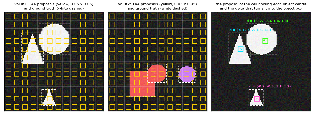
There are three things to read from Figure 10-4.
- Proposal boxes are much smaller than objects. One yellow box is 4.8 pixels, while the shapes are tens of pixels. A proposal box is closer to a placeholder saying "somewhere around here"; the size has to be produced by the head through the delta.
- The deltas in the right panel are not model outputs. They are computed backward from the ground-truth boxes, i.e. the targets the head must hit if that cell is selected. Which cells a trained model actually selects is shown in chapter 11.
- The target deltas are of uniform magnitude. \(\delta_w, \delta_h\) range from 1.1 to 1.8. Since \(e^{1.8} \approx 6\), this means "enlarge 0.05 about 6 times". \(\delta_x, \delta_y\) lie between \(-0.7\) and \(-0.1\). If the object's center is inside the cell, the center offset is at most half a cell, so \(|\delta_x| \le \tfrac{1}{2} \cdot \tfrac{1}{12} \div 0.05 = 0.833\) in the mini model and at most \(\tfrac{1}{2} \cdot \tfrac{1}{24} \div 0.05 = 0.417\) in Nano.
- Proposals at edge cells are discarded — only for large grids
- The official implementation (
gen_encoder_output_proposals) treats a cell as valid only if all four numbers of its proposal box are greater than \(0.01\) and less than \(0.99\), and fills the features and proposals of other cells with 0. The first cell's center is \(0.5 / W\), so edge cells are caught by this when the grid side is 50 or more (\(0.5/50 = 0.01\)). The N–L grids (24–44) have no such cells (\(0.5/44 = 0.0114\)). The mini model does not include this check.
Scoring each cell and picking the top cells
Steps 3 and 4 as formulas: with \(z_j\) the feature of cell \(j\) (output of step 2) and \(s_{j,c}\) the logit of class \(c\) at cell \(j\), the cell score and the selection are
\(s_j = \max_{c}\, s_{j,c}, \qquad \mathcal{T} = \text{the } N \text{ cells with the highest score } s_j\)
This measures "is there likely to be an object of any class in this cell" by the logit of the most confident class. The RF-DETR paper describes this ordering as "the maximum sigmoid of the per-token class logits from the encoder output". Since the sigmoid is monotonically increasing, ranking by the maximum logit or by the value after the sigmoid gives the same order. The code uses the logits directly without a sigmoid.
In Nano, 300 of 576 cells, more than half (52%), are selected. An image does not have 300 objects, so most selected cells are background, and such queries end up with low scores after passing through the decoder. The ratio drops as the grid grows (L: 300 of 1,936 cells, 15%). The mini model selects 12 of 144 cells (8%). If a configuration has fewer cells than queries, the official code selects only as many as there are cells (min(num_queries, number of cells)).
Also keep in mind that the selected cells are ordered by descending score. Query 0 always starts from the highest-scoring cell, and query 299 from the 300th. This ordering later underlies the "use fewer queries" knob.
Boxes of the selected cells and reference boxes
The operation that builds boxes in step 5 is the box reparameterization derived in chapter 9 (bbox_reparam=True). Here is the formula again.
\(\operatorname{reparam}(\delta, r) = \big( \delta_x\, r_w + r_x,\ \ \ \delta_y\, r_h + r_y,\ \ \ e^{\delta_w}\, r_w,\ \ \ e^{\delta_h}\, r_h \big)\)
\(r\) is the starting box and \(\delta\) the delta. The center moves by "some multiple of the starting box's size", and the size is scaled by \(e^{\delta}\). With \(\delta = 0\), the starting box comes out unchanged. RF-DETR uses this operation in three places, two of them inside query selection. With \(j_q\) the index of the \(q\)-th selected cell,
\(\hat{b}^{\text{enc}}_q = \operatorname{reparam}\big( \delta^{\text{enc}}_q,\ b^{\text{grid}}_{j_q} \big), \qquad r_q = \operatorname{reparam}\big( e_q,\ \operatorname{sg}(\hat{b}^{\text{enc}}_q) \big)\)
- \(\delta^{\text{enc}}_q\): the delta obtained by applying
enc_out_bbox_embedto the selected cell's feature \(z_{j_q}\). It depends on the image. - \(\hat{b}^{\text{enc}}_q\): the encoder proposal box. It goes into
enc_outputswith gradients flowing and receives a loss. - \(\operatorname{sg}(\cdot)\): stop-gradient. Only the value is passed on to the decoder side.
- \(e_q\): the \(q\)-th row of
refpoint_embed(four numbers). It is learned independently of the image and initialized to 0. - \(r_q\): the reference box used by the decoder.
The role of refpoint_embed is hard to guess from its name. In the DETR family it was originally a reference point learned per query (the two_stage=False mode of chapter 8 works that way). In the two-stage scheme the reference comes from the image, so this embedding has been repurposed as a learned correction applied to the selected box. \(e_q\) is attached to a rank, not a cell. It is where the model learns values like "the \(q\)-th highest-scoring proposal is generally best shifted this much and enlarged this much". Because it is initialized to 0, \(r_q = \hat{b}^{\text{enc}}_q\) at the start of training.
- Hand calculation — from one cell to a reference box (Nano's cell at row 5, column 7)
- \(b^{\text{grid}} = (0.3125,\ 0.2292,\ 0.05,\ 0.05)\)
- The proposal box computed earlier. Assume this cell is among the top 300.
- An assumed delta output by the box head from this cell's feature (actual values depend on the image and weights).
- Center: multiply the delta by the proposal box's size and add. \(0.4\) means "0.4 times the box width to the right"; the box is 0.05, so the actual shift is \(0.02\).
- Size: scaled by \(e^{\delta}\). In a 384-pixel image, this is a box about 86 pixels wide and 64 pixels tall. This box goes into
pred_boxesofenc_outputs.
- Assume the
refpoint_embedrow for this rank has been trained to these values. Initially it is \((0, 0, 0, 0)\).
- The same operation is applied once more. This time the starting box is \(\operatorname{sg}(\hat{b}^{\text{enc}})\), so the center shift is "0.1 times the encoder proposal's width", and \(e^{-0.1} = 0.9048\). If \(e_q = 0\), then \(r_q = \hat{b}^{\text{enc}}_q\) unchanged.
Note that there is no sigmoid on the boxes. In chapter 8's scheme, values were added in logit space and passed through a sigmoid, so boxes always stayed within 0–1. Reparameterization computes directly in normalized coordinates, so boxes can extend slightly outside the image. The official implementation does not clip them inside the model either.
Content queries do not come from the image
A query entering the decoder has two parts: where it looks (the reference box and the position embedding built from it) and what it holds (a vector updated as it passes through the decoder layers). The initial value of the latter is called the content query.
The natural guess is that the selected cells' features are used as content queries. RF-DETR does not do that. A content query is the \(q\)-th row of the learned embedding query_feat, independent of the image. The selected cell's feature \(z_{j_q}\) is used only up to the box head and enc_outputs and never enters the decoder. That is why, in Figure 10-3, the only arrows going down to the decoder are the reference boxes and query_feat.
| Part of the query | Where it comes from | Depends on the image? | Shape (Nano, inference) |
| Reference box \(r_q\) | The selected cell's encoder proposal box (gradient stopped), adjusted by | Yes | |
| Content query | A row of | No | |
| Query position embedding | Sine embedding of the reference box → | Yes (via the reference box) | |
The LW-DETR paper calls this scheme, in which position comes from the image and content from learned values, "mixed-query selection", and says it follows the DINO paper (the detector by Zhang et al., which only shares its name with the self-distillation DINO of chapter 6). Content queries being independent of the image does not leave them short of information, because the first decoder layer's cross-attention reads features around the reference box. Like refpoint_embed, query_feat is attached to a rank, so query 0's content query is the starting vector of "the query that will handle the highest-scoring proposal". Both embeddings have rows for 13 groups (\(3{,}900\) rows), and only the first 300 rows are used at inference.
Differences from chapter 8's mini implementation
Chapter 8's MiniDeformableDETR(two_stage=True) implemented the same idea. Here are the points where this chapter's MiniRFDETR differs from it. The right column is the official implementation's approach.
| Item | Ch. 8 | This chapter's |
| Proposal → box | \(\sigma(\Delta b + \sigma^{-1}(b^{\text{grid}}))\) — added in logit space | \(\operatorname{reparam}(\delta, b^{\text{grid}})\) — no sigmoid |
| Cells for which box deltas are computed | All cells | Selected cells only (same values, less computation) |
| Selection criterion | Top \(N\) by maximum class logit | Same |
| Query groups | One | \(G\) during training, with separate Linear · layer norm · heads per group |
| | None (the selected box is the reference box) | Applied to the selected box by reparameterization (initialized to 0) |
| Content queries | | Same |
| Query position embedding | Sine embedding of the reference box → 2-layer MLP | Same |
| Reference boxes inside the decoder | Updated every layer (iterative box refinement) | All layers share the initial ones |
| Classification · box heads | Separate per layer | One shared by all layers |
| Features | CNN backbone, 2 levels (12×12, 6×6) | Windowed ViT + projector, 1 level (12×12) |
Decoder layers
This is ⑦ in Figure 10-1. The decoder is a stack of identical layers: 2 in Nano, 3 in the mini model. Each layer takes four inputs.
-
tgt(B, 300, 256): the query vectors. The first layer receives the content queries, and they are updated at each layer. -
query_pos(B, 300, 256): the query position embedding. Every layer receives the same value. - Reference boxes
(B, 300, 1, 4): the 1 in the middle is the level axis (one P4 map). Also the same for every layer. -
memory(B, 576, 256): the projector output.
Three steps in one layer
The order inside a layer is the same post-norm structure as the DETR decoder of chapter 7 and the Deformable DETR decoder of chapter 8. Each step is "compute, add, layer-normalize".
| Step | Operation | Query · key · value | Official settings (measured on Nano) |
| ① Self-attention | | Query · key = | 8 heads ( |
| ② Deformable cross-attention | | 16 heads ( | |
| ③ FFN | Linear → ReLU → Linear | — | 256 → 2048 → 256 |
① is where queries consult each other. This is where they coordinate so that two queries do not take on the same object (chapter 7). During training there are 13 query groups, so, as seen in chapter 9, self-attention runs only within each group: the query axis is split by group, moved onto the batch axis, and then moved back. Groups must not see each other so that using only the first group at inference performs the same computation as during training.
② is the only place where queries look at the image. No position information is added to memory. Deformable attention reads values directly by coordinates, with no dot product against keys, so there is no need to stamp each value with which cell it came from. Having different head counts for self-attention and cross-attention (8 and 16) is a difference from chapter 8's model. The decoder has no dropout (default 0).
ch10_rfdetr_model.py · decoder-layer
class RFDETRDecoderLayer(nn.Module):
    """RF-DETR 디코더 한 층 (post-norm): ① 묶음별 자기 어텐션 → ② 변형 교차 어텐션 → ③ FFN, 각각 뒤에 더하고 층 정규화.

    8장의 DeformableDecoderLayer 와 다른 점: 자기 어텐션과 교차 어텐션의 머리 수가 다르고 (공식 8 · 16),
    학습 때 자기 어텐션을 질의 묶음 안에서만 한다 (Group DETR, 9장 group_self_attention).
    매개변수 이름은 공식 TransformerDecoderLayer 와 같다.
    """

    def __init__(self, dim: int, sa_heads: int, ca_heads: int, ffn_dim: int, n_levels: int, n_points: int):
        super().__init__()
        self.self_attn = nn.MultiheadAttention(dim, sa_heads, batch_first=True)
        self.norm1 = nn.LayerNorm(dim)
        self.cross_attn = MSDeformAttn(dim, n_levels, ca_heads, n_points)
        self.norm2 = nn.LayerNorm(dim)
        self.linear1 = nn.Linear(dim, ffn_dim)
        self.linear2 = nn.Linear(ffn_dim, dim)
        self.norm3 = nn.LayerNorm(dim)

    def forward(self, tgt, query_pos, reference, memory, spatial_shapes, groups: int = 1, return_details=False):
        """tgt · query_pos (B, G·N, D), reference (B, G·N, L, 4) 기준 박스, memory (B, ΣHW, D).

        돌려주는 값: 새 tgt (B, G·N, D).  return_details=True 면 (tgt, 표본점 (B, G·N, M, L, K, 2), 가중치).
        """
        attended = group_self_attention(self.self_attn, tgt + query_pos, tgt, groups)  # ① 같은 묶음끼리만 본다
        tgt = self.norm1(tgt + attended)
        attended, locations, weights = self.cross_attn(tgt + query_pos, reference, memory, spatial_shapes,
                                                       return_details=True)  # ② 기준 박스 안팎의 M·L·K 곳만 읽는다
        tgt = self.norm2(tgt + attended)
        tgt = self.norm3(tgt + self.linear2(F.relu(self.linear1(tgt))))  # ③ FFN
        return (tgt, locations, weights) if return_details else tgt
This is the mini model's decoder layer. group_self_attention from chapter 9 and MSDeformAttn from chapter 8 are reused as they are, and parameter names match the official TransformerDecoderLayer. Applying a shared layer normalization (decoder.norm) once more to each layer's output, not just after the last layer, gives the hs that goes to the heads. The tgt passed to the next layer has not gone through this normalization.
One query reads thirty-two points
Chapter 8 showed that the number of locations one query reads in one cross-attention pass is \(M \cdot L \cdot K\). Plugging in RF-DETR's settings:
- Hand calculation — number of locations read (Nano)
- \(M \cdot L \cdot K = 16 \times 1 \times 2 = 32\)
- 16 heads, 1 level, 2 sampling points per head and level. One query reads 32 locations of the feature map in one layer.
- The number of (query, location) pairs read by 300 queries in one layer.
- With ordinary cross-attention, every query would read all 576 cells.
- One eighteenth as many locations are read. As stressed in chapter 8, this is a ratio of "locations read", not of time. The value projection is still applied to all 576 cells. The linear layer producing offsets has \(2MLK = 64\) outputs, and the one producing weights has \(MLK = 32\) outputs (confirmed in Nano's modules:
Linear(256, 64),Linear(256, 32)).
The fact that the reference is a 4-dimensional box determines where the sampling points go. Dropping the subscript \(l\) from chapter 8's formula since there is only one level, the \(k\)-th sampling point of head \(m\) for query \(q\) is
\(p_{mqk} = (r_x,\ r_y) + \frac{\Delta p_{mqk}}{K} \cdot \frac{(r_w,\ r_h)}{2}\)
\(\Delta p_{mqk}\) is the (2-dimensional) offset produced from the query vector by a linear layer, in units of "\(1/K\) of half the box size". A large box is sampled widely, a small one narrowly. Plug in the reference box from the earlier hand calculation, \(r = (0.3549,\ 0.2192,\ 0.2028,\ 0.1660)\). With the initialization seen in chapter 8, the two sampling points of head 0 start at \(\Delta p = (1, 0)\) and \((2, 0)\).
\(k = 1: \ \Big( 0.3549 + \frac{1}{2} \times \frac{0.2028}{2},\ 0.2192 \Big) = (0.4056,\ 0.2192), \qquad k = 2: \ \Big( 0.3549 + \frac{2}{2} \times \frac{0.2028}{2},\ 0.2192 \Big) = (0.4563,\ 0.2192)\)
The \(k = 2\) point lies on the right edge of the box (\(0.3549 + 0.1014 = 0.4563\)), and the \(k = 1\) point halfway between the center and that edge. The 16 heads split 16 directions among themselves, so at the start of training one query reads 16 points on the border of its reference box and 16 points on a half-size rectangle. As training proceeds, the offsets come to depend on the query's content. These points do not land on cell centers, so values are read by bilinear interpolation. This is what the caption of Figure 2 in the paper means by "the deformable cross-attention layer bilinearly interpolates the projector's output".
Reference boxes are not updated per layer
Chapter 8's Deformable DETR predicted a box at every layer and passed it on as the next layer's reference box (iterative box refinement), so the reference moved closer to the object in deeper layers. RF-DETR's released config sets lite_refpoint_refine=True, in which case all decoder layers share the initial reference box \(r_q\) unchanged. This tutorial calls this lite reference point refinement. The name is a rendering of the config name; the main texts of the LW-DETR and RF-DETR papers do not explain this choice. Only the behavior confirmed in the code is described here.
Original Figure 10-5. How reference boxes are used in a 3-layer decoder. Left: chapter 8's iterative box refinement. Right: RF-DETR's released config. Horizontal arrows are the query vectors passed from layer to layer.
- Left (chapter 8: iterative box refinement): initial reference → layer 1 → box 1. Box 1 follows the dashed line (gradient stop) to become layer 2's reference box and produce box 2, and box 2 becomes layer 3's reference and produces box 3. Box \(d\) is a correction of box \(d-1\).
- Right (RF-DETR: all layers share the initial reference): the reference box \(r\) and the query position embedding are computed once and fed into layers 1, 2 and 3. Only the query vectors pass between layers. Box \(d\) is \(\operatorname{reparam}(\text{delta of layer } d,\ r)\), always starting from \(r\).
| Item | Ch. 8: iterative box refinement | RF-DETR: lite reference point refinement |
| Reference box used by layer \(d\)'s cross-attention | Predicted box of layer \(d - 1\) (gradient stopped) | Always the initial reference box \(r\) |
| Predicted box of layer \(d\) | \(\sigma(\Delta b^{d} + \sigma^{-1}(\operatorname{sg}(\hat{b}^{d-1})))\) | \(\operatorname{reparam}(\delta^{d},\ r)\) |
| Query position embedding | (chapter 8's mini implementation computes it once) | Computed once and shared by all layers |
| Box head | Separate per layer | One shared by all layers |
| What improves in deeper layers | Both the reference box and the query vector | Only the query vector |
In the right-hand scheme, the base of the sampling points (the reference box) does not move in deeper layers. For a deeper layer to look elsewhere it must produce different offsets \(\Delta p\), which it can, since the offsets come from the query vector. The same goes for boxes: each layer answers afresh "how far to shift and how much to enlarge from the initial reference box", with deeper layers simply answering with more refined query vectors. The official code still contains a path that updates the reference per layer when lite_refpoint_refine=False.
The query positional embedding is built from the four numbers of the reference box. Each number is turned into a \(D/2\)-dimensional vector with the sine embedding of chapter 5, the vectors are concatenated, and the result goes into a 2-layer MLP (ref_point_head).
\(\underbrace{(B, 300, 4)}_{\text{reference box}} \ \xrightarrow{\ \text{sine embedding}\ } \ \underbrace{(B, 300, 4 \times 128)}_{= (B, 300, 512)} \ \xrightarrow{\ \texttt{ref\_point\_head}\ } \ \underbrace{(B, 300, 256)}_{\text{query position embedding}}\)
The input and output of ref_point_head measured on Nano are (1, 300, 512) and (1, 300, 256). The mini model takes \(4 \times 64 = 256\) dimensions and outputs 128. This embedding is added to the queries of self-attention and cross-attention (tgt + query_pos), letting each query know "I am responsible for a box of this size at this location".
- A 2D sine positional encoding that is computed but never used
Chapter 7's DETR built a 2D sine positional encoding for each cell of the feature map and added it in the encoder's and decoder's attention. That code survives in RF-DETR's official implementation, which computes a positional encoding of shape (1, 256, 24, 24) on every forward pass and passes it all the way to the decoder. The decoder layers, however, never use it. In fact, replacing this positional encoding with all zeros in Nano and comparing outputs gives a difference of exactly 0.
This is because this configuration has no Transformer encoder and deformable cross-attention reads directly by coordinates. In RF-DETR, two things carry position information: the learned position embedding added to the patch tokens inside the backbone (chapter 6), and, on the query side, the query position embedding built from the reference box. For that reason the mini model does not compute a 2D sine positional encoding at all.
Heads and outputs
This is ⑧ in Figure 10-1. The decoder's output hs has shape (number of layers, B, 300, 256), and applying the two heads to it yields every layer's predictions at once.
Classification head and box head
- Classification head
class_embed: a single linear layer (256 → 91). The outputs are per-class logits, and as since chapter 8, a per-class sigmoid is used with no ∅ slot. The bias follows the prior-probability bias initialization of chapter 4 and is set to \(-\log\frac{1 - 0.01}{0.01} = -\log 99 = -4.595\). Since \(\sigma(-4.595) = 0.01\), at first every query answers "about 1%" for every class. - Box head
bbox_embed: a 3-layer MLP (256 → 256 → 256 → 4, with ReLU in between). The output is not a box but four numbers, a delta \(\delta^{d}_q\). The last layer's weights and bias are initialized to 0.
The two heads are shared by all decoder layers. In chapter 8's iterative box refinement each layer had its own heads, because each layer had a different reference box and "how much to correct" meant something different per layer. In RF-DETR every layer starts from the same reference box, so the same question can be answered by the same head. The heads of two-stage query selection (enc_out_class_embed, enc_out_bbox_embed) are separate layers with the same structure, starting from copies of these two heads, initialization included.
Boxes without a sigmoid
This is the third place box reparameterization is used. With \(h^{d}_q\) the vector for query \(q\) produced by layer \(d\) (an element of hs),
\(\delta^{d}_q = \texttt{bbox\_embed}\big( h^{d}_q \big), \qquad \hat{b}^{d}_q = \operatorname{reparam}\big( \delta^{d}_q,\ r_q \big) = \big( \delta^{d}_{x}\, r_w + r_x,\ \ \delta^{d}_{y}\, r_h + r_y,\ \ e^{\delta^{d}_{w}}\, r_w,\ \ e^{\delta^{d}_{h}}\, r_h \big)\)
(the subscript \(q\) is omitted in the components on the right). The reference box \(r_q\) does not depend on the layer index \(d\); that is lite reference point refinement. Continuing the earlier hand calculation:
- Hand calculation — from reference box to predicted box
- \(r = (0.3549,\ 0.2192,\ 0.2028,\ 0.1660), \qquad \delta^{d} = (-0.05,\ 0.10,\ 0.05,\ -0.02)\)
- The reference box is the value obtained in query selection; the delta is an assumed output of the box head.
- Center: 5% of the reference box's width to the left, and 10% of its height downward.
- Size: width enlarged by 5.1%, height shrunk by 2.0%. The predicted box is \((0.3448,\ 0.2358,\ 0.2132,\ 0.1627)\). When the reference box is already near the object, the decoder's delta only needs to be this small.
Collecting everything initialized to 0 tells you, without computing anything, what the model outputs at the moment training starts.
- Last layer of
enc_out_bbox_embedis 0 → \(\delta^{\text{enc}} = 0\) → \(\hat{b}^{\text{enc}}_q = b^{\text{grid}}_{j_q}\) (the proposal box unchanged) -
refpoint_embedis 0 → \(r_q = \hat{b}^{\text{enc}}_q\) - Last layer of
bbox_embedis 0 → \(\delta^{d} = 0\) → \(\hat{b}^{d}_q = r_q\)
So at first, both the encoder proposals and the predictions of every decoder layer are the proposal boxes of the selected cells (0.05 × 0.05 boxes at cell centers). This was checked on a freshly built mini model.
  초기화 직후의 박스(디코더 3개 층 + 인코더 제안) = 선택된 칸의 제안 박스: 최대 차이 0.00e+00, 박스 크기 0.05 – 0.05
  초기화 직후의 클래스 확률: 평균 0.0157, 범위 0.0043 – 0.0368 (편향 −log 99 = −4.595 → σ = 0.01 근처)
The class probabilities are 0.0043–0.0368 rather than exactly 0.01 because contributions from randomly initialized weights are added to the bias of \(-4.595\). The mean is 0.0157, close to 0.01. Training is the process of learning deltas and logits starting from "small boxes at cell centers with low scores".
The output dict
The model's forward returns a single dict with four entries, using the same names as since chapter 7.
| Name | Contents | Nano, inference (\(B = 1\)) | Mini, inference (\(B = 2\)) | Mini, training (\(B = 2\)) |
| | Class logits of the last decoder layer | | | |
| | Boxes \((c_x, c_y, w, h)\) of the last decoder layer, normalized coordinates | | | |
| | List of | 1 | 2 | 2 |
| | | | | |
- The number of
aux_outputsis (number of decoder layers − 1): 1 for Nano with 2 layers, 2 for the mini model with 3 layers. The auxiliary losses of chapter 7 apply here. - In training mode the query axis is \(G \cdot N\) (mini: \(4 \times 12 = 48\)). Queries are laid out group by group, so in the mini model the first group is queries 0–11, the second 12–23, and so on.
- Nano returns
aux_outputsandenc_outputseven in inference mode (keys of the measured output dict:['aux_outputs', 'enc_outputs', 'pred_boxes', 'pred_logits']). Inference uses only the first two in the table. - The loss applies in the same way to all three kinds of output: the last layer, the earlier layers and the encoder proposals. How it is applied is chapter 11.
Inference post-processing
Building the final list of predictions from the outputs works as in chapter 8. The sigmoid of the logits, (B, 300, 91), is flattened into a single row of query × class with \(300 \times 91 = 27{,}300\) slots, and the top num_select (default 300) by score are picked. Dividing a picked slot's index by 91 gives the query index as the quotient and the class index as the remainder. There is no NMS.
ch10_rfdetr_model.py · postprocess
@torch.no_grad()
def postprocess(outputs, num_select: int | None = None):
    """RF-DETR 의 후처리 = 8장의 postprocess_sigmoid: (질의, 클래스) 쌍의 시그모이드 점수 상위 num_select 개. NMS 없음."""
    return postprocess_sigmoid(outputs, num_select)


def parameter_groups(model: MiniRFDETR):
    """부품별 매개변수 수. 돌려주는 값: [(이름, 전체 수, 추론 때 쓰이는 수)].

    묶음마다 따로 있는 것(enc_output …, 질의 임베딩)은 추론 때 첫 묶음 것만 쓰인다.
    """
    groups = model.group_detr
    rows = [("backbone (WindowedViT)", count_parameters(model.backbone), count_parameters(model.backbone)),
            ("projector (C2f)", count_parameters(model.projector), count_parameters(model.projector))]
    two_stage = sum(count_parameters(m) for m in (model.enc_output, model.enc_output_norm, model.enc_out_class_embed,
                                                   model.enc_out_bbox_embed))
    rows.append(("two-stage heads (x groups)", two_stage, two_stage // groups))
    decoder = sum(count_parameters(m) for m in (model.decoder, model.decoder_norm, model.ref_point_head))
    rows.append(("decoder layers", decoder, decoder))
    heads = count_parameters(model.class_embed) + count_parameters(model.bbox_embed)
    rows.append(("class + box heads", heads, heads))
    queries = count_parameters(model.query_feat) + count_parameters(model.refpoint_embed)
    rows.append(("query embeddings (x groups)", queries, queries // groups))
    return rows
The mini model's postprocess simply calls chapter 8's postprocess_sigmoid (12 out of \(12 \times 3 = 36\) slots). parameter_groups in the same region is the function that builds the parameter table later in this chapter. The official implementation's PostProcess additionally converts boxes into pixel coordinates of the original image. What happens when the score threshold and num_select are changed is shown with the real package in chapter 14.
What changes at inference
The forward pass differs between training and inference in only one place: query groups. At inference only the first \(N\) rows of query_feat and refpoint_embed and the two-stage layers of group 0 are used. On top of that, there are two ways to shrink the architecture after training. They are two of the five knobs the paper uses for NAS, and the paper states that these two are reduced only at inference.
- Use fewer decoder layers. Since the model was trained with a loss on every layer's output, stopping at any layer yields usable predictions. Because the heads are shared and the reference boxes are the same for every layer, running only the first \(d\) layers is the same computation as the output layer \(d\) produced in the full model. Removing all layers (\(d = 0\)) makes the encoder proposals the final output. In that case there is neither self-attention among queries nor cross-attention reading features. The paper likens this state to an NMS-free one-stage detector.
- Use fewer queries. Queries are ordered by descending encoder score, so using only the first \(N'\) discards the lowest-scoring proposals first. This is the scheme described in appendix B of the paper.
Here is the output checking these properties on the mini model (untrained weights, inference mode).
[check] 구조에서 따라 나오는 성질
  추론 출력 = 학습 모드 출력의 첫 묶음 (질의 0 – 11): 최대 차이 0.00e+00
  dec_layers=0 의 출력 = 전체 모델의 enc_outputs: 최대 차이 0.00e+00
  dec_layers=1 의 출력 = 전체 모델의 aux_outputs[0]: 최대 차이 0.00e+00
  dec_layers=2 의 출력 = 전체 모델의 aux_outputs[1]: 최대 차이 0.00e+00
  num_queries=6, dec_layers=0 의 출력 = 인코더 제안 12개의 앞 6개 (점수 순): 최대 차이 0.00e+00
  num_queries=6, 디코더 3층의 로짓 vs 질의 12개일 때의 앞 6개: 최대 차이 2.98e-01 (같지 않다 — 자기 어텐션의 상대가 줄었다)
  선택된 칸은 점수 내림차순으로 놓인다: True
- First check line. The inference output differs by 0 from the first group of the training-mode output (queries 0–11). Because groups do not see each other, removing the other three groups does not change the first group's computation.
- Second to fourth lines. The outputs using only 0, 1 and 2 decoder layers differ by 0 from the full model's
enc_outputs,aux_outputs[0]andaux_outputs[1]. Removing layers does not create a new model; it makes an auxiliary output that was already being produced the final output. - Fifth line. With no decoder and only 6 queries, the output equals the first 6 of the 12 encoder proposals (the top 6 by score).
- Sixth line. With the decoder present, cutting the queries to 6 changes the logits of the remaining 6 compared with 12 queries (max difference 0.298), because the number of peers they consult in self-attention is halved. Unlike the layer count, the query count is not a knob where "what remains stays the same after removal".
- Seventh line. Selected cells are ordered by descending score. This is why "first 6 = top 6 by score" in the fifth line holds.
- In the official implementation these are fixed at construction
- The mini model takes
dec_layersandnum_queriesas arguments toforward, for the experiments in chapter 12. The official implementation has no per-call arguments for these; they are determined by the config at construction time (withdec_layers=0, the encoder proposals are output as predictions, and the query embeddings use the firstnum_queriesrows). The behavior is the same.
Timing with the knobs turned
Keeping the mini model's weights fixed, forward-pass time was measured while changing one knob at a time. Speed does not depend on weight values, so an untrained model was used. These are reference values measured with PyTorch on a laptop GPU and cannot be compared with the paper's latencies (T4, TensorRT).
[손잡이] 같은 가중치, forward 인자만 바꿈 — 추론 모드, 배치 1 과 배치 64 의 순전파 시간
  (40바퀴 가운데 앞 8바퀴를 버린 최솟값)
  설정                                     | 출력 pred_boxes | 배치 1 (ms) | 배치 64 (ms/장)
  기본 (96, 패치 8, 윈도 2, 디코더 3, 질의 12)      | (64, 12, 4)     |        3.03 |      0.135
  디코더 2층                                 | (64, 12, 4)     |        2.68 |      0.130
  디코더 1층                                 | (64, 12, 4)     |        2.30 |      0.123
  디코더 0층                                 | (64, 12, 4)     |        1.64 |      0.112
  질의 6개                                  | (64, 6, 4)      |        3.02 |      0.130
  윈도 1×1 (전부 전역)                         | (64, 12, 4)     |        2.98 |      0.140
  윈도 3×3                                 | (64, 12, 4)     |        3.01 |      0.151
  패치 12 (격자 8×8)                         | (64, 12, 4)     |        3.12 |      0.095
  패치 6 (격자 16×16)                        | (64, 12, 4)     |        3.00 |      0.241
  해상도 64 (격자 8×8)                        | (64, 12, 4)     |        3.08 |      0.088
  해상도 128 (격자 16×16)                     | (64, 12, 4)     |        3.03 |      0.250
- Figure: Figure 10-6 Forward-pass time per image (ms) in the mini RF-DETR when only one knob is changed. Left: batch size 1; right: batch size 64. Blue = default config, orange = number of decoder layers, green = number of queries, pink = number of windows, yellow = patch size, sky blue = resolution. The gray dashed line is the default config's value.
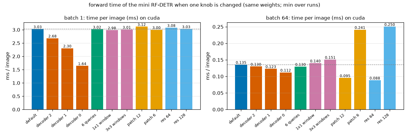
The left and right panels of Figure 10-6 tell completely different stories.
- Batch 1 (left): only the decoder layer count shows. From 3.03 ms, removing one layer at a time brings it down to 2.68, 2.30 and 1.64 ms. The other knobs stay essentially unchanged at 2.98–3.12 ms. The model is so small that time is determined not by the amount of computation but by the number of layer and operation calls. The GPU sits mostly idle.
- Batch 64 (right): the size of the token grid determines the time. An 8×8 grid gives 0.095 and 0.088 ms, 12×12 (default) 0.135 ms, and 16×16 0.241 and 0.250 ms. "Enlarging the patch" and "lowering the resolution" take almost the same time when the grid is the same (patch 12 vs. resolution 64, patch 6 vs. resolution 128). This is the speed-side view of what appendix L of the paper says about accuracy: performance correlates more with the number of spatial positions than with resolution or patch size individually.
- Decoder layers and query count matter little at batch 64. Removing all three decoder layers goes only from 0.135 to 0.112 ms (a 17% reduction). In this mini model the backbone and projector take most of the time.
- More windows did not make it faster. At batch 64: windows 1×1 (all global) 0.140, 2×2 0.135, 3×3 0.151 ms. On a 12×12 grid attention is cheap to begin with (chapter 9), and more windows add one CLS token per window. The differences are within ±10%, and their cause was not investigated separately.
The limits of the measurement should also be noted. When configurations were measured one after another, the same configuration sometimes came out nearly twice as slow from run to run, so all configurations were measured in alternation for 40 rounds and the per-configuration minimum was used. Even so, differences under 0.1 ms at batch 1 or 0.01 ms at batch 64 are best not read into. How these knobs change detection performance is the subject of chapter 12.
Counting parameters
Table 2 of the paper lists RF-DETR Nano at 30.5M parameters. Let us count where this number comes from and how much of it is actually used at inference.
Per-component table
These are the results of splitting the mini model and Nano into the same six components. The right column counts only the first group's share of components that exist once per group.
[매개변수] 부품별
    부품                          |    전체   | 추론 때 쓰이는 것 (묶음 1개)
    backbone (WindowedViT)        |   705,024 |   705,024
    projector (C2f)               |   300,544 |   300,544
    two-stage heads (x groups)    |   202,780 |    50,695
    decoder layers                |   584,096 |   584,096
    class + box heads             |    33,927 |    33,927
    query embeddings (x groups)   |     6,336 |     1,584
    합계                          | 1,832,707 | 1,675,870
    check 표의 합계 = 모델 전체 매개변수 1,832,707: True
  부품별 매개변수 수
    부품                          |      전체     | 추론 때 쓰이는 것 (묶음 1개)
    backbone (windowed DINOv2-S)  |    21,821,184 |    21,821,184
    projector (C2f)               |     1,444,864 |     1,444,864
    two-stage heads (x groups)    |     2,889,939 |       222,303
    decoder layers                |     3,141,312 |     3,141,312
    class + box heads             |       155,999 |       155,999
    query embeddings (x groups)   |     1,014,000 |        78,000
    합계                          |    30,467,298 |    26,863,662
    check 표의 합계 = 모델 전체 매개변수 30,467,298: True
    → 전체 30.47M 은 논문 표 2 의 30.5M 과 맞아떨어진다 (학습용 질의 묶음 13개를 모두 센 수). 추론에 실제로 쓰이는 것은 26.86M.
- Figure: Figure 10-7 Parameter count by component. Left: mini RF-DETR (in thousands); right: RF-DETR Nano (in millions). Blue = total (training), orange hatched = used at inference (one group). Components from the top: backbone, projector, two-stage layers (× groups), decoder layers, classification and box heads, query embeddings (× groups).
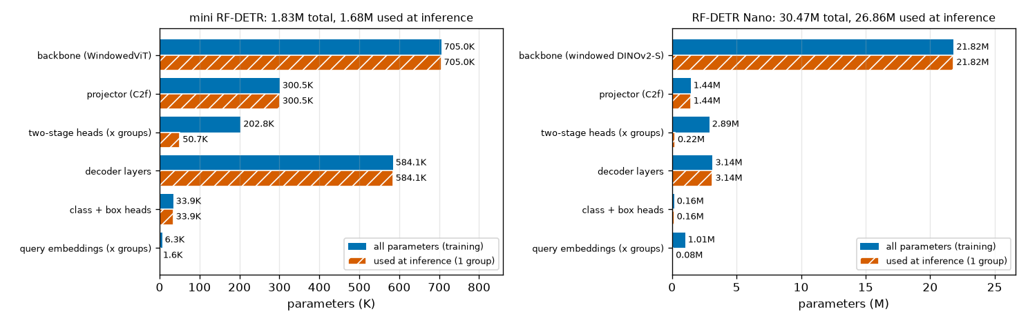
What to read from Figure 10-7 and the tables:
- The backbone dominates. Nano's 21,821,184 are 71.6% of the total. In the mini model the backbone is also the largest (705,024), but its share is 38.5%, meaning the mini model shrank the backbone relatively more.
- Only two components differ between blue and orange: "two-stage heads" and "query embeddings", the components that exist once per group. In Nano, only 300,303 of their combined 3,903,939 are used at inference.
- The decoder has 3.14 million in 2 layers. This row includes the two decoder layers, the shared layer normalization and
ref_point_head. How much one layer accounts for is counted below. - The heads are tiny. The classification and box heads together have 155,999, 0.5% of the total.
Matching the counts by hand
A linear layer has (input dim × output dim) + output dim (bias) parameters. That alone is enough to match several rows of the table. Counting with Nano's numbers (\(D = 256\)):
- Classification head · box head (class + box heads in the table)
- \(\texttt{class\_embed}: \quad 256 \times 91 + 91 = 23{,}296 + 91 = 23{,}387\)
- Linear layer 256 → 91.
- 3-layer MLP: 256 → 256 twice, 256 → 4 once.
- Matches 155,999 in the table.
- Query embeddings (query embeddings in the table)
- \(\texttt{query\_feat}: \quad (13 \times 300) \times 256 = 3{,}900 \times 256 = 998{,}400\)
- 13 groups × 300 queries, 256 dimensions per row.
- Four numbers per row.
- These are 1,014,000 and 78,000 in the table. Only one thirteenth is used at inference.
- Two-stage query selection layers (two-stage heads in the table)
- \(\underbrace{(256 \times 256 + 256)}_{\texttt{enc\_output}} + \underbrace{2 \times 256}_{\texttt{enc\_output\_norm}} + \underbrace{23{,}387}_{\texttt{enc\_out\_class\_embed}} + \underbrace{132{,}612}_{\texttt{enc\_out\_bbox\_embed}}\)
- The four layers of one group. The last two have the same structure as the classification and box heads, so the same counts.
- The count for one group. Matches the "at inference" column of the table.
- Matches 2,889,939 in the table.
- One decoder layer, and the whole decoder (decoder layers in the table)
- \(\text{self-attention}: \quad \underbrace{3 \times (256 \times 256 + 256)}_{\text{query · key · value projections}} + \underbrace{(256 \times 256 + 256)}_{\text{output projection}} = 4 \times 65{,}792 = 263{,}168\)
- Multi-head attention from chapter 5. The number of heads (8) does not affect the parameter count.
- The offset layer has \(2MLK = 64\) outputs and the weight layer \(MLK = 32\). With no key projection, it is smaller than ordinary attention.
- 256 → 2048 → 256. With a hidden dimension 8 times wider, it is the largest component of a layer.
- One decoder layer has about 1.47 million parameters, 71% of them in the FFN.
- Matches 3,141,312 in the table.
ref_point_headis a 2-layer MLP, 512 → 256 → 256.
The backbone can be counted the same way. Plug Nano's numbers (\(C = 384\)) into the formula used to count ViT parameters in chapter 6.
- Backbone (backbone in the table)
- \(\text{one block}: \quad \underbrace{4 \times (384^2 + 384)}_{\text{attention}} + \underbrace{(384 \times 1536 + 1536) + (1536 \times 384 + 384)}_{\text{MLP}} + \underbrace{2 \times 768}_{\text{two layer norms}} + \underbrace{2 \times 384}_{\text{two LayerScales}}\)
- The attention's query, key, value and output projections, the MLP with hidden size 1536, two layer normalizations, and the two per-channel scales (LayerScale) found in DINOv2 blocks.
- Since \(384^2 = 147{,}456\), attention is \(4 \times 147{,}840 = 591{,}360\) and the MLP is \(591{,}360 + 590{,}208 = 1{,}181{,}568\).
- The 16×16 patch convolution, the position embedding \((24^2 + 1) \times 384\), and the CLS token and mask token (the latter was used in pretraining and is not used for detection).
- Matches 21,821,184 in the table. Keep in mind that the size of the position embedding depends on the resolution; this comes up right below.
The projector (1,444,864) was counted earlier. Adding the six rows gives \(21{,}821{,}184 + 1{,}444{,}864 + 2{,}889{,}939 + 3{,}141{,}312 + 155{,}999 + 1{,}014{,}000 = 30{,}467{,}298\). Every parameter of the model has been recounted by hand row by row, and the total does not differ from the real model's by a single parameter.
The paper's 30.5M and the number used at inference
Nano's 30,467,298 total parameters round to 30.5M, matching Table 2 of the paper. This number, however, includes parameters used only during training: the share of the last 12 of the 13 query groups.
\(\underbrace{12 \times 222{,}303}_{\text{two-stage layers}} + \underbrace{12 \times 78{,}000}_{\text{query embeddings}} = 2{,}667{,}636 + 936{,}000 = 3{,}603{,}636\)
That is 11.8% of the total. Subtracting it, the parameters actually used at inference number \(30{,}467{,}298 - 3{,}603{,}636 = 26{,}863{,}662\) (26.9M). In the mini model, 156,837 of 1,832,707 (8.6%) are unused at inference.
The paper does not say how it counted parameters. What can be confirmed is only that "the total parameter count of the released Nano model matches the paper's 30.5M". When comparing parameter counts with other detectors, it is enough to know that such differences can exist. Strictly speaking, a little more is unused at inference (the backbone's 384-parameter mask token, and, if the auxiliary outputs and enc_outputs are not used, the computation done only for them).
The size family
RF-DETR is not a single model but a family of sizes. The table reproduces the COCO detection configurations from Table 7 of the paper, with parameter counts and performance added (Table 2 and appendix Table 12 of the paper).
| Size | Backbone | Resolution | Patch | Windows (per side) | Decoder layers | Queries | Parameters (paper) | GFLOPs | Latency (ms) | COCO AP |
| N | DINOv2-S | 384 | 16 | 2 | 2 | 300 | 30.5M | 31.9 | 2.3 | 48.0 |
| S | DINOv2-S | 512 | 16 | 2 | 3 | 300 | 32.1M | 59.8 | 3.5 | 52.9 |
| M | DINOv2-S | 576 | 16 | 2 | 4 | 300 | 33.7M | 78.8 | 4.4 | 54.7 |
| L | DINOv2-S | 704 | 16 | 2 | 4 | 300 | 33.9M | 125.6 | 6.8 | 56.5 |
| XL | DINOv2-B | 700 | 20 | 1 | 5 | 300 | 126.4M | 299.3 | 11.5 | 58.6 |
| 2XL | DINOv2-B | 880 | 20 | 2 | 5 | 300 | 126.9M | 438.4 | 17.2 | 60.1 |
N, S, M and L use the same backbone (DINOv2-S, 12 blocks, dimension 384), the same projector and the same hidden_dim. Among the architecture-defining values in the released configs, the four sizes differ only in resolution, number of decoder layers and position embedding grid. XL and 2XL switch the backbone to DINOv2-B and use patch size 20 (Table 7 of the paper). What stands out in the table is that from N to L the GFLOPs quadruple, from 31.9 to 125.6, while the parameters barely change, from 30.5M to 33.9M. Let us confirm why with numbers.
- From N to S, M and L — the added parameters
- \(\text{one decoder layer} = 1{,}471{,}840, \qquad \text{position embedding} = (g^2 + 1) \times 384\)
- These are the only two components that vary with size. A higher resolution means more tokens, but the weights of the layers processing them do not depend on the token count. Only the position embedding grows to fit the \(g \times g\) grid.
- At resolution 512 the grid is \(g = 32\). Matches the paper's 32.1M.
- Resolution 576, \(g = 36\). The paper's 33.7M.
- Resolution 704, \(g = 44\). The paper's 33.9M. M and L have the same number of decoder layers, so they differ only by 246K position embedding parameters.
The three hand-computed values exactly matched the counts (32,111,170 · 33,687,458 · 33,933,218) obtained by building Small, Medium and Large models without weights from the configs of the installed package (rfdetr 1.12.1). The parameter count is a model's "memory capacity", while GFLOPs and latency are "amount of work". Processing more tokens with the same weights increases only the amount of work. RF-DETR's size family scales mainly through token count and decoder depth, which is why it can be obtained all at once with weight-sharing NAS (chapter 12). The 0.5M difference between XL and 2XL also checks out the same way: both have 5 decoder layers, and the position embeddings differ by \((44^2 - 35^2) \times 768 = 546{,}048\) (DINOv2-B has dimension 768; these two models could not be built in this environment, so only the arithmetic against the paper's numbers was checked).
Walking through the mini RF-DETR
MiniRFDETR in code/ch10_rfdetr_model.py packs everything in this chapter into a little over 200 lines. Only the decoder layer and the assembly code are new; the components come from the files of earlier chapters.
-
ch07_detr.py:MLP,sine_embed(sine embedding of coordinates) -
ch08_deformable.py:MSDeformAttn,gen_proposals(proposal box grid),postprocess_sigmoid -
ch09_lwdetr_parts.py:WindowedViT,MultiScaleProjector,box_reparam,group_self_attention
Configuration
ch10_rfdetr_model.py · config
DEFAULT_CONFIG = {
    "num_classes": NUM_CLASSES,  # 3 (원 · 사각형 · 삼각형)
    "num_queries": 12,           # 묶음 하나의 질의 수 (공식 300)
    "group_detr": 4,             # 학습 때의 질의 묶음 수 (공식 13). 추론 때는 첫 묶음만 쓴다
    "hidden_dim": 128,           # 프로젝터 출력 · 디코더의 차원 (공식 256)
    "dec_layers": 3,             # 디코더 층 수 (Nano 2, Small 3, Medium 4)
    "sa_heads": 8,               # 디코더 자기 어텐션의 머리 수 (공식 8)
    "ca_heads": 16,              # 디코더 변형 교차 어텐션의 머리 수 (공식 16)
    "dec_n_points": 2,           # 머리 · 레벨마다의 표본점 수 (공식 2)
    "ffn_dim": 256,              # 디코더 FFN 의 은닉 차원 (공식 2048)
    "img_size": 96,              # 기본 입력 해상도 (Nano 384)
    "patch_size": 8,             # 기본 패치 크기 (Nano 16) → 토큰 격자 12×12 (Nano 24×24)
    "vit_dim": 96,               # 백본의 차원 (DINOv2-S 384)
    "vit_depth": 6,              # 백본의 블록 수 (DINOv2-S 12)
    "vit_heads": 4,              # 백본의 머리 수 (DINOv2-S 6)
    "out_feature_indexes": (2, 4, 6),  # 특징을 꺼내는 층 (Nano [3, 6, 9, 12]) → 윈도 블록 0, 1, 3, 5 / 전역 블록 2, 4
    "num_windows": 2,            # 한 변의 윈도 수 (Nano 2)
    "projector_scale": ("P4",),  # 프로젝터가 만드는 스케일 (공식 ["P4"])
}
The comment on each line gives the official value. Names were kept as close to the official config as possible. A model can be built by overriding only some values, as in MiniRFDETR(group_detr=1), which is how the code for chapters 11–13 uses it.
Model
ch10_rfdetr_model.py · model — a long code listing collapsed in the original, so it is not reproduced here. It is in the model region of code/ch10_rfdetr_model.py.
Read forward against the numbers in Figure 10-1.
- ①–⑤
extract_features. The backbone produces three feature maps and the projector one P4 map.flatten(2).transpose(1, 2)flattens(B, 128, 12, 12)intomemory(B, 144, 128). - ⑥
select_queries. A loop runs once per group.all_logits.max(-1).values.topk(num_queries)is "the top \(N\) cells by maximum class logit", andbox_reparam(delta, proposals[top])gives the encoder proposal boxes. The official implementation applies layer normalization to the features of the selected cells, while this code applies it to all cells and then selects; since layer normalization is computed per token, the result is the same. - Reference boxes and queries. The single line
box_reparam(self.refpoint_embed.weight[:total][None], enc_boxes.detach())is \(r_q = \operatorname{reparam}(e_q, \operatorname{sg}(\hat{b}^{\text{enc}}_q))\).query_posis computed only once, outside the loop.tgtisquery_featexpanded to the batch size. - ⑦ Decoder. Only
tgtchanges inside the loop. The samequery_posandreference_inputgo into every layer.decoder_norm(tgt)from each layer is collected intohs. - ⑧ Heads.
self.class_embed(hs)andbox_reparam(self.bbox_embed(hs), reference)produce every layer's predictions at once. The last layer givespred_*, the restaux_outputs.
The num_layers == 0 branch is the "all decoder layers removed" case: it returns the query selection results directly as pred_logits and pred_boxes and stops. The initialization in __init__ also follows the official implementation: classification bias \(-\log 99\), last layer of the box head 0, refpoint_embed 0, and the two-stage heads starting as copies of the decoder heads.
Running it and tracing shapes
Running the script first prints the mini model's config (identical to DEFAULT_CONFIG above, so omitted here) and the shapes at each step. This is the result for two validation images from the shape world (\(B = 2\)).
  윈도 블록 [0, 1, 3, 5], 전역 블록 [2, 4]
[모양 추적] 입력 (2, 3, 96, 96) — 추론 모드 (묶음 1개)
    그림                                     (2, 3, 96, 96)
    패치 임베딩 + CLS + 위치 임베딩                  (2, 145, 96)
    윈도 우선 재배열 + 윈도마다 CLS                   (8, 37, 96)
    백본 특징 맵 × 3 (층 [2, 4, 6])              (2, 96, 12, 12)
    프로젝터 출력 (P4)                           (2, 128, 12, 12)
    memory (칸을 한 줄로)                       (2, 144, 128)
    제안 박스 (칸마다 하나)                         (144, 4)
    칸마다의 클래스 로짓                            (2, 144, 3)
    선택된 칸 번호 topk                          (2, 12)
    인코더 제안: 로짓 / 박스                        ((2, 12, 3), (2, 12, 4))
    기준 박스 (모든 층 공유)                        (2, 12, 4)
    기준 박스의 사인 임베딩 → ref_point_head         ((2, 12, 256), (2, 12, 128))
    디코더 층별 질의 임베딩 hs                       (3, 2, 12, 128)
    pred_logits / pred_boxes               ((2, 12, 3), (2, 12, 4))
    aux_outputs                            2개 (앞 층들), 각각 같은 모양
    (참고) 2차원 사인 위치 인코딩          (144, 128) — 공식 구현은 이것을 계산해 디코더에 넘기지만 디코더가 쓰지 않는다 (아래 Nano 대조에서 확인)
  학습 모드 (묶음 4개): pred_logits (2, 48, 3), enc_outputs (2, 48, 3), hs (3, 2, 48, 128)
This output is the bottom line (lighter text) of Figure 10-1. A few lines are worth pointing out. Right after embedding, (2, 145, 96) is 1 CLS + 144 patches; rearranging window-major and prepending a CLS to each window gives (8, 37, 96) (\(8 = 2 \times 4\), \(37 = 36 + 1\)). The sine embedding of the reference boxes is \(4 \times 64 = 256\)-dimensional, and ref_point_head turns it into 128 dimensions. In training mode the query axis becomes \(4 \times 12 = 48\).
Next come Nano's shapes, read from actual inputs and outputs with hooks on every module.
[RF-DETR Nano 대조] rfdetr 1.12.1, 가중치 rf-detr-nano.pth, 장치 cpu
  설정: resolution 384, patch_size 16, num_windows 2, out_feature_indexes [3, 6, 9, 12], hidden_dim 256, dec_layers 2, num_queries 300, group_detr 13, sa_nheads 8, ca_nheads 16, dec_n_points 2, projector_scale ['P4']
  백본: 차원 384, 블록 12, 머리 6, 윈도 블록 [0, 1, 2, 4, 5, 7, 8, 10, 11], 레지스터 토큰 0
  단계별 텐서 모양 (추론 모드, 배치 1, 훅으로 실제로 잰 값)
    그림                                           (1, 3, 384, 384)
    임베딩 출력 (윈도 우선 + 윈도마다 CLS)                    (4, 145, 384)
    윈도 블록의 어텐션 입력 (예: 블록 0)                      (4, 145, 384)
    전역 블록의 어텐션 입력 (블록 [3, 6, 9])                 (1, 580, 384)
    백본 특징 맵 × 4                                  (1, 384, 24, 24)
    프로젝터 출력                                      (1, 256, 24, 24)
    2차원 사인 위치 인코딩                                (1, 256, 24, 24)
    enc_output (모든 칸)                            (1, 576, 256)
    칸마다의 클래스 로짓 (순위를 매길 때)                       (1, 576, 91)
    선택된 칸의 클래스 로짓 (enc_outputs)                  (1, 300, 91)
    선택된 칸의 박스 델타                                 (1, 300, 4)
    ref_point_head 입력 → 출력                       ((1, 300, 512), (1, 300, 256))
    변형 교차 어텐션 입력: 질의 / 기준 박스 / memory            ((1, 300, 256), (1, 300, 1, 4), (1, 576, 256))
    디코더 층 출력 × 2                                 (1, 300, 256)
    class_embed 출력 (층 축 포함)                      (2, 1, 300, 91)
    pred_logits / pred_boxes                     ((1, 300, 91), (1, 300, 4))
    → 패치 토큰 24×24 = 576개, 윈도 2×2 로 나누면 윈도마다 144개 + CLS 1개. 전역 블록은 [3, 6, 9] (0 부터 센 번호)
    → 특징을 꺼내는 자리: 블록 [2, 5, 8, 11] 의 출력 (out_feature_indexes [3, 6, 9, 12] 는 '블록 몇 개를 지난 뒤' 라는 뜻)
    → 출력 키: ['aux_outputs', 'enc_outputs', 'pred_boxes', 'pred_logits']  (추론 모드에서도 aux_outputs · enc_outputs 가 나온다)
This output is the top line of Figure 10-1. "Per-cell class logits" appear twice, once with 576 cells and once with 300, because the official implementation calls the same linear layer twice in one forward pass (once to rank all cells, once to build enc_outputs for the selected cells). The mini model computes it once and selects from the result. The reference box shape (1, 300, 1, 4) in deformable cross-attention shows there is one level, and the class_embed output (2, 1, 300, 91) shows that the head is applied at once to the whole of hs, layer axis (2) included.
Comparison with the official implementation
The claim that "the architecture and computation are the same as the official implementation" was checked numerically. The weights of everything after the projector in MiniRFDETR (two-stage query selection, decoder, heads) were copied directly into the official Transformer and LWDETR classes, the same images were fed in, and the outputs were compared. Weights that are initialized to 0 were perturbed with random values before copying so that every path took part in the computation. This was a one-off comparison not included in the tutorial code (the backbone and projector comparison is in chapter 9).
| Comparison | Maximum output difference |
| P4, training mode (4 groups): | 1.43e-06 (auxiliary outputs 1.43e-06, |
| P4, inference mode: | 9.54e-07 (auxiliary outputs 9.54e-07, |
| P3 · P4 · P5 (3 levels), training / inference | 1.91e-06 / 1.43e-06 |
These were measured on inputs where the mean absolute logit is 4.7, so the differences are at the level of 32-bit floating-point rounding. In other words, transferring the weights produces the same output. There are also places where the mini model does things differently from the official implementation. All differences other than size are listed below.
| Item | Mini RF-DETR | Official implementation | Effect |
| 2D sine positional encoding | Not computed | Computed and passed on, but unused by the decoder | None (output difference 0 on Nano) |
| Validity range check on proposal boxes | None | Cells outside 0.01–0.99 are discarded | None if the grid side is under 50 |
| Coordinate order in the sine embedding | \((x, y, w, h)\) | \((y, x, w, h)\) | Only the column order of the MLP input differs; swapping the first layer's columns when transferring weights makes them match |
| | Arguments to | Config at model construction | Same behavior |
| Padding mask · valid ratios | None | Present | None if all images are the same size |
| Input normalization | | ImageNet mean and standard deviation, outside the model | Difference in preprocessing |
| Changing patch size per call | Possible (patch embedding weights are interpolated) | Fixed at construction | For the experiments in chapter 12 |
| Segmentation head · keypoints · mixed precision | None | Available as options | Segmentation head in chapter 13 |
| Backbone weights | Start from random initialization | DINOv2 pretrained weights | Covered in chapter 11 |
Multi-scale is also possible. MiniRFDETR(projector_scale=("P3", "P4", "P5")) uses three levels (24×24, 12×12, 6×6); only its forward-pass shapes and numerical agreement with the official implementation were checked. It was not trained.
[다중 스케일] projector_scale = (P3, P4, P5): spatial_shapes [(24, 24), (12, 12), (6, 6)], memory (2, 756, 128), pred_boxes (2, 12, 4), 매개변수 2,794,515개
Summary
- The RF-DETR forward pass is patch embedding → DINOv2 ViT with windows → several feature maps → projector (P4) → two-stage query selection → decoder → shared heads. For Nano (384×384): 576 tokens, feature maps
(B, 384, 24, 24)× 4, projector output(B, 256, 24, 24), outputs(B, 300, 91)and(B, 300, 4). - What changed from LW-DETR: the backbone (CAEv2 → DINOv2), projector normalization (batch → layer), the placement of windowed blocks, the segmentation head, and NAS. Layer normalization is computed within one image, so gradient accumulation gives the same gradient as a large batch.
-
num_windowsis the number of windows per side, \(W_n\). The input side length must be a multiple of \(p \cdot W_n\) (a multiple of 32 for Nano). - The CLS token is copied into every window. Windowed blocks see \((B W_n^2,\ n + 1,\ C)\) and global blocks only change the view to \((B,\ W_n^2(n + 1),\ C)\). Nano:
(4B, 145, 384)↔(B, 580, 384). - The windowed blocks are {0, 1, 3, 4, 6, 7, 9, 10} according to appendix A of the paper, but in the released code's actual behavior they are the complement of
out_feature_indexes=[3, 6, 9, 12], {0, 1, 2, 4, 5, 7, 8, 10, 11} (global: 3, 6, 9). - The projector concatenates the four feature maps along channels (1536) and produces 256 channels with C2f and layer normalization. It does not change the resolution.
- Two-stage query selection: proposal boxes for every cell (cell center, 0.05) → per-group Linear + layer normalization → top \(N\) cells by maximum class logit → those cells' deltas give \(\hat{b}^{\text{enc}} = \operatorname{reparam}(\delta^{\text{enc}}, b^{\text{grid}})\). These predictions receive a loss through
enc_outputs. - The reference box is \(r_q = \operatorname{reparam}(e_q, \operatorname{sg}(\hat{b}^{\text{enc}}_q))\), and the content query is
query_feat, independent of the image.refpoint_embed\(e_q\) is a rank-attached correction that starts at 0. - A decoder layer is per-group self-attention (8 heads) → deformable cross-attention (16 heads · 1 level · 2 sampling points, 32 locations per query) → FFN (2048). All layers use the same reference boxes, the same query position embedding and the same heads.
- Boxes are produced without a sigmoid as \(\hat{b}^{d}_q = \operatorname{reparam}(\delta^{d}_q, r_q)\). Because of zero initialization, every output is initially the proposal box of the selected cell.
- At inference only the first group is used. Using only the first few decoder layers gives the same output as those layers' auxiliary outputs, and with 0 layers the encoder proposals are the output. Reducing the queries also changes the outputs of the remaining queries.
- Nano has 30,467,298 parameters (paper: 30.5M), of which 26,863,662 are used at inference. N → L share the same backbone, so only decoder layers (1,471,840 per layer) and the position embedding grow.
You now know what one RF-DETR model looks like. An image becomes 576 tokens, is refined while alternating between windowed and global attention, passes through the projector to become the feature map that 300 queries read, and the queries start from boxes selected from the image and produce answers in just two layers. The mini model in this chapter, however, has never been trained. Right after initialization, its output was nothing but 12 boxes of 0.05 × 0.05 and scores of a little over 1%. Chapter 11 actually trains this architecture: per-group Hungarian matching and the IA-BCE loss on every layer and on the encoder proposals, layer-wise learning rates for the backbone, and EMA weight averaging. It also uses the shape world to check what the paper's "scheduler-free" training setup is and how big a difference pretraining makes.
Exercises
- Exercise 1 · Token counts and shapes
- RF-DETR Small has resolution 512, patch size 16 and
num_windows=2, with the same backbone as Nano (dimension 384). For one image (\(B = 1\)), find (a) the number of patch tokens, (b) the tensor shape in a windowed block, (c) the tensor shape in a global block, and (d) the shape of one feature map output by the backbone. - Answer. (a) \(g = 512 / 16 = 32\), so \(32^2 = 1{,}024\).
- (b) There are \(2 \times 2 = 4\) windows, each with \(n = (32/2)^2 = 256\) patch tokens. Adding the CLS gives 257, so
(4, 257, 384). - (c) \(4 \times 257 = 1{,}028\), so
(1, 1028, 384). That is 3 more tokens than without windows (\(1{,}024 + 1 = 1{,}025\)). - (d) Removing the CLS and restoring the grid gives
(1, 384, 32, 32). There are four of these. - Exercise 2 · The divisibility constraint
- (a) Can a 600×600 image be fed to a model with patch size 16 and
num_windows=2? If not, find the two valid resolutions closest to 600. (b) With patch size 20 andnum_windows=2, is 600×600 valid? If so, find the number of tokens. - Answer. (a) The side must be a multiple of \(p \cdot W_n = 32\). \(600 / 32 = 18.75\), so it cannot. The nearest multiples are \(32 \times 18 = 576\) and \(32 \times 19 = 608\).
- (b) \(p \cdot W_n = 40\) and \(600 / 40 = 15\), so it is valid. The grid is \(600 / 20 = 30\), giving \(900\) tokens, with \(15 \times 15 = 225\) per window.
- Exercise 3 · Determining the windowed blocks
- Apply the released code's rule ("from the numbers 0 through the last value of
out_feature_indexes, removeout_feature_indexes") to (a)[2, 5, 8, 11]and (b) the mini model's(2, 4, 6), and find the windowed and global blocks. There are 12 and 6 blocks respectively. (c) In (b), how many global blocks has the first extracted feature gone through? - Answer. (a) \(\{0, \dots, 11\} \setminus \{2, 5, 8, 11\} = \{0, 1, 3, 4, 6, 7, 9, 10\}\) are the windowed blocks, and the global blocks are \(\{2, 5, 8, 11\}\). This is the same set as stated in appendix A of the paper.
- (b) \(\{0, \dots, 6\} \setminus \{2, 4, 6\} = \{0, 1, 3, 5\}\) are the windowed blocks (6 is not a block number), and the global blocks are \(\{2, 4\}\). This matches "windowed blocks [0, 1, 3, 5], global blocks [2, 4]" in the log.
- (c) None. The 2 in
out_feature_indexesmeans "after 2 blocks", i.e. the output of blocks 0 and 1, both windowed. The second feature (after blocks 0–3) has gone through global block 2 once, and the third feature twice. - Exercise 4 · From proposal box to encoder proposal box
- In RF-DETR Small (32×32 grid, resolution 512), the cell at (row 10, column 20) was selected and the box head output \(\delta^{\text{enc}} = (-0.5,\ 0.2,\ \log 4,\ \log 2)\). Find (a) this cell's proposal box, (b) the encoder proposal box, and (c) that box's size in pixels. (d) If
refpoint_embedis still 0, what is the reference box? - Answer. (a) \(\big( \tfrac{20.5}{32},\ \tfrac{10.5}{32},\ 0.05,\ 0.05 \big) = (0.6406,\ 0.3281,\ 0.05,\ 0.05)\).
- (b) \(c_x = -0.5 \times 0.05 + 0.6406 = 0.6156\), \(c_y = 0.2 \times 0.05 + 0.3281 = 0.3381\), \(w = e^{\log 4} \times 0.05 = 0.2\), \(h = e^{\log 2} \times 0.05 = 0.1\). The box is \((0.6156,\ 0.3381,\ 0.2,\ 0.1)\).
- (c) \(0.2 \times 512 = 102.4\) pixels and \(0.1 \times 512 = 51.2\) pixels.
- (d) \(\operatorname{reparam}(0, \hat{b}^{\text{enc}}) = \hat{b}^{\text{enc}}\), so it is the box from (b) unchanged (only the gradient is cut).
- Exercise 5 · Counting the mini model's parameters
- The mini RF-DETR has \(D = 128\), 3 classes, and 12 queries × 4 groups. Find (a) the combined parameter count of the classification and box heads, (b) the total and inference-time counts of the query embeddings (
query_feat+refpoint_embed), and (c) the count of the two-stage query selection layers for one group and for four groups, and check them against the log. - Answer. (a) Classification head \(128 \times 3 + 3 = 387\). Box head \(2 \times (128 \times 128 + 128) + (128 \times 4 + 4) = 2 \times 16{,}512 + 516 = 33{,}540\). Total \(33{,}927\) (class + box heads in the log).
- (b) \(48 \times 128 + 48 \times 4 = 6{,}144 + 192 = 6{,}336\). At inference, \(12 \times 132 = 1{,}584\).
- (c) One group: \((128 \times 128 + 128) + 2 \times 128 + 387 + 33{,}540 = 16{,}512 + 256 + 387 + 33{,}540 = 50{,}695\). Four groups: \(4 \times 50{,}695 = 202{,}780\).
- Exercise 6 · One more decoder layer
- One Nano decoder layer has 1,471,840 parameters. (a) If the FFN hidden dimension is reduced from 2048 to 1024, how many does one layer have? (b) If only the decoder in Nano's config is increased from 2 to 6 layers (resolution still 384), how many parameters does the whole model have? (c) If the cross-attention sampling points are increased from 2 to 4, by how much does one layer's parameter count grow?
- Answer. (a) The FFN becomes \((256 \times 1024 + 1024) + (1024 \times 256 + 256) = 263{,}168 + 262{,}400 = 525{,}568\). It was \(1{,}050{,}880\), so it shrinks by \(525{,}312\), giving \(1{,}471{,}840 - 525{,}312 = 946{,}528\).
- (b) \(30{,}467{,}298 + 4 \times 1{,}471{,}840 = 30{,}467{,}298 + 5{,}887{,}360 = 36{,}354{,}658\). The resolution is the same, so the position embedding is unchanged.
- (c) The offset layer's output becomes \(2 \times 16 \times 1 \times 4 = 128\) and the weight layer's output \(64\). \((256 \times 128 + 128) + (256 \times 64 + 64) = 32{,}896 + 16{,}448 = 49{,}344\), versus the original \(16{,}448 + 8{,}224 = 24{,}672\), an increase of \(24{,}672\). Adding sampling points is very cheap in parameters.
- Exercise 7 · What can and cannot be removed
- For a trained RF-DETR: (a) The output of a model with the last decoder layer removed equals which output of the original model? Why exactly the same? (b) Is the output of a model with queries reduced from 300 to 100 the same as the outputs of the first 100 queries of the original model? Explain. (c) Would the answer to (a) change for a model using iterative box refinement (chapter 8)?
- Answer. (a) It equals the original model's last auxiliary output (
aux_outputs[-1]). Computation in the decoder flows only from earlier to later layers, so removing a later layer does not change the earlier layers' computation. Since the heads are shared by all layers and the reference boxes are the same for every layer, applying the heads to an earlier layer's output is exactly the computation by which the original model produced its auxiliary output. The difference was 0 in the mini model's check. - (b) No. In the decoder's self-attention, each query consults all other queries in its group. When 200 queries disappear, the peers the remaining 100 consult change, so their outputs change (max logit difference 0.298 in the mini model). With 0 decoder layers, however, there is no self-attention, so the output is then exactly the first 100 encoder proposals.
- (c) The answer stays the same. With iterative box refinement too, layer \(d\)'s output depends only on the computation up to layer \(d\), so removing later layers leaves the earlier layers' auxiliary outputs intact. The only difference is that each layer has its own heads, and the heads of removed layers are simply discarded along with them. Either way, the required condition is that "the model was trained with a loss on every layer's output".
See also
Favorite site
- 10. RF-DETR Architecture
- code/ch10_rfdetr_model.py
- RF-DETR: Neural Architecture Search for Real-Time Detection Transformers (arXiv:2511.09554)
- LW-DETR: A Transformer Replacement to YOLO for Real-Time Detection (arXiv:2406.03459)
- DINOv2: Learning Robust Visual Features without Supervision (arXiv:2304.07193)
- Github - roboflow/rf-detr