RF-DETR:Tutorial:09-RT-DETR-LW-DETR
lastmod 2026-11-18created 2026-11-185 edits
Real-time DETR: RT-DETR and LW-DETR is chapter 9 of the RF-DETR tutorial. The DETR family through chapter 8 was accurate and clean, but slow. This chapter looks at the two models that brought that lineage into real time. RT-DETR (Zhao et al., 2023) is covered only at the level of ideas, while LW-DETR (Chen et al., 2024), the direct foundation of RF-DETR, is taken apart piece by piece and worked through with equations, hand calculations, and code. The pieces are window attention and window-major organization, the C2f projector, the IoU-aware BCE loss, Group DETR, and box reparameterization. Every ingredient used to assemble RF-DETR in chapter 10 comes from here.
- Original: 09. Real-time DETR: RT-DETR and LW-DETR (reading time about 110 minutes per the original, difficulty ★★★★☆)
- Practice code:
code/ch09_lwdetr_parts.py. It does no training. For each part (window attention · window-major organization · C2f projector · IA-BCE loss · Group DETR · box reparameterization) it prints a hand-calculated example, checks the values against PyTorch built-in operations, and draws five figures. It takes about 32 seconds on a laptop GPU, and about 7 seconds on CPU with--quick. The mini RF-DETR in chapter 10 reuses the parts in this file as they are. - Previous: 08. Deformable DETR: Looking Only Where Needed / Next: 10. The Architecture of RF-DETR
What this chapter covers
- Why the DETR family could not reach real time, and why the NMS time of the YOLO family matters in comparisons
- The three ideas RT-DETR introduced (hybrid encoder, query selection, adjusting the number of decoder layers), to the extent the paper describes them
- The overall structure of LW-DETR: ViT encoder → projector → shallow decoder, and its five sizes
- Deriving the operation count of window attention, and confirming by experiment why global layers must be interleaved
- Window-major organization: why laying out tokens window by window makes the reordering disappear, following the paper's 4×4 example by hand
- Multi-level feature aggregation and the C2f projector: counting channels and parameters by hand
- IoU-aware BCE loss (IA-BCE): the paper's equation, how it maps to the official implementation, and the derivation and hand calculation of the fixed point where "the score is pulled toward the IoU"
- Group DETR: how copying the queries into groups adds supervision signal, and why the groups are kept from seeing each other
- Box reparameterization: how it differs from the logit-space addition of chapter 8, and why the same delta means the same thing regardless of box size
- Telling apart the numbers the papers report and the numbers this tutorial measured (some results were not reproduced in this chapter's measurements)
- Notation in this chapter
-
- \(N\): the number of tokens (patches) the encoder handles (same as in chapter 5 · chapter 6). In chapters 7 · 8, \(N\) was the number of object queries, but in this chapter the number of queries is written \(N_q\). The docstrings in the code write the number of queries as
N((B, G·N, D)). - \(W_n\): the number of windows per side. The token grid is divided into \(W_n\) parts horizontally and \(W_n\) parts vertically, giving \(W_n^2\) windows. This is
num_windowsin the code andW_nin the logs. When the LW-DETR paper says "16 windows", \(W_n = 4\). - \(p\): the classification score after the sigmoid (the notation of chapter 4). The LW-DETR paper writes it as \(s\). \(z\) is the logit, \(t\) the classification target, and \(u\) the IoU between the predicted box and the ground-truth box.
- \(\alpha\): in this chapter, the exponent of IA-BCE (\(t = p^{\alpha} u^{1-\alpha}\), value 0.25). It has the same letter and the same value as the balancing weight \(\alpha\) of the focal loss in chapter 4, but it is a different thing. When the focal loss one is meant, it is written explicitly as "the focal loss \(\alpha\)". \(\gamma\) is the exponent of the modulating factor in both losses (value 2).
- \(G\): the number of query groups (\(K\) in the Group DETR paper). \(T\): the number of ground-truth objects in one image (chapter 7).
- The reference box is written \((x_r, y_r, w_r, h_r)\), the deltas output by the head \((\delta_x, \delta_y, \delta_w, \delta_h)\), and the resulting predicted box \((\hat{x}, \hat{y}, \hat{w}, \hat{h})\). \(x, y\) are the coordinates of the box center, and all of them are the normalized coordinates of chapter 2. The LW-DETR paper writes the reference box (proposal) with the letter p and the predicted box with the letter b, but in this chapter \(p\) is the score.
- \(c\): the number of channels in one branch inside a C2f block (half of the output channels). \(n\): the number of bottlenecks inside C2f.
- Some index letters are used only in "the 4×4 example traced by hand". \(r, c\) are the row · column of a cell, \(a, b\) the row · column of a window, \(i, j\) the row · column inside a window, and \(k\) the position in window-major order. Outside that section, \(c\) is the channel count above, \(i, j\) count positive and negative cells in the loss equations, and \(k\) is an index or a factor defined where it appears.
- \(N\): the number of tokens (patches) the encoder handles (same as in chapter 5 · chapter 6). In chapters 7 · 8, \(N\) was the number of object queries, but in this chapter the number of queries is written \(N_q\). The docstrings in the code write the number of queries as
The goal of real time
Chapter 1 defined real time as "producing an answer within the time the application demands". For a 30-frames-per-second camera, that is 33 milliseconds per frame. As seen at the end of chapter 8, Deformable DETR runs at 19 frames per second according to its paper. That is about 53 milliseconds per frame, which falls short of this bar. Meanwhile, real-time detection was dominated by the convolution-based YOLO family. The two papers in this chapter take aim at that position from their titles on. RT-DETR's title is "DETRs Beat YOLOs on Real-time Object Detection", and LW-DETR's is "A Transformer Replacement to YOLO for Real-Time Detection".
Where the DETR family was heavy
Looking back at the previous three chapters with speed in mind, there are three heavy spots.
- Encoder attention. In self-attention every one of the \(N\) tokens looks at every other, so the number of pairs is \(N^2\) (chapter 5). Doubling the resolution makes the tokens 4 times and the pairs 16 times as many.
- Multi-scale features. Using several feature maps at different resolutions to find small objects greatly increases the number of tokens. For a 640×640 image, one map at stride 32 has \(20 \times 20 = 400\) cells, but using the three maps at strides 8 · 16 · 32 together gives \(80^2 + 40^2 + 20^2 = 6400 + 1600 + 400 = 8400\) cells, 21 times as many. Deformable DETR used deformable attention to cut the number of locations each cell reads, but the number of cells itself stays the same. The RT-DETR paper points this out, writing that the long token sequence from multi-scale features makes the encoder the computational bottleneck. Citing another study (Lin et al.), it also gives the figure that in Deformable DETR the encoder accounts for 49% of the GFLOPs but contributes only 11% of the AP.
- Six-layer decoder. DETR and the models after it usually stack six decoder layers. Each layer runs self-attention, cross-attention, and an FFN once.
The result is on record in numbers. The RT-DETR paper gives the speed of a DETR-family model that was highly accurate at the time (DINO-Deformable-DETR-R50) as 5 frames per second (in a passage comparing it with its own model's 108 frames per second). Accuracy had overtaken YOLO, but speed was far behind.
YOLO and the cost of NMS
The YOLO family's networks are light and fast in themselves. But as seen in chapter 3, this family outputs several boxes for the same object, so NMS (non-maximum suppression) has to be attached afterward. Both papers scrutinize the time NMS takes. Their point is that the speeds reported in papers usually cover only the network and leave out the NMS time.
- The RT-DETR paper (section 3) measures with YOLOv8 how NMS time depends on the number of boxes and on two thresholds (the score threshold and the IoU threshold). In table 1 of the paper, with an IoU threshold of 0.7, a score threshold of 0.001 gives AP 52.9 with 2.36 ms of NMS; raising it to 0.05 cuts NMS to 1.06 ms but drops AP to 51.2 (T4, TensorRT FP16, measuring only the execution time of the NMS kernel). Lowering the score threshold sends more boxes into NMS and slows it down; raising it speeds it up at the cost of accuracy.
- The LW-DETR paper (table 3) lists network time and total time including NMS side by side. YOLOv8n takes 1.5 ms for the network alone, but 6.2 ms including NMS with the official settings. The paper writes that the smaller the model, the more NMS dominates the total time. A well-chosen score threshold brings it down to 1.6 ms (mAP 37.4 → 37.3), but that value has to be found by hand for each dataset.
Thanks to the one-to-one matching of chapter 7, the DETR family needs no NMS. The network output is the final answer, so "network time = total time". The question therefore becomes: if the network itself can be made as light as YOLO's, shouldn't the DETR family have the edge by the amount NMS costs? The two papers answer this question in different ways.
- Reading speed numbers
- The latencies in this chapter were measured with different hardware and methods in each paper. RT-DETR and LW-DETR both use a T4 GPU and TensorRT FP16, but their TensorRT versions and measurement procedures differ, and the RF-DETR paper re-measured every model by its own standard (chapter 1). For example, the LW-DETR paper lists its tiny model at 2.0 ms · 42.6 mAP, while table 2 of the RF-DETR paper lists the same model at 1.9 ms · 42.9 AP. It is safest to compare only numbers within the same table.
RT-DETR: the claim that DETR beats YOLO
RT-DETR (Real-Time DEtection TRansformer) (Zhao et al., arXiv 2304.08069) calls itself in its abstract "the first real-time end-to-end object detector to our best knowledge". On COCO it reports AP 53.1 at 108 frames per second on a T4 for RT-DETR-R50 and AP 54.3 at 74 frames per second for R101, and claims to beat YOLO models of the same size in both speed and accuracy. This tutorial does not implement RT-DETR, because RF-DETR is built on LW-DETR. Some of RT-DETR's ideas come up again later, though, so three of them are covered here, to the extent the paper describes them.
Efficient hybrid encoder
RT-DETR takes feature maps at three resolutions from a CNN backbone (ResNet and so on). Deformable DETR concatenated all the cells of these three maps into one sequence and fed it to the Transformer encoder: the 8,400-cell token sequence counted above. RT-DETR splits what the encoder does into two jobs.
- Interaction within a resolution (intra-scale interaction): the cells of one feature map looking at each other
- Fusion across resolutions (cross-scale fusion): mixing feature maps of different resolutions
It then decouples the two jobs instead of doing them together. Self-attention is applied with a single Transformer encoder layer to the coarsest feature map only (stride 32, \(S_5\) in the paper), and cross-scale fusion is left to a block built from convolutions rather than attention. Because it mixes attention (Transformer) and convolution (CNN), the paper calls this a "hybrid encoder". As for why attention is used only on the coarsest map, the paper explains that applying self-attention to high-level features rich in semantic information helps capture the relations between objects, while interaction among low-level features is unnecessary. For a 640×640 image, the tokens handled by attention drop from 8,400 to 400, and the number of pairs falls to \(1/441\) (\(8400^2 / 400^2 = 441\)) (this division is not a figure from the paper but a calculation from the cell counts above).
Query selection and adjusting the number of decoder layers
The second idea is how to choose the initial queries fed into the decoder. The two-stage approach of chapter 8 produced a classification score for each cell of the encoder output and picked the cells with the highest scores. The RT-DETR paper sees a problem here: selecting by classification score alone also picks cells whose class is right but whose location is inaccurate. So it defines how far the classification and localization predictions disagree as "uncertainty" and adds it to the loss (named uncertainty-minimal query selection in the paper), reporting that this raises AP from 47.9 to 48.7. The details of the equation are outside the scope of this tutorial. What to remember is the concern behind it: the classification score says nothing about box quality, which is exactly the problem the IoU-aware BCE loss later in this chapter targets.
The third is the observation that speed can be adjusted through the number of decoder layers. The DETR family trains with auxiliary losses on every decoder layer (chapter 7), so the output of any layer can be used directly as a prediction. In table 5 of the RT-DETR paper, RT-DETR-R50 trained with 6 layers loses only 0.1 AP, from 53.1 to 53.0, when the last layer is dropped and only 5 layers are used, while latency falls from 9.3 ms to 8.8 ms. No retraining is needed. RF-DETR extends this idea much further, turning five knobs, including the number of decoder layers, without retraining (chapter 12).
Another path: a plain ViT
RT-DETR's answer is "keep the CNN backbone as it is and redesign the encoder after it to be lighter". LW-DETR is a study from the same period; the paper itself calls RT-DETR concurrent work "focusing on CNN backbones" and states that it instead examines whether real-time detection is possible with a plain ViT backbone. "Plain" here means the ViT built in chapter 6: a single resolution from start to finish, with identical blocks stacked.
This choice is the fork in the road that leads to RF-DETR. If the encoder is a plain ViT, the weights of a pretrained ViT can be loaded as they are. LW-DETR used a ViT pretrained with CAEv2, and RF-DETR puts DINOv2 in its place (chapter 10). In exchange, the quadratic cost of the ViT's global self-attention must somehow be reduced, and the single-resolution feature map must be adapted for detection. The rest of this chapter is about that.
The overall structure of LW-DETR
LW-DETR (Light-Weight DETR) (Chen et al., arXiv 2406.03459, 2024) is, in the words of its abstract, "a simple stack of a ViT encoder, a projector, and a shallow DETR decoder". Rather than inventing new operations, it selects and combines existing techniques, and adds one implementation trick for speed (window-major organization) and one improvement to the encoder (multi-level feature aggregation).
Original figure 9-1 (diagram): The structure of LW-DETR. The image goes into the ViT encoder, and feature maps taken from several encoder layers pass through the projector to a 3-layer decoder. The top cells chosen from the projector output become the decoder's reference boxes. The structure of LW-DETR (conceptual diagram). Blue borders are window attention blocks and orange borders are global attention blocks. The number of blocks and the layers from which feature maps are taken differ by model size.
Figure 9-1 reads from left to right.
- ViT encoder. The image is cut into patches, turned into tokens, and passed through Transformer blocks. Some of the blocks use window attention and the rest use global attention.
- Multi-level feature aggregation. Instead of using only the output of the last block, the outputs of several intermediate blocks are taken out and gathered as well.
- Projector. The gathered feature maps are mixed by a convolutional block (C2f) into the feature map the decoder reads.
- Mixed query selection. A score and a box are produced for each cell of the projector output, and the boxes of the highest-scoring cells become the decoder's reference boxes (the two-stage approach of chapter 8).
- 3-layer decoder. Each layer runs self-attention → deformable cross-attention (chapter 8) → FFN. In each layer a classification head and a box head produce predictions.
Three blocks: encoder · projector · decoder
Here are the names for the parts of this structure. They have already been used in earlier chapters, but from chapter 10 on the parts are referred to by these names, so they are pinned down once here.
- Backbone: the body of the network that extracts features from the image. In chapters 7 · 8 it was a small CNN; in LW-DETR and RF-DETR it is a ViT. The LW-DETR paper calls this ViT the "encoder". In the DETR of chapter 7 there was a separate Transformer encoder after the CNN backbone, but here a single ViT plays both roles. So in this family, backbone and encoder refer to the same thing.
- Feature map: a tensor that places one vector in each cell of a grid laid over the image. Its shape is
(B, C, H, W): there are \(H \times W\) cells, each holding a vector (channels) of length \(C\). The ViT patch tokens(B, H·W, C)folded back into grid shape are also a feature map. The two shapes are just different arrangements of the same values. - Projector: the convolutional block connecting the backbone and the decoder. It takes the feature map(s) from the backbone and turns them into a feature map with the channel count and resolution the decoder reads.
- Prediction head, or head for short: a small network that turns the query vectors from the decoder into final predictions. There is a classification head (a single linear layer) that outputs class logits and a box head (a 3-layer MLP) that outputs four box deltas. It is called a head because it sits on top of the features extracted by the body (backbone) and produces the answer.
Five sizes
Table 1 of the LW-DETR paper builds the same structure in five sizes. The last three columns are the COCO results from table 3 of the paper (including Objects365 pretraining, T4 · TensorRT FP16).
| Size | Encoder layers | Dim | Global / window layers | Projector dim · scales | Decoder layers | Queries | Params | Latency | mAP |
| tiny | 6 | 192 | 3 / 3 | 256 · 1/16 | 3 | 100 | 12.1M | 2.0 ms | 42.6 |
| small | 10 | 192 | 4 / 6 | 256 · 1/16 | 3 | 300 | 14.6M | 2.9 ms | 48.0 |
| medium | 10 | 384 | 4 / 6 | 256 · 1/16 | 3 | 300 | 28.2M | 5.6 ms | 52.5 |
| large | 10 | 384 | 4 / 6 | 384 · 1/8, 1/32 | 3 | 300 | 46.8M | 8.8 ms | 56.1 |
| xlarge | 10 | 768 | 4 / 6 | 384 · 1/8, 1/32 | 3 | 300 | 118.0M | 19.1 ms | 58.3 |
What to read from the table:
- The encoder is shallow and narrow. The ViT-S of chapter 6 had 12 layers · 384 dimensions, while small has 10 layers · 192 dimensions. What changes most as the size grows is the encoder dimension (192 → 384 → 768).
- More than half the layers use window attention. From small upward, 6 of the 10 layers are window layers and 4 are global.
- The decoder has 3 layers at every size.
- Scales. tiny · small · medium use a single feature map at 1/16 of the image resolution, while large · xlarge use two maps, at 1/8 and 1/32.
A shallow decoder
Cutting the decoder from 6 layers to 3 is a decision the paper backs with numbers. Section 3.1 says that DETR and its variants usually use 6 decoder layers but LW-DETR uses 3, which cuts decoder time from 1.4 ms to 0.7 ms. Since the rest of the tiny model takes 1.3 ms, this 0.7 ms is no small share.
Let us check the numbers. Adding the decoder's 0.7 ms to the remaining 1.3 ms gives 2.0 ms, the same as the tiny latency in the table above. With a 6-layer decoder it would have been \(1.3 + 1.4 = 2.7\) ms. Halving the layers halves the time because the decoder layers all have the same structure and run one after another.
What happens to accuracy when layers are removed? The paper does not give the change in accuracy at this point. Instead, it raises the accuracy of the shallow decoder with the training techniques covered later (IA-BCE, Group DETR, pretraining). The deformable cross-attention in each layer is the same as built in chapter 8: a query reads only a few sampling points around its reference box from the projector's feature map.
Reported speed and accuracy
The last three columns of the table above are LW-DETR's results. Table 3 of the paper places them next to YOLO models measured under the same conditions. At the small size, the comparison looks like this (all values with Objects365 pretraining; total latency includes NMS with the official settings).
| Model | Params | Network latency | Total latency | mAP |
| YOLOv8s | 11.2M | 2.6 ms | 7.0 ms | 45.2 |
| RTMDet-s | 8.9M | 2.8 ms | 7.9 ms | 44.9 |
| YOLO-NAS-s | 19.0M | 2.8 ms | 4.7 ms | 47.6 |
| LW-DETR-small | 14.6M | 2.9 ms | 2.9 ms | 48.0 |
The network-only times of the four are similar (2.6 – 2.9 ms). The difference comes from NMS. LW-DETR has no NMS, so its total latency stays at 2.9 ms. The paper also lists values where the YOLO models' score thresholds were tuned to shorten NMS time, and reports that LW-DETR still comes out ahead (e.g. YOLO-NAS-s at 2.9 ms · 47.3 mAP). It also compares against RT-DETR from the same period, stating that LW-DETR-large (8.8 ms · 56.1) is 0.8 mAP higher than RT-DETR-R50 (55.3) and faster (the latency of RT-DETR-R50 is given as 9.3 ms in table 4 of the paper and 9.9 ms in the text; the table values are the better of the RT-DETR paper's reported values and those measured by the LW-DETR authors).
That is the outside view. Now the parts are opened one by one, in the order the data flows: first window attention and window-major organization inside the encoder, multi-level feature aggregation, and the projector, then the three aids to training (IA-BCE, Group DETR, box reparameterization).
Window attention
To use a plain ViT for detection, the first hurdle is the quadratic cost of self-attention. LW-DETR cuts a 640×640 image into 16×16 patches: \(640 / 16 = 40\) per side, \(N = 1600\) tokens in total. One pass of global self-attention computes \(1600^2 = 2{,}560{,}000\) (query, key) pairs, and this is repeated in every layer. As foreshadowed in chapter 6, the solution is to divide the tokens into a few regions and run attention only within each region.
Looking only within a window
Divide the token grid into non-overlapping square regions. Each region is a window. Window attention runs self-attention separately in each window: a token sees only the tokens in its own window. In contrast, ordinary self-attention, where every token sees every token, is called global attention.
When a hundred people meet in one auditorium, anyone can hear anyone, but each person has ninety-nine others to keep track of. Split them into four rooms of twenty-five for group discussions and the number to keep track of drops to twenty-four. In exchange, no one knows what was said in the next room. So a plenary session is held now and then between group discussions to pass each room's discussion to the others. The group discussions are window attention, and the plenary session is global attention.
LW-DETR did not invent this approach. The paper says it follows ViTDet (Li et al., 2022, "Exploring Plain Vision Transformer Backbones for Object Detection"). ViTDet uses a pretrained plain ViT as a detection backbone, running most blocks with non-overlapping window attention and letting only a few blocks (4 by default) pass information across windows. That paper's observation is that the scheme of shifting windows by half a window every layer (Swin's shifted window) is unnecessary; it is enough as long as information gets passed between windows.
The implementation is surprisingly simple. There is no special attention code for window attention. As seen in chapter 5, attention happens only within one row of a batch; tokens of image 1 never look at tokens of image 2. So it is enough to move the windows onto the batch axis. Cut the tokens (B, N, D) by window into (B·W_n², N/W_n², D) and feed them to ordinary self-attention, and attention automatically stays inside each window. With the mini model's numbers, (2, 144, 96) becomes (8, 36, 96): 2 images × 4 windows = 8 rows, with 36 tokens per row.
Counting the pairs
Let us count how much it shrinks. Suppose there are \(N\) tokens and the grid is divided into \(W_n\) parts per side, giving \(W_n^2\) windows.
- Number of (query, key) pairs in one attention pass: global vs. window
- \(\text{pairs in global attention} = N \times N = N^2\)
- Each of the \(N\) queries looks at \(N\) keys (including itself).
- The \(W_n^2\) windows share the \(N\) tokens equally. For that, each side of the grid must be a multiple of \(W_n\).
- Inside a window, everyone sees everyone, just as in global attention. Only the token count has shrunk to \(N / W_n^2\).
- There are \(W_n^2\) windows, so the pairs per window are multiplied by the number of windows.
- One factor of \(W_n^2\) cancels. The number of pairs is divided by the number of windows. Splitting each side in 2 (\(W_n = 2\), 4 windows) gives 1/4; splitting it in 4 (\(W_n = 4\), 16 windows) gives 1/16.
Plug in the mini model's grid (12×12, \(N = 144\)). Global attention has \(144^2 = 20{,}736\) pairs. With \(W_n = 2\), each window has \(144 / 4 = 36\) tokens, each window has \(36^2 = 1{,}296\) pairs, and the 4 windows together have \(4 \times 1{,}296 = 5{,}184\) pairs. \(20{,}736 / 4 = 5{,}184\), matching the formula. Here is the table the practice code prints for three grid sizes.
  어텐션 한 번이 계산하는 (질의, 열쇠) 쌍의 수 — 전역 N² 과 윈도 W_n²·(N/W_n²)² = N²/W_n²
  토큰 격자 |    N |    전역 N² | 윈도 2×2 | 윈도 3×3 | 윈도 4×4
    12×12  |  144 |     20,736 |    5,184 |    2,304 |    1,296
    24×24  |  576 |    331,776 |   82,944 |   36,864 |   20,736
    48×48  | 2304 |  5,308,416 | 1,327,104 |  589,824 |  331,776
Now compute LW-DETR's setting. For a 640×640 input, the paper makes each window 10×10 tokens. That is the 40×40 grid split into 4 parts per side, so there are 16 windows ("window numbers 16" in the paper's appendix). The \(2{,}560{,}000\) pairs of global attention become \(16 \times 100^2 = 160{,}000\) pairs with window attention, 1/16 as many.
- Only the quadratic term shrinks
- Chapter 6 estimated the number of multiplications in one ViT block as \(12ND^2 + 2N^2D\). The first term comes from the linear layers (query · key · value projections, output projection, MLP) and is proportional to the number of tokens. The second is the quadratic term from the attention pairs. Window attention reduces only the second term. The linear layers are computed per token, so they stay the same however the tokens are divided. The gain from window attention therefore depends on how large a share the quadratic term takes, that is, on the ratio of the two terms, \(2N^2D / 12ND^2 = N / 6D\). The more tokens, the bigger the gain. The times measured later in this chapter come out in exactly this shape.
Interleaving global layers
Turning every block into window attention would be cheapest, but then information would never cross window boundaries. Even for a large object spanning two windows, the tokens in one window would never see the other half. So some blocks are kept as global attention. The LW-DETR paper describes this as placing window attention and global attention "interleaved", giving the example that in a 6-layer ViT the first, third, and fifth layers use window attention. As seen in the table above, tiny has 3 window · 3 global layers, and from small upward it is 6 window · 4 global.
We can also estimate how much the attention pairs shrink across the whole encoder. Taking the pairs of one global block as 1, one window block is \(1 / W_n^2\).
- Attention pairs across the encoder: ratio to the all-global case
- \(\text{ratio} = \frac{(\text{global blocks}) \times 1 + (\text{window blocks}) \times \dfrac{1}{W_n^2}}{\text{total blocks}}\)
- The denominator is the pairs when every block is global (1 per block); the numerator is the pairs when they are mixed.
- 4 global layers, 6 window layers, 16 windows (\(W_n = 4\)). All 6 window layers together come to only \(6/16 = 0.375\) times one global layer. Most of the remaining pairs belong to the 4 global layers.
- 2 global layers, 4 window layers, 4 windows (\(W_n = 2\)). Counting only attention pairs, it is half.
This ratio counts only the attention pairs. The compute of the whole detector does not shrink this much. In table 2 of the paper, adding window attention takes total compute from 23.0 to 16.6 GFLOPs, about 0.72 times. That is because the linear layers and MLPs, the projector, and the decoder stay the same.
Checking whether information flows between windows
Let us verify by experiment the claim that "without global layers, no information flows between windows". Feed an image into this chapter's windowed ViT encoder (WindowedViT, whose implementation is read later), then change only the pixels belonging to the top-left window and feed it again. Then see how much the cells of the other three windows in the final feature map have changed. The model uses its untrained initial weights.
  왼쪽 위 윈도의 픽셀만 바꿨을 때, 마지막 특징 맵에서 **다른 윈도** 칸의 최대 변화
    check 윈도 블록만 6개: 0.00e+00 (0 이어야 한다),  바꾼 윈도 안: 5.236
    윈도 + 전역 (기본): 0.039  ← 전역 블록이 윈도 사이로 정보를 나른다
- In the model with only 6 window blocks, the outputs of the other windows change by exactly 0. Not a small value, but 0. The windows are different rows of the batch, so there is no path for values to mix at any stage of the computation.
- With 4 window + 2 global blocks (the default setting), the outputs of the other windows change by 0.039. The global blocks opened a path. This is small compared with the change inside the modified window (5.236), but these numbers come from untrained weights, so the magnitude itself means little. What matters is whether it is 0 or not.
- Figure: Figure 9-2 Which input patches affect one cell of the output feature map (red star, row 2 · column 3). Color is the share of the magnitude of the derivative of that cell's output with respect to the input (log scale), and gray is exactly 0. White dashed lines are window boundaries. Untrained weights.
- Three plots showing in color, on a 12×12 grid, which input patches affect one cell of the output feature map. Left: window blocks only. Middle: the mini model mixing window and global blocks. Right: global blocks only.
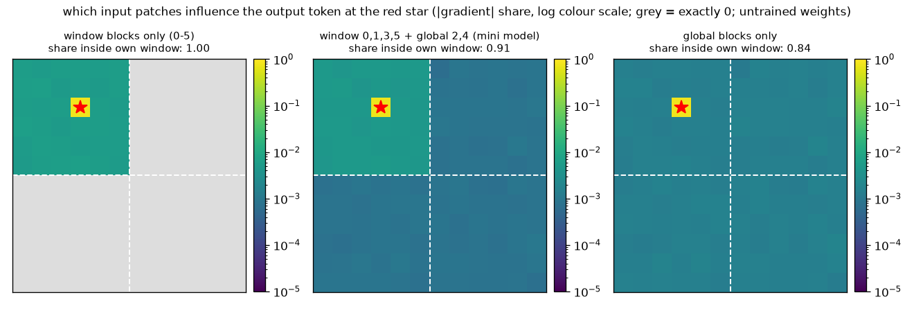
Figure 9-2 looks at the same fact from the other direction. Pick one cell of the output and measure, with gradients, which input patches it depends on.
- Left (window blocks only). Everything outside the top-left window (6×6 cells) containing the star is gray. This cell's output does not change whatever the pixels in other windows are.
- Middle (mini model: window 0, 1, 3, 5 + global 2, 4). There is color outside the window too, but the inside of the window is one shade darker. Patches inside its own window account for 0.91.
- Right (global blocks only). The window boundaries are not visible. The share inside its own window is 0.84.
- Limits in reading this figure
- In all three plots, only the cell with the star stands out in yellow. In an untrained model, because of residual connections, an output cell depends almost entirely on its own patch. That is why even on the right, with only global blocks, its own window accounts for as much as 0.84. This figure does not show where a trained model actually looks; it shows which information flows the structure allows (gray = impossible). Numbers such as 0.91 · 0.84 change after training.
How much accuracy does window attention cost, then? In table 2 of the paper, the row that adds window attention drops mAP by 1.3, from 36.0 to 34.7 (12-epoch training). That is the price of cutting compute to 0.72 times. In this tutorial's shape-world experiment (chapter 11), the AP difference between the 2×2-window model and the all-global model over three seeds was −0.0014, +0.0041, −0.0009 (global − window), small enough that the sign varied. It is a small task with only 1 – 4 shapes per image, so it says nothing about the loss on COCO.
Window-major organization
Window attention reduced the compute. Yet the LW-DETR paper reports that while compute went down, latency actually went up. The cause lay in the order in which the tokens are laid out, and the fix is the implementation technique this paper itself contributed: window-major organization (window-major feature map organization).
The problem with row-major order
When a token grid is flattened into a sequence, it is usually read one row at a time: the first row from left to right, then the next row from left to right. This is row-major order, and the ViT of chapter 6 was flattened this way too. It poses no problem for global attention. But window attention needs the tokens of one window gathered together, and in row-major order the tokens of a window are scattered across the sequence. So a ViTDet-style implementation does the following every time it meets a window block.
- Reorder the tokens to group them by window.
- Compute the window attention block.
- Restore the tokens to their original (row-major) order.
Steps 1 and 3 are not computation but moving values around in memory. In PyTorch terms, it is a reshape after a permute, which copies the whole tensor into the new order. With 6 window blocks, this copy happens 12 times.
Laying out tokens window by window
Window-major organization changes the order only once, at the start. The tokens are laid out by window: all the tokens of the first window, then all the tokens of the next window, and so on. Once this is done, the tokens of a window form a contiguous span of the sequence, so cutting into windows takes only a reshape that moves no values (view).
- Figure: Figure 9-3 The number in each cell is that token's position in the sequence, and the color is its window. Left: row-major order of a 4×4 grid. Middle: window-major order of the same grid. Right: window-major order of the mini model's 12×12 grid divided into 2×2 windows.
- Row-major position numbers of a 4×4 grid, window-major position numbers of the same grid, and window-major position numbers of a 12×12 grid divided into 2×2 windows. Cell color indicates the window.
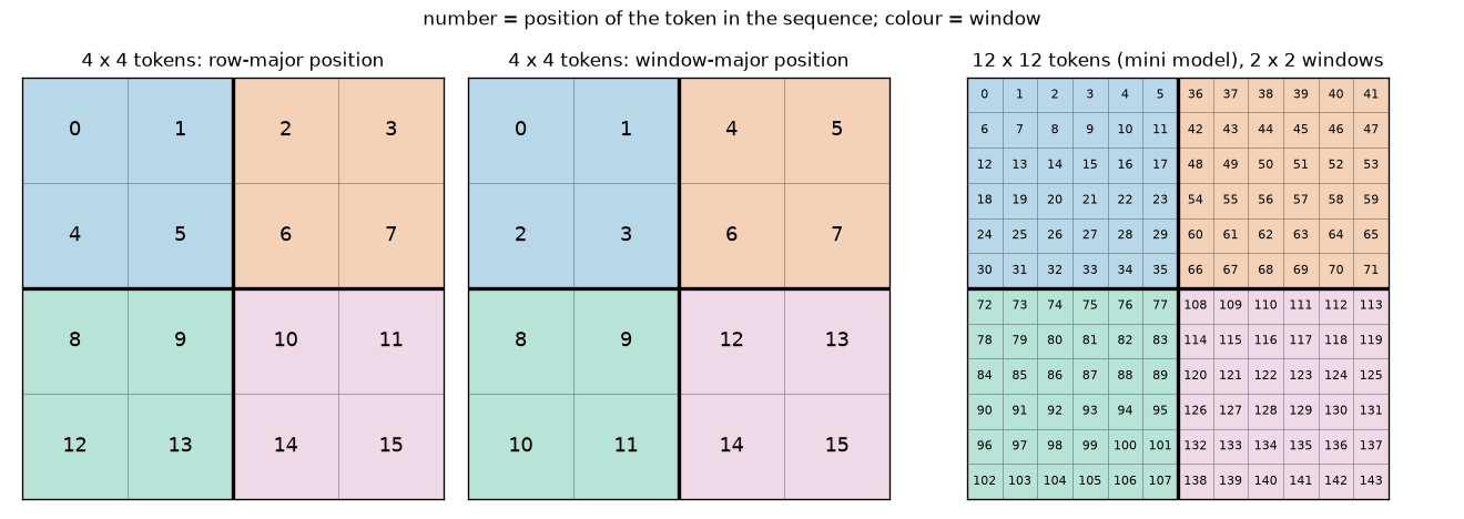
What to read from figure 9-3:
- Left (row-major). The numbers go one row at a time: 0 – 3, 4 – 7, …. The four cells of the blue window are at positions 0, 1, 4, 5, apart from each other in the sequence.
- Middle (window-major). The blue window occupies positions 0 – 3, orange 4 – 7, green 8 – 11, and pink 12 – 15. One window = one contiguous span of the sequence. Simply cutting the sequence into four pieces yields the windows.
- Right. The same holds for the mini model. Each window's 36 cells have consecutive numbers (0 – 35, 36 – 71, 72 – 107, 108 – 143). Both the order of the windows and the order within a window are row-major.
The 4×4 example traced by hand
Section 3.4 of the LW-DETR paper explains this layout with a 4×4 feature map (equations 3 – 5 of the paper). Name the cells \(f_{\text{row}\,\text{col}}\).
\(\begin{bmatrix} f_{11} & f_{12} & f_{13} & f_{14} \\ f_{21} & f_{22} & f_{23} & f_{24} \\ f_{31} & f_{32} & f_{33} & f_{34} \\ f_{41} & f_{42} & f_{43} & f_{44} \end{bmatrix}\)
With 2×2 windows (number of windows per side \(W_n = 2\)), the two layouts are as follows. The semicolons are inserted to split them into groups of four for readability.
\(\begin{aligned} \text{row-major:}\quad & f_{11}, f_{12}, f_{13}, f_{14};\; f_{21}, f_{22}, f_{23}, f_{24};\; f_{31}, f_{32}, f_{33}, f_{34};\; f_{41}, f_{42}, f_{43}, f_{44} \\ \text{window-major:}\quad & f_{11}, f_{12}, f_{21}, f_{22};\; f_{13}, f_{14}, f_{23}, f_{24};\; f_{31}, f_{32}, f_{41}, f_{42};\; f_{33}, f_{34}, f_{43}, f_{44} \end{aligned}\)
The first piece of the window-major order, \(f_{11}, f_{12}, f_{21}, f_{22}\), is the top-left 2×2 window. The function that produces this order is to_window_major.
def to_window_major(tokens: torch.Tensor, grid_h: int, grid_w: int, num_windows: int) -> torch.Tensor:
    """행 우선으로 늘어선 토큰을 윈도 우선으로 다시 늘어놓고, 윈도를 배치 축으로 올린다.

    tokens: (B, H·W, C) — 토큰 격자 H×W 를 한 행씩 읽은 순서 (행 우선, row-major).
    num_windows: 한 변의 윈도 수 W_n. 격자를 W_n × W_n 개 윈도로 나눈다 (H, W 는 W_n 의 배수).
    돌려주는 값: (B·W_n², (H/W_n)·(W/W_n), C) — 윈도 하나가 배치의 한 줄. 윈도 순서도, 윈도 안 순서도 행 우선.
    """
    batch, _, channels = tokens.shape
    win_h, win_w = grid_h // num_windows, grid_w // num_windows  # 윈도 하나의 높이 · 너비 (토큰 수)
    x = tokens.view(batch, num_windows, win_h, num_windows, win_w, channels)  # (B, 윈도 행, 안쪽 행, 윈도 열, 안쪽 열, C)
    x = x.permute(0, 1, 3, 2, 4, 5)  # (B, 윈도 행, 윈도 열, 안쪽 행, 안쪽 열, C) — 여기서 순서가 바뀐다 (복사가 일어난다)
    return x.reshape(batch * num_windows**2, win_h * win_w, channels)

def from_window_major(tokens: torch.Tensor, grid_h: int, grid_w: int, num_windows: int) -> torch.Tensor:
    """to_window_major 의 역연산. (B·W_n², (H/W_n)·(W/W_n), C) → (B, H·W, C) 행 우선."""
    channels = tokens.shape[-1]
    win_h, win_w = grid_h // num_windows, grid_w // num_windows
    x = tokens.view(-1, num_windows, num_windows, win_h, win_w, channels)
    x = x.permute(0, 1, 3, 2, 4, 5)  # (B, 윈도 행, 안쪽 행, 윈도 열, 안쪽 열, C)
    return x.reshape(-1, grid_h * grid_w, channels)

def window_major_order(grid_h: int, grid_w: int, num_windows: int) -> torch.Tensor:
    """윈도 우선 배치에서 k 번째 자리에 오는 토큰의 행 우선 번호. (H·W,) LongTensor."""
    index = torch.arange(grid_h * grid_w, dtype=torch.float32).view(1, -1, 1)
    return to_window_major(index, grid_h, grid_w, num_windows).flatten().long()
The body of the function is three lines: view splits the axes into four, permute swaps the middle two axes, and reshape flattens them again. Let us follow the 4×4 example to see how these three lines produce the window-major order. Counting rows and columns from 0 as \(r, c \in \{0, 1, 2, 3\}\), the row-major index of \(f_{(r+1)(c+1)}\) is \(4r + c\).
- The order produced by view → permute → reshape (4×4 grid, 2×2 windows)
- \(r = 2a + i, \qquad c = 2b + j \qquad (a, b, i, j \in \{0, 1\})\)
- Split the row index \(r\) into "which window row (\(a\))" and "which row within that window (\(i\))". Split the column the same way into window column \(b\) and inner column \(j\). For example, \(r = 3\) is the second row (\(i = 1\)) of the lower window row (\(a = 1\)).
- Substituting the equations above and expanding. This equals the linear index of cell \((a, i, b, j)\) in a 4-dimensional array of size \((2, 2, 2, 2)\). So
view(B, 2, 2, 2, 2, C)moves no values and only names the axes (window row, inner row, window column, inner column).
-
permute(0, 1, 3, 2, 4, 5)swaps the middle two axes (inner row \(i\) and window column \(b\)). Now the first two axes \((a, b)\) say "which window", and the last two \((i, j)\) say "which cell within the window".
- When
reshapeflattens it back into a sequence, cell \((a, b, i, j)\) lands at this index. The four cells sharing window number \(2a + b\) occupy the consecutive positions \(4(2a + b),\ \dots,\ 4(2a + b) + 3\).
- Decomposing the fifth window-major position (\(k = 4\)) gives \(4 = 8 \cdot 0 + 4 \cdot 1 + 2 \cdot 0 + 0\), so it is the first cell of the top-right window (\(b = 1\)). That cell's row-major index is 2, that is, \(f_{13}\) with \(r = 0, c = 2\). This matches the fifth entry being \(f_{13}\) in equation (4) of the paper. In the same way, \(k = 2\) is \((0, 0, 1, 0)\), row-major index 4, that is, \(f_{21}\).
Here is the same example printed by the practice code. Compare it character by character with equations (4) · (5) of the paper.
[윈도 우선 배치] LW-DETR 논문의 4×4 예, 윈도 크기 2×2 (한 변의 윈도 수 2)
  행 우선  : f11, f12, f13, f14; f21, f22, f23, f24; f31, f32, f33, f34; f41, f42, f43, f44
  윈도 우선: f11, f12, f21, f22; f13, f14, f23, f24; f31, f32, f41, f42; f33, f34, f43, f44
  윈도 우선 자리 → 행 우선 번호: [0, 1, 4, 5, 2, 3, 6, 7, 8, 9, 12, 13, 10, 11, 14, 15]
  to_window_major: (1, 16, 1) → (4, 4, 1)  (윈도 4개가 배치 축으로)
  check from_window_major(to_window_major(x)) = x: True
The list on the third line matches the hand calculation: position 4 holds row-major index 2, and position 2 holds row-major index 4. The fourth line shows one 16-token sequence (1, 16, 1) turned into 4 windows × 4 tokens (4, 4, 1). The windows have moved onto the batch axis.
Why global attention still works
Window blocks can now simply be computed as is. The remaining question is the global blocks. Is it all right to run global attention when the tokens are shuffled into window-major order? It is, for two reasons.
- A reshape alone makes it one row. In
(B·W_n², N/W_n², D), the \(W_n^2\) windows of one image are adjacent rows on the batch axis. Since they already sit consecutively in memory,view(B, N, D)turns all the tokens of one image into one row without moving any values. In the mini model, this means viewing(8, 36, 96)as(2, 144, 96). - Self-attention does not care about token order. This is the permutation equivariance of chapter 5. Shuffling the order of the input tokens just shuffles the outputs the same way; each token receives the same value. Position information lives not in the order but in the position embeddings added to the tokens, and the position embeddings are added before the order is changed. So running global attention on tokens in window-major order gives, token by token, the same result as running it on tokens in row-major order.
In short, with window-major organization both window blocks and global blocks run without any reordering. The order is changed only once on entering the encoder and once when taking out the feature map. In the paper's words, this layout "can be used for both window attention and global attention without rearranging features". Here is code implementing the two approaches side by side.
def run_blocks_row_major(blocks, tokens, grid_h, grid_w, num_windows, window_blocks):
    """(a) 행 우선 배치: 토큰은 늘 (B, H·W, C) 로 두고, 윈도 블록을 만날 때마다 순서를 바꿨다가 되돌린다 (ViTDet 방식)."""
    for i, block in enumerate(blocks):
        if i in window_blocks:
            windows = to_window_major(tokens, grid_h, grid_w, num_windows)  # 순서 바꾸기 (복사)
            tokens = from_window_major(block(windows), grid_h, grid_w, num_windows)  # 되돌리기 (복사)
        else:
            tokens = block(tokens)  # 전역 어텐션은 그대로
    return tokens

def run_blocks_window_major(blocks, tokens, grid_h, grid_w, num_windows, window_blocks):
    """(b) 윈도 우선 배치: 들어갈 때 한 번, 나올 때 한 번만 순서를 바꾼다 (LW-DETR · RF-DETR 방식).

    그 사이의 윈도 블록은 그대로, 전역 블록은 view 로 윈도 W_n² 개를 한 줄로 붙여서 계산한다.
    """
    windows = to_window_major(tokens, grid_h, grid_w, num_windows)  # (B·W_n², T_w, C)
    for i, block in enumerate(blocks):
        windows = block(windows, merge=1 if i in window_blocks else num_windows**2)
    return from_window_major(windows, grid_h, grid_w, num_windows)
In (b), global blocks receive merge=num_windows**2. Inside the block, the \(W_n^2\) adjacent rows of the batch are joined into one row with view, attention is run, and afterward view restores them (the block's code is shown in "Reading the implementation"). Let us check that the two approaches give the same values.
[윈도 어텐션] 블록 6개 (윈도 0, 1, 3, 5 / 전역 2, 4), 12×12 토큰, 윈도 2×2
  check (a) 행 우선 + 매번 순서 바꾸기 vs (b) 윈도 우선: 최대 차이 7.15e-07 (출력 평균 절댓값 0.908)
  참고: 모든 블록을 전역으로 돌린 출력과의 차이 5.19e-01 (다른 계산이다)
The difference between (a) and (b) is \(7 \times 10^{-7}\), at the level of 32-bit floating-point rounding. The two approaches compute the same function. What differs is not the values but only the number of memory moves needed to get them. The third line is for comparison: turning all window blocks into global ones changes the output by as much as 0.52. Window attention is not an approximation of global attention but a different computation.
The paper's numbers and this tutorial's measurements
First, what the paper reports. These are the three relevant rows of table 2 of the LW-DETR paper (small model, T4 · TensorRT).
| Setting | Compute | Latency | mAP |
| Global attention only (+ multi-level feature aggregation) | 23.0 GFLOPs | 3.7 ms | 36.0 |
| + interleaved window · global (ViTDet-style implementation, row-major) | 16.6 GFLOPs | 3.9 ms | 34.7 |
| + window-major organization | 16.6 GFLOPs | 2.9 ms | 34.7 |
Compute dropped from 23.0 to 16.6 GFLOPs, yet latency rose by 0.2 ms, from 3.7 to 3.9 ms. The paper attributes this to the cost of the reordering operations needed with row-major order. Switching to window-major organization leaves compute and mAP unchanged and brings latency alone down to 2.9 ms, 0.8 ms less than the original 3.7 ms. The lesson here reaches beyond window attention: less compute (FLOPs) does not mean less time. FLOPs count only multiplications and additions, not the moving of values in memory.
Now for what this tutorial measured. Six blocks (4 window + 2 global, dimension 96) were fed a batch of 8, and three approaches were timed: all blocks global, (a) row-major + reordering, and (b) window-major. To spread fluctuations in GPU state evenly, the three approaches were timed alternately for 40 rounds; the first 8 rounds were discarded and the shortest time was recorded.
  시간 (장치 cuda, 배치 8, 블록 6개, 차원 96, ms) — 세 방식을 번갈아 40바퀴 재고, 앞 8바퀴를 버린 최솟값
  토큰 격자 | 전부 전역 | (a) 행 우선 + 순서 바꾸기 | (b) 윈도 우선 | (a) − (b)
    12×12  |      1.01 |                     0.97 |          0.96 |    +0.01
    24×24  |      5.05 |                     4.10 |          4.06 |    +0.04
    48×48  |     48.88 |                    28.96 |         29.29 |    -0.33
- Figure: Figure 9-4 Left: the number of (query, key) pairs in one attention pass (vertical axis on a log scale). Right: actual time for 6 blocks · batch 8. Blue is all blocks global, orange hatching is (a) row-major + reordering, and green dots are (b) window-major. The numbers above the bars are in ms.
- Left: a log-axis graph of the number of attention pairs versus token grid size, for global and for 2×2, 3×3, 4×4 windows. Right: a bar chart of the actual time of 6 blocks at three grid sizes, measured with the three approaches.
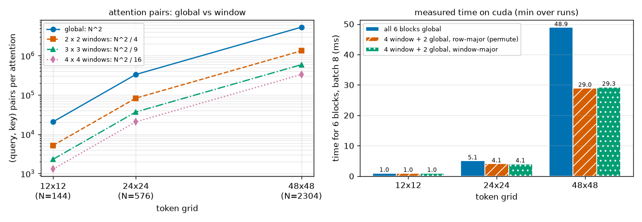
There are two things to read from the table and figure 9-4, and both differ somewhat from what one might expect.
- The speed gain from window attention appeared only for large grids. The pair count on the left of figure 9-4 is 1/4 of global at every grid size, as theory says (orange dashed line). But the time on the right is essentially unchanged at 12×12, 1.01 → 0.97 ms, and is 0.81 times at 24×24 and 0.59 times at 48×48. On the mini model's 12×12 grid, window attention gives no speed gain.
- No time difference between (a) and (b) was measured. The orange and green bars are the same height. (a) − (b) is +0.01, +0.04, −0.33 ms, even mixed in sign, and within the measurement noise. The paper's table 2 result, "3.9 ms because of reordering, 2.9 ms with window-major organization", was not reproduced in this measurement.
Point 1 is explained by "only the quadratic term shrinks" above. Let us estimate by hand.
- Time ratio estimated from multiplication counts (dimension 96, 2×2 windows, 4 window + 2 global)
- \(\text{global block} \;\propto\; 12ND^2 + 2N^2D \;=\; 12ND^2\left(1 + \frac{N}{6D}\right)\)
- Factoring \(12ND^2\) out of chapter 6's estimate. The 1 in the parentheses is the linear layers' share, and \(N/6D\) is the attention pairs' share.
- Only the pairs' share shrinks, to \(1/W_n^2 = 1/4\). The linear layers' share of 1 stays the same.
- The numerator is 2 global + 4 window, the denominator 6 global. The common \(12ND^2\) cancels.
- 12×12 grid. The attention pairs' share is only a quarter of the linear layers', so cutting it to a quarter reduces the total by only 10%.
- 24×24 grid. The size at which the two shares are equal.
- 48×48 grid. Attention pairs take up 80% of a block, so the gain is large. The measured values are, in order, \(0.97/1.01 = 0.96\), \(4.10/5.05 = 0.81\), \(28.96/48.88 = 0.59\). They follow the same trend as the estimates 0.90 · 0.75 · 0.60, and nearly match for the large grid.
That the measured values for the small grids (0.96, 0.81) shrank less than the estimates (0.90, 0.75) appears to be because, for computations this small, time depends more on the number of layers and function calls than on the number of multiplications. Six blocks on a 12×12 grid finish in 1 ms. Real RF-DETR grids start at 24×24 (Nano) and get much larger (the table in chapter 6), so they fall on the side where the gain from window attention shows up.
As for point 2, there are good reasons why no difference between the two layouts was measured.
- What was measured is different. The paper's numbers are the latency of the whole detector converted with TensorRT on a T4 GPU; what was measured here is six blocks run directly in PyTorch.
- Copies are cheap in PyTorch on a GPU. The
permute+reshapecopies (8 round trips for 4 window blocks) are very light compared with the matrix multiplications of attention and the MLP. - The measurement is not that precise. These values were measured on a laptop GPU, so differences on the order of 0.1 ms cannot be read. In a trial run while the GPU was shared with other work, (b) even came out slower. The difference is of a size that flips with load.
- Key points · what was and was not confirmed
-
- Confirmed (code). With window-major organization, the per-block reordering disappears structurally. (a) calls
permutetwice per window block, while (b) calls it only twice in total. The outputs of the two approaches are the same (maximum difference 7.15e-07). - Not confirmed (time). That gain did not show up in measurements on this PC. The paper's reported 3.9 → 2.9 ms is for T4 · TensorRT, and this tutorial did not measure in that environment.
- Seen along the way. Window attention itself gives no speed gain when there are few tokens. "Compute went down" and "it got faster" have to be checked separately.
- Confirmed (code). With window-major organization, the per-block reordering disappears structurally. (a) calls
Projector and C2f
What the projector does
There are three reasons the decoder cannot read the encoder's feature maps directly. The projector solves all three at once.
- The channel counts differ. The encoder dimension (192 for LW-DETR small) differs from the decoder dimension (256), and concatenating several layers multiplies the channels. They must be converted to the channel count the decoder uses.
- Features from several layers must be mixed. Concatenation only places them side by side. A computation is needed that blends the information from shallow and deep layers into one vector per cell.
- Neighboring cells must be looked at together. A ViT token corresponds to a single patch. Gathering information from surrounding cells with 3×3 convolutions yields features better suited to detection. The resolution is also changed here if needed.
LW-DETR uses the C2f block for this. The paper introduces it as "an extension of the CSP (cross-stage partial) structure, implemented in YOLOv8". It takes a convolutional block refined by the YOLO family and places it as is between the DETR encoder and decoder.
Structure of the C2f block
The basic unit of C2f is a "convolution → normalization → activation function" bundle. This is ConvX in the code; the convolution has no bias (the normalization right after it plays the role of the bias), and the activation function is the SiLU of chapter 4. With \(C_{\text{out}}\) output channels, half of that \(c = C_{\text{out}} / 2\), and \(n\) bottlenecks, C2f has four steps.
- A 1×1 convolution (cv1) turns the input into \(2c\) channels. A 1×1 convolution applies the same linear layer to every cell (chapter 4). The resolution stays the same; only the channel count changes.
- The result is split in half along the channel axis. Call the first \(c\) channels \(y_0\) and the last \(c\) channels \(y_1\).
- It passes through \(n\) bottlenecks in sequence: \(y_2 = m_1(y_1)\), \(y_3 = m_2(y_2)\), …, \(y_{n+1} = m_n(y_n)\). One bottleneck (\(m_k\)) is two 3×3
ConvXlayers, and the channel count stays at \(c\). \(y_0\) skips the bottlenecks and passes straight through. - All of \(y_0, y_1, \dots, y_{n+1}\) are concatenated into \((2 + n)c\) channels, and a 1×1 convolution (cv2) reduces them to \(C_{\text{out}}\) channels.
Original figure 9-5 (diagram): The C2f block. The input passes through the 1×1 convolution cv1 and splits into two branches, y0 and y1; y1 goes through three bottlenecks in turn, producing y2, y3, y4. All five branches are concatenated and sent to the 1×1 convolution cv2. The C2f block. The output of cv1 is split in two, only one side (\(y_1\)) goes through the bottlenecks in turn, and the intermediate results \(y_0 \dots y_4\) are all gathered and combined by cv2.
What to look at in figure 9-5 is how the arrows converge.
- Intermediate results are not thrown away. The output of bottleneck 1, \(y_2\), becomes the input of bottleneck 2 and also goes into the final concatenation. Results that passed through 0 bottlenecks (\(y_0\), \(y_1\)), 1 (\(y_2\)), 2 (\(y_3\)), and 3 (\(y_4\)) all reach cv2.
- Shallow and deep paths coexist. Each 3×3 convolution widens the neighborhood a cell sees. \(y_0\) is a feature that has seen only its own cell, while \(y_4\) has passed through six 3×3 convolutions and sees a 13×13 neighborhood. cv2 mixes these five kinds per cell.
- Gradients get a shortcut. There are paths from cv2 to cv1 that pass through no bottleneck at all (\(y_0\), \(y_1\)), so, like the residual connections of chapter 4, gradients also flow along shallow paths.
- There is no residual connection inside the bottleneck
- The
Bottleneckin the code can enable a residual connection that "adds the input", but C2f calls it with this turned off (shortcut=False). That is how RF-DETR's public code does it. So one bottleneck really is just two 3×3 convolutions. The shortcut role is played not by an addition inside the bottleneck but by the concatenation outside it.
Counting channels and parameters
Let us follow the channel counts with this chapter's settings. The input is 288 channels from concatenating three encoder layers, the output is \(C_{\text{out}} = 128\), and there are \(n = 3\) bottlenecks. So \(c = 128 / 2 = 64\).
[프로젝터] 입력: WindowedViT 의 특징 맵 3개, 각각 (2, 96, 12, 12)
  P4 한 단계의 모양 추적 (out_channels = 128, 병목 3개)
    세 층을 채널로 이어 붙임         (2, 288, 12, 12)
    cv1 (1×1) → 2c = 128 채널       (2, 128, 12, 12) → 둘로 나눔: 각각 (2, 64, 12, 12)
    병목 1 (3×3 두 번)              (2, 64, 12, 12)
    병목 2 (3×3 두 번)              (2, 64, 12, 12)
    병목 3 (3×3 두 번)              (2, 64, 12, 12)
    모두 이어 붙임 (2 + 3)·c         (2, 320, 12, 12)
    cv2 (1×1) → 층 정규화            (2, 128, 12, 12)
    check 단계별 계산 = projector(features): 최대 차이 0.00e+00
    매개변수 300,544개
The channels flow \(288 \to 128 \to (64, 64) \to 64 \to 64 \to 64\); gathering the five branches gives \(5 \times 64 = 320\), and at the end it becomes 128. The 12×12 resolution never changes. Let us count the 300,544 parameters on the last line by hand. As seen in chapter 4, a bias-free convolution has (input channels) × (output channels) × (kernel height) × (kernel width) parameters, and layer normalization has one scale and one bias per channel, that is, twice the channel count.
- Parameter count of one projector stage (input 288, output 128, c = 64, 3 bottlenecks)
- \(\text{cv1}:\quad \underbrace{288 \times 128 \times 1 \times 1}_{\text{1×1 conv}} + \underbrace{2 \times 128}_{\text{norm}} = 36{,}864 + 256 = 37{,}120\)
- 288 input channels to \(2c = 128\) channels. With a 1×1 kernel, this equals one \(288 \to 128\) linear layer per cell.
- The convolutions inside a bottleneck go from 64 channels to 64 channels. The 3×3 kernel makes the weights 9 times as many.
- Two 3×3 ConvX per bottleneck, and three bottlenecks.
- The concatenated \((2 + 3) \times 64 = 320\) channels to 128 channels.
- There is one more layer normalization after C2f (the end of the projector stage).
- The same as the count from the code. 74% of the parameters are in the bottlenecks' 3×3 convolutions (\(221{,}952 / 300{,}544 = 0.74\)).
For comparison, this chapter's entire windowed ViT encoder has 705,024. One projector stage is about 43% of the encoder, not a small part.
Single scale and two scales
What we have seen so far is a single-scale projector that outputs the encoder's resolution as is. LW-DETR's tiny · small · medium use this, giving the decoder one feature map at 1/16 of the image resolution. In large and xlarge, the projector outputs feature maps at two resolutions (1/8 and 1/32), and the decoder reads both together with the multi-scale deformable attention of chapter 8. The paper describes it as follows.
- 1/8 map: the input is upsampled 2× with a transposed convolution (deconvolution) and then passes through one C2f block.
- 1/32 map: the input is halved with a strided convolution and then passes through another C2f block.
Since a ViT has only one resolution, other resolutions, when needed, are produced by the projector. Upsampling uses the transposed convolution of chapter 4 (kernel 2, stride 2: each cell unfolds into 2×2 cells), and downsampling uses a 3×3 convolution with stride 2. RF-DETR's public code generalizes this into a list of scale factors, and this chapter's MultiScaleProjector follows that structure: one stage per scale factor, one C2f per stage.
  P3 · P4: 출력 [(2, 128, 24, 24), (2, 128, 12, 12)], 매개변수 638,096개
  P3 · P4 · P5: 출력 [(2, 128, 24, 24), (2, 128, 12, 12), (2, 128, 6, 6)], 매개변수 1,188,048개
The names P3 · P4 · P5 are the detection convention for feature maps at strides 8 · 16 · 32. In the code they mean "the scale factor when the ViT feature map is taken as P4": P3 is 2×, P4 is unchanged, and P5 is half. The mini model's patch size is 8, so the actual strides are half of these (P4 is 12×12), but the scale relationships are the same. From the 12×12 P4, a 24×24 P3 and a 6×6 P5 were produced. Each additional scale adds one more C2f, so the parameters grow by 300K – 550K each time.
We can also count why the P3 stage is a bit larger than the P4 stage (638,096 − 300,544 = 337,552). The transposed convolution upsamples while halving the 96 input channels to 48. There is one for each of the three layers, adding \(3 \times (96 \times 48 \times 2 \times 2 + 48) = 3 \times 18{,}480 = 55{,}440\), and the concatenated channels shrink to \(3 \times 48 = 144\), making cv1 \(144 \times 128 + 256 = 18{,}688\). The rest (bottlenecks, cv2, final normalization) is the same as before, \(221{,}952 + 41{,}216 + 256 = 263{,}424\), so the total is \(55{,}440 + 18{,}688 + 263{,}424 = 337{,}552\).
RF-DETR's default is a single scale with only the P4 stage (projector_scale=["P4"]). For this chapter's multi-scale path, only the shapes of the forward pass were checked; no training was done with it.
From batch normalization to layer normalization
The normalization layer in the middle of ConvX changes between LW-DETR and RF-DETR. LW-DETR's projector uses batch normalization (as section 3 of the RF-DETR paper states). RF-DETR replaced it with layer normalization. As seen by experiment in chapter 4, batch normalization's statistics fluctuate when the batch is small, while layer normalization does not look at other images and so is independent of batch size. The RF-DETR paper gives the reason for this swap as "to enable training on consumer-grade GPUs with gradient accumulation". Gradients from small batches can be accumulated over several steps, but batch normalization statistics cannot (chapter 4).
The code in this chapter follows RF-DETR's public structure (layer normalization). However, nn.LayerNorm normalizes the last axis of a tensor while a feature map has channels on the second axis ((B, C, H, W)), so a small module, ChannelLayerNorm, moves the channel axis to the end and back. In each cell, it normalizes across the \(C\) channels to mean 0 · variance 1.
The values match the built-in function, and after normalization the channel mean per cell is 0 and the standard deviation is 1. ConvX keeps the option of choosing batch normalization (the LW-DETR way) with layer_norm=False, but this tutorial did not experiment with that setting. The normalization layer is named bn in the code because it follows the parameter names of the public implementation; in RF-DETR, what sits in that spot is layer normalization.
IoU-aware BCE loss
From here on, the parts help with training rather than structure. Having cut the decoder to 3 layers, accuracy must be squeezed out of that shallow decoder. The first part is the classification loss. Instead of the focal loss of chapter 8, LW-DETR and RF-DETR use the IoU-aware BCE loss (IA-BCE for short). As the name says, it is a BCE whose classification loss is made "aware" of the IoU. This is the most math-heavy section of the chapter.
Classification and localization go their separate ways
Recall an experiment from chapter 3. Without changing the boxes at all, assigning only the scores differently made AP vary from 0.369 to 0.480. AP75 was 0.153 and 0.393. It was highest when the scores followed the boxes' IoU order and lowest when they were reversed. The conclusion then was this: the more accurate a prediction's box, the higher its score should be.
Yet the losses so far do not teach that. In the set loss of chapters 7 · 8, a prediction matched to a ground truth has a classification target of 1, unconditionally. It makes no difference whether that prediction's box overlaps the ground truth with IoU 0.95 or 0.55. The box losses (L1, GIoU) only correct the box head, and the classification loss does not look at how well the box fits. The two losses are trained separately, unaware of each other. As a result, a prediction that is "confident about the class but sloppy about the box" can get a high score, while the prediction whose box fits best gets pushed back.
This loss comes from reference [3] of the LW-DETR paper, Align-DETR (Cai et al., 2023). That paper calls this phenomenon the "misalignment" between classification score and localization accuracy, and points out that it hurts performance on rank-based metrics such as mAP. The remedy is simple: change the classification target from 1 to a value built from the IoU. The query selection of RT-DETR seen earlier arose from the same concern.
- Origin of the name
- What LW-DETR cites is the first version of Align-DETR (arXiv 2304.07527v1, April 2023), titled "Align-DETR: Improving DETR with Simple IoU-aware BCE loss", which is where the name IA-BCE comes from. Equation (1) of the LW-DETR paper is the same as the equation in this first version. Later revisions of Align-DETR changed the loss's name and form (Align Loss), but LW-DETR and RF-DETR use the form from the first version. As neighboring losses aimed at a similar problem, that paper lists Quality Focal Loss and Varifocal Loss, but this tutorial does not cover their equations.
The paper's equation
Equation (1) of the LW-DETR paper, rewritten in this tutorial's notation, is as follows (the paper's score \(s\) is written as \(p\)).
\(\ell_{\text{cls}} = \sum_{i=1}^{N_{\text{pos}}} \operatorname{BCE}(p_i,\ t_i) \;+\; \sum_{j=1}^{N_{\text{neg}}} p_j^{2}\, \operatorname{BCE}(p_j,\ 0), \qquad t = p^{\alpha}\, u^{1-\alpha}\)
Let us read the symbols one by one.
- Cell. The classification head outputs one logit per class for each query (the sigmoid classification without ∅ from chapter 8). One (query, class) pair will be called a cell. With 300 queries and 80 classes there are 24,000 cells, and each cell has one probability \(p\) for "is this query an object of this class".
- Positive cells (\(N_{\text{pos}}\) of them): the cell for that ground truth's class in a query matched to a ground truth by Hungarian matching. There is one positive cell per ground truth.
- Negative cells (\(N_{\text{neg}}\) of them): all the rest. Not only all cells of unmatched queries but also the other-class cells of matched queries are negative.
- \(\operatorname{BCE}(p, t) = -t \log p - (1 - t) \log(1 - p)\): the soft-target BCE of chapter 4. When the target is 0, only \(\operatorname{BCE}(p, 0) = -\log(1 - p)\) remains.
- \(u\): the IoU between the predicted box output by that positive cell's query and its matched ground-truth box (the pairwise IoU of chapter 2). A number between 0 and 1.
- \(t\): the target of a positive cell, built from the current score \(p\) and the IoU \(u\). \(\alpha\) is the exponent that sets the mixing ratio of the two, and the paper uses 0.25. Then \(t = p^{0.25}\, u^{0.75}\).
Two things differ from the loss of chapter 8. The target of positive cells changed from 1 to \(t\), and negative cells are multiplied by \(p^2\). Let us look at each in turn.
Reading the target t
\(t = p^{\alpha} u^{1-\alpha}\) is a weighted geometric mean of \(p\) and \(u\). Where the arithmetic mean \(\alpha p + (1 - \alpha) u\) mixes by adding, the geometric mean mixes by multiplying. First, let us check where \(t\) falls.
- The target \(t\) always lies between \(p\) and \(u\) (\(0 \lt \alpha \lt 1\))
- \(p = p^{\alpha} \cdot p^{1-\alpha}\)
- The exponents add up to \(\alpha + (1 - \alpha) = 1\), so \(p\) itself can be split this way. The same goes for \(u = u^{\alpha} \cdot u^{1-\alpha}\).
- Powers of positive numbers preserve order (\(1 - \alpha \gt 0\)). Both sides were multiplied by the same positive number \(p^{\alpha}\). So \(p \lt t\).
- In the same way, this time multiplying by \(u^{1-\alpha}\). So \(t \lt u\).
- When \(p \gt u\), all the inequalities flip. If \(p = u\), then \(t = p^{\alpha} p^{1-\alpha} = p\). The target is always a point between the current score and the IoU, and coincides with them only when the two are equal.
Let us plug in a few numbers (\(\alpha = 0.25\)).
| Score \(p\) | IoU \(u\) | \(p^{0.25}\) | \(u^{0.75}\) | Target \(t\) | Reading |
| 0.60 | 0.80 | 0.8801 | 0.8459 | 0.7445 | Score below IoU → target above score (raise it) |
| 0.90 | 0.50 | 0.9740 | 0.5946 | 0.5791 | Score above IoU → target below score (lower it) |
| 0.20 | 0.90 | 0.6687 | 0.9240 | 0.6179 | Very good box but low score → raise it a lot |
| 0.50 | 0.50 | 0.8409 | 0.5946 | 0.5000 | Score = IoU → target = score (unchanged) |
The exponent is 0.75 on the \(u\) side and 0.25 on the \(p\) side, so \(t\) is pulled closer to \(u\). Still, since \(p\) is mixed in, when the score is very low the target does not jump all the way to the IoU at once (third row: IoU 0.90 but target 0.62). Looking at the two extremes of \(\alpha\) makes the meaning clear. This is Align-DETR's explanation.
- If \(\alpha = 0\), \(t = u\). The target is entirely the IoU.
- If \(\alpha = 1\), \(t = p\). The target is the current score itself, so there is no learning signal.
- Values in between are a trade-off between "how much the IoU leads" and "training stability", and that paper reports that 0.25 worked well. Its conclusion is that \(\alpha\) should be kept small.
There is one more convention. \(t\) is built from \(p\), but when differentiating the loss, \(t\) is treated as a constant (the stop-gradient of chapter 8). No gradient flows through the \(p\) inside \(t\). A "target" is something to hit, not a variable that moves on its own to reduce the loss. The paper's equation does not mark this, but the implementation does it this way.
The fixed point: the score is pulled toward the IoU
Now let us derive where this loss takes the score. Chapter 4 showed two things: a BCE with a fixed target \(t\) is smallest at \(p = t\), and its gradient with respect to the logit \(z\) is \(p - t\). In IA-BCE, that \(t\) moves with \(p\).
- The gradient of a positive cell is zero at \(p = u\)
- \(\frac{\partial\, \operatorname{BCE}(p, t)}{\partial z} = p - t\)
- The result from chapter 4 (\(p = \sigma(z)\)), differentiating with \(t\) treated as a constant. If \(p \lt t\) the gradient is negative, so gradient descent increases \(z\) and raises \(p\); if \(p \gt t\) it lowers it.
- After differentiating, the value of \(t\), \(p^{\alpha} u^{1-\alpha}\), is substituted. The order matters: substituting first and then differentiating would also differentiate the \(p\) inside \(t\) and give a different expression.
- Find where the gradient is 0 and the score stops moving: where "score = target".
- Both sides divided by \(p^{\alpha}\) (allowed since \(p \gt 0\)). The left side is \(p / p^{\alpha} = p^{1-\alpha}\).
- Both sides raised to the power \(1/(1 - \alpha)\) (\(\alpha \lt 1\)). The gradient is 0 at only one place, where the score equals the IoU.
- The previous section showed that \(p \lt u\) implies \(p \lt t\). So a score below the IoU goes up and one above it goes down. Whichever side it starts from, it heads toward \(p = u\).
Such a point is called a fixed point: once there, it no longer moves. Here it is a fixed point that pulls in from both sides. Compare it with chapter 4's "the minimum is at \(p = t\)" and the difference shows. There the target \(t\) was fixed; now the target moves with the score. When the score goes up, the target goes up a little, and the score follows again. This chase stops at \(p = t\), that is, \(p = u\).
Let us watch the target move with numbers. Suppose the IoU is \(u = 0.8\) and the score starts at \(p = 0.2\). If each update raised the score all the way to the current target (actual training moves in smaller steps), the score would go \(0.2 \to 0.566 \to 0.734 \to 0.783 \to 0.796 \to 0.799 \to 0.800\). The first target is \(0.2^{0.25} \times 0.8^{0.75} = 0.6687 \times 0.8459 = 0.566\), and the next is \(0.566^{0.25} \times 0.8459 = 0.734\). The target approaches 0.8 without ever overshooting the IoU.
Here are the gradients computed by the practice code with autograd. A single positive cell was fed into the loss function and differentiated with respect to the logit.
  IoU = 0.5: p = 0.20: t = 0.3976, ∂손실/∂로짓 = -0.1976 | p = 0.50: t = 0.5000, ∂손실/∂로짓 = +0.0000 | p = 0.95: t = 0.5870, ∂손실/∂로짓 = +0.3630
  IoU = 0.9: p = 0.20: t = 0.6179, ∂손실/∂로짓 = -0.4179 | p = 0.90: t = 0.9000, ∂손실/∂로짓 = +0.0000 | p = 0.95: t = 0.9122, ∂손실/∂로짓 = +0.0378
  → 로짓에 대한 기울기는 p − t. p < IoU 면 음수(점수를 올린다), p > IoU 면 양수(내린다), p = IoU 에서 0.
Check the first entry of the first line by hand: \(t = 0.2^{0.25} \times 0.5^{0.75} = 0.6687 \times 0.5946 = 0.3976\), and the gradient is \(p - t = 0.2 - 0.3976 = -0.1976\). Same as the output. Comparing the two lines, for the same score of 0.95, a box with IoU 0.5 gets a strong "lower it" of \(+0.3630\), while a box with IoU 0.9 gets hardly anything, \(+0.0378\). With ordinary BCE (target 1), both cases would have had a gradient of \(0.95 - 1 = -0.05\), meaning "raise it further".
- Key point · what IA-BCE teaches
- An ordinary classification loss pushes the score of a matched prediction toward 1. IA-BCE pulls that score toward that prediction's IoU. Predictions with well-fitting boxes stop at high scores, sloppy ones at low scores. So the order of the scores comes to resemble the order of box quality, which, as seen in chapter 3, favors AP. In effect, the classification head learns to answer not only "is this the right class" but also "how well does my box fit".
- What this derivation does not say
-
- The IoU moves too. The derivation held \(u\) fixed, but during training the box loss corrects the boxes, so \(u\) rises as well. The score follows the rising IoU.
- The loss does not go to 0. At the fixed point \(p = u\), the loss is \(-u \log u - (1 - u) \log(1 - u)\). For \(u = 0.9\) that is \(0.0948 + 0.2303 = 0.3251\). As seen in chapter 4, a soft-target BCE does not have a minimum of 0. A classification loss that stops falling does not mean training has stalled (this is visible in the training logs of chapter 14).
- A network cannot fit one cell in isolation. The derivation assumed one logit could move freely. In reality, the same weights must fit every cell of every image together, so the score does not become exactly equal to the IoU. How close it gets is measured in chapter 11.
Negative cells take the same form as the focal loss
The second term of the equation, \(p^2\, \operatorname{BCE}(p, 0) = -p^2 \log(1 - p)\), looks familiar. In the focal loss of chapter 4, a negative cell (\(y = 0\)) has \(p_t = 1 - p\) and \(\alpha_t = 1 - \alpha\), so
\(\mathrm{FL}_{\text{neg}} = -(1 - \alpha)\,\big(1 - (1 - p)\big)^{\gamma} \log(1 - p) = -(1 - \alpha)\, p^{\gamma} \log(1 - p)\)
(with \(\gamma = 2\) and the focal loss \(\alpha = 0.25\), this is \(-0.75\, p^2 \log(1 - p)\)). The negative term of IA-BCE is this with only the balancing weight \(0.75\) removed. The modulating factor \(p^2\) plays the same role as in chapter 4. Negative cells are overwhelmingly numerous and mostly easy (\(p\) near 0). \(p^2\) erases the loss from such cells so that the rare positive cells are not buried under the sum of negatives.
Why is no modulating factor used for positive cells? Align-DETR's explanation is this: in DETR, positives are so rare that they should not be discounted as "easy positives" but have their influence preserved, while only the negatives keep the focal-loss weight \(p^2\) so as to focus on hard negatives. So the loss is asymmetric: BCE without a modulating factor for positives, and the focal form for negatives.
- Logit gradient of a negative cell
- \(L = -p^{2} \log(1 - p), \qquad \frac{\partial L}{\partial p} = -2p \log(1 - p) + \frac{p^{2}}{1 - p}\)
- The product rule. Differentiating \(p^2\) gives \(2p\), and differentiating \(-\log(1 - p)\) gives \(1/(1 - p)\). Here \(p^2\) is differentiated too. Unlike the target \(t\), the modulating factor has no stop-gradient (that is how the public implementation does it, as did the focal loss of chapter 4).
- The chain rule. The derivative of the sigmoid is \(\partial p / \partial z = p(1 - p)\) (chapter 4).
- Multiplying out and simplifying. The second term is \(\frac{p^2}{1-p} \cdot p(1-p) = p^3\). Both terms are non-negative, so the gradient is always positive, that is, always "lower the score". The gradient of ordinary BCE is \(p\).
Plug in numbers and compare with ordinary BCE.
| \(p\) | BCE loss \(-\log(1-p)\) | IA-BCE negative loss | BCE gradient \(p\) | IA-BCE negative gradient |
| 0.01 | 0.0101 | 0.000001 | 0.01 | 0.000003 |
| 0.10 | 0.1054 | 0.0011 | 0.10 | 0.0029 |
| 0.40 | 0.5108 | 0.0817 | 0.40 | 0.1621 |
| 0.90 | 2.3026 | 1.8651 | 0.90 | 1.1020 |
Checking the \(p = 0.4\) row by hand, the loss is \(0.16 \times 0.5108 = 0.0817\) and the gradient is \(2 \times 0.16 \times 0.6 \times 0.5108 + 0.064 = 0.0981 + 0.064 = 0.1621\). For a negative that is already well predicted (\(p = 0.01\)), the loss shrinks to about 1/10,000 of ordinary BCE and the gradient to about 1/3,000. Conversely, for a badly wrong negative (\(p = 0.9\)), the gradient is \(1.10\), actually larger than ordinary BCE's \(0.90\). This is exactly the observation of chapter 4: erase the easy cells and put the effort on the hard ones.
Matching the official implementation line by line
RF-DETR's public code writes this loss in terms of two "weights". For each cell, it sets a positive weight \(w_{\text{pos}}\) multiplying \(\log p\) and a negative weight \(w_{\text{neg}}\) multiplying \(\log(1 - p)\), and uses the same expression for every cell.
\(\text{cell loss} = -\,w_{\text{pos}} \log p \;-\; w_{\text{neg}} \log(1 - p)\)
| Cell | \(w_{\text{pos}}\) | \(w_{\text{neg}}\) | Cell loss | Term in the paper's equation (1) |
| Positive cell (matched query · ground-truth class) | \(t\) | \(1 - t\) | \(-t \log p - (1 - t)\log(1 - p)\) | \(\operatorname{BCE}(p, t)\) |
| All other cells | \(0\) | \(p^{\gamma}\) (\(\gamma = 2\)) | \(-p^{2} \log(1 - p)\) | \(p^{2}\, \operatorname{BCE}(p, 0)\) |
The fourth and fifth columns of the table are the same, so the implementation computes the paper's equation as written. There are four implementation details not stated in the paper.
- Stop-gradient. \(t\) becomes a constant via
detach(). The negative weight \(p^{\gamma}\) is not detached. - A floor on the target. If \(t\) is below 0.01 it is raised to 0.01 (
clamp(min=0.01)). If a box does not overlap its ground truth at all, \(u = 0\) and so \(t = 0\), which would make the positive cell indistinguishable from a negative one. The floor leaves a minimal "raise it" signal on matched cells. - The divisor. The paper's equation shows only the sum, but the implementation sums the loss over all cells and divides by the number of ground truths (
num_boxes). When query groups are used, it is the number of ground truths × the number of groups (next section). - Gradient of the IoU. \(u\) is computed from the predicted box but passes no gradient. The classification loss does not correct the box head; boxes are learned only through the box loss.
def ia_bce_loss(logits: torch.Tensor, matched, tgt_classes: torch.Tensor, ious: torch.Tensor, num_boxes: float,
                alpha: float = 0.25, gamma: float = 2.0) -> torch.Tensor:
    """IoU 인지 BCE 손실 (IA-BCE). RF-DETR 공식 구현 criterion.py 의 loss_labels (ia_bce_loss=True) 와 같은 계산.

    logits       (B, N, K)  클래스별 로짓 (시그모이드 방식, ∅ 칸 없음)
    matched      (batch_idx, query_idx) — 각각 (M,). 매칭된 예측은 logits[batch_idx[k], query_idx[k]]
    tgt_classes  (M,)  그 예측의 짝인 정답의 클래스
    ious         (M,)  그 예측 박스와 짝 정답 박스의 IoU (기울기 없음)
    num_boxes    손실을 나눌 수 (배치의 정답 수 × 질의 묶음 수)

    p = σ(로짓). 칸 (b, n, c) 마다
      매칭된 칸 (짝 정답의 클래스 칸):  목표 t = p^α · IoU^(1−α)  (최소 0.01, 기울기 차단)
                                        손실 = −t·log p − (1 − t)·log(1 − p)          ← 목표가 t 인 BCE
      그 밖의 모든 칸:                  손실 = −p^γ · log(1 − p)                        ← p^γ 로 가중한 "목표 0" BCE
    전부 더해 num_boxes 로 나눈다.
    """
    prob = logits.sigmoid()
    batch_idx, query_idx = matched
    pos_weights = torch.zeros_like(logits)  # log p 에 곱할 가중치: 매칭된 칸만 t, 나머지 0
    neg_weights = prob**gamma  # log(1 − p) 에 곱할 가중치: 기본 p^γ (기울기가 흐른다)
    target = prob[batch_idx, query_idx, tgt_classes].pow(alpha) * ious.pow(1 - alpha)
    target = target.clamp(min=0.01).detach()  # 목표는 상수로 본다 (기울기 차단)
    pos_weights[batch_idx, query_idx, tgt_classes] = target
    neg_weights[batch_idx, query_idx, tgt_classes] = 1 - target
    # −pos·log p − neg·log(1 − p) 를 수치적으로 안정되게: log(1 − p) = log σ(−x) = log σ(x) − x
    loss = neg_weights * logits - F.logsigmoid(logits) * (pos_weights + neg_weights)
    return loss.sum() / num_boxes
The final computation in the code, neg_weights * logits - F.logsigmoid(logits) * (pos_weights + neg_weights), is the expression above rewritten in the numerically stable form of chapter 4. When \(p\) is very close to 0 or 1, computing \(\log p\) or \(\log(1 - p)\) directly gives large errors.
- The form computed directly from the logit
- \(1 - p = 1 - \frac{1}{1 + e^{-z}} = \frac{e^{-z}}{1 + e^{-z}} = e^{-z}\, p\)
- Substituting \(p = \sigma(z) = 1/(1 + e^{-z})\) and combining over a common denominator. The last equality regroups \(\frac{1}{1 + e^{-z}} = p\).
- Taking the log of both sides: \(\log(e^{-z} p) = -z + \log p\).
- Substituted into the cell loss.
- Grouping the \(\log p\) terms. This is the same as the line of code.
F.logsigmoidcomputes \(\log \sigma(z)\) stably even for large \(|z|\).
Computing the loss by hand
Let us compute a small example all the way through: one image with 3 queries and 3 classes, and 2 ground truths. Hungarian matching paired query 0 with ground truth A (class 1) and query 1 with ground truth B (class 0); query 2 is unmatched. The IoUs of the two matched boxes are 0.80 and 0.50. The probabilities \(p\) for each cell are as follows (bold cells are positive).
| Class 0 | Class 1 | Class 2 | Match | |
| Query 0 | 0.10 | 0.60 | 0.05 | Ground truth A (class 1), IoU 0.80 |
| Query 1 | 0.90 | 0.20 | 0.02 | Ground truth B (class 0), IoU 0.50 |
| Query 2 | 0.03 | 0.40 | 0.01 | None |
- IA-BCE by hand: 9 cells, 2 positive
- \(t_{A} = 0.60^{0.25} \times 0.80^{0.75} = 0.8801 \times 0.8459 = 0.7445\)
- Target of the positive cell (query 0, class 1). \(0.60^{0.25} = e^{0.25 \ln 0.6} = e^{-0.1277} = 0.8801\), \(0.80^{0.75} = e^{0.75 \ln 0.8} = e^{-0.1674} = 0.8459\).
- BCE with target \(t_A\). The score 0.60 is below the target 0.74, so this loss says "raise it".
- Target of the positive cell (query 1, class 0). The score is high at 0.90, but the IoU is 0.50, so the target is 0.58.
- The second term is large. The \(1 - t_B = 0.42\) portion of the target is "negative", but the score is 0.90, so it incurs a penalty of \(-\log(1 - p) = 2.30\). This loss says lower the score.
- The remaining seven cells. The cell with \(p = 0.40\) accounts for almost all of it at \(0.16 \times 0.5108 = 0.0817\); \(p = 0.20\) gives \(0.04 \times 0.2231 = 0.0089\); and the other five cells (\(p \le 0.10\)) total 0.0012. The dots stand for the three cells with \(p = 0.03, 0.02, 0.01\), which sum to 0.00004.
- Add everything up and divide by the number of ground truths, 2.
[IA-BCE] 손계산 예: 질의 3개 × 클래스 3개. 질의 0 ↔ 정답(클래스 1, IoU 0.80), 질의 1 ↔ 정답(클래스 0, IoU 0.50)
  질의 0 의 p = 0.10, 0.60, 0.05
  질의 1 의 p = 0.90, 0.20, 0.02
  질의 2 의 p = 0.03, 0.40, 0.01
  매칭된 칸 (질의 0, 클래스 1): p = 0.60, IoU = 0.80 → t = 0.60^0.25 · 0.80^0.75 = 0.8801 · 0.8459 = 0.7445
      손실 = −t·log p − (1 − t)·log(1 − p) = 0.3803 + 0.2341 = 0.6144
  매칭된 칸 (질의 1, 클래스 0): p = 0.90, IoU = 0.50 → t = 0.90^0.25 · 0.50^0.75 = 0.9740 · 0.5946 = 0.5791
      손실 = −t·log p − (1 − t)·log(1 − p) = 0.0610 + 0.9691 = 1.0301
  그 밖의 칸 (질의 1, 클래스 1): p = 0.20 → −p²·log(1 − p) = 0.0400 · 0.2231 = 0.0089
  그 밖의 칸 (질의 2, 클래스 1): p = 0.40 → −p²·log(1 − p) = 0.1600 · 0.5108 = 0.0817
  그 밖의 칸 7개의 합 = 0.0919 (p 가 작은 칸은 거의 0)
  전체 = (1.6445 + 0.0919) / 정답 2개 = 0.8682
  check 손계산 0.868188 vs ia_bce_loss 0.868188
  check 무작위 (4, 12, 3) 로짓: ia_bce_loss 15.278476 vs F.binary_cross_entropy 로 다시 계산 15.278473 (차이 2.86e-06)
The hand calculation and the function agree at 0.868188, and on random inputs the value also matches a recomputation with PyTorch's built-in BCE. There are three things to read from this example.
- The higher-scoring side got the larger loss. Query 1 is confident with a score of 0.90, but its box has IoU 0.50, so its loss is 1.03. With ordinary BCE (target 1), it would have been \(-\log 0.9 = 0.105\), almost no penalty. Query 0 has a low score of 0.60 but a good box (IoU 0.80), and its loss is 0.61. With ordinary BCE it would be \(-\log 0.6 = 0.511\).
- The seven negative cells account for 5% of the total (\(0.0919 / 1.7364\)), and nearly all of that comes from the single cell with \(p = 0.40\). \(p^2\) has erased the easy negatives.
- The 0.40 of query 2 is a cell that "nearly became a false prediction". An unmatched query is giving 0.40 to class 1. The negative term pushes this cell down, reducing duplicate and false predictions. This is the classification half of the principle, seen in chapter 7, by which duplicates disappear without NMS.
Seeing it as curves
- Figure: Figure 9-6 Left: the target \(t = p^{0.25} u^{0.75}\) plotted as a function of the score \(p\) (IoU 0.3 · 0.5 · 0.7 · 0.9). Middle: the logit gradient of a positive cell, \(p - t\). Right: the loss of a negative cell (vertical axis on a log scale).
- Left: curves of the target t as a function of the score p for four IoU values, with the line t = p. Middle: curves of the positive-cell logit gradient p − t, with the gradient line of ordinary BCE. Right: a log-axis graph of the negative-cell loss for ordinary BCE, IA-BCE, and the focal loss.
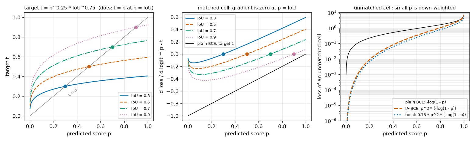
- Left. The four curves are the targets for four boxes with different IoUs. The gray line is \(t = p\). Where a curve is above the line, the target is above the score, so the score rises; where it is below, the score falls. The points where the curves meet the line (circles) are the fixed points, and their horizontal coordinates are exactly the IoUs (0.3, 0.5, 0.7, 0.9). The derived \(p = u\) is visible in the figure. The curves shoot up steeply near \(p = 0\) because of \(p^{0.25}\). Even when the score is very low, like 0.01, the target is set much higher (for IoU 0.9, \(0.01^{0.25} \times 0.9^{0.75} = 0.3162 \times 0.9240 = 0.292\)). Recalling that scores at the start of training are around 0.01 because of the prior-probability bias initialization of chapter 4, this means a generous "raise it" signal applies from the very beginning.
- Middle. The same content drawn as gradients. Each curve crosses 0 at \(p = \text{IoU}\), negative to the left (raise it) and positive to the right (lower it). The black line is the gradient of ordinary BCE (target 1), \(p - 1\). It is always negative and only pushes the score toward 1. The lower a box's IoU (solid blue line), the larger the positive gradient applied to high scores.
- Right. The loss of negative cells. Compared with the black line (ordinary BCE), the orange dashed line (IA-BCE) is cut more the smaller \(p\) is. At \(p = 0.1\), ordinary BCE gives 0.105 and IA-BCE 0.0011, 1/100 as much. The blue dotted line (the negative side of the focal loss) is the orange dashed line times 0.75, so on the log scale it runs parallel, slightly below. The negative sides of the two losses have the same shape.
A preview of the ablation results in chapter 11
Whether "the score follows the IoU" actually happens in training is checked in chapter 11. Here are just the results first. In the shape world, the mini RF-DETR was trained with the same structure and the same settings, changing only the classification loss between IA-BCE and the focal loss (4,000 training images, 15 epochs, three seeds; focal loss coefficient 1).
| Measured (seeds 0 / 1 / 2) | IA-BCE | Focal loss |
| Validation AP | 0.9180 / 0.9210 / 0.9163 | 0.9144 / 0.9103 / 0.9136 |
| Rank correlation between score and IoU (Spearman) | +0.659 / +0.631 / +0.667 | +0.215 / +0.318 / +0.240 |
| Mean |score − IoU| | 0.035 / 0.040 / 0.036 | 0.140 / 0.165 / 0.159 |
| Mean score (mean IoU is about 0.945 for both) | 0.935 / 0.926 / 0.930 | 0.808 / 0.783 / 0.788 |
- The meaning of the score changes. In the model trained with IA-BCE, the mean score (0.93) is nearly equal to the mean IoU (0.945), and the rank correlation between score and IoU is +0.63 – +0.67. The fixed point \(p = u\) actually shows up. Switching to the focal loss collapses the correlation to +0.22 – +0.32, and the scores stay at 0.78 – 0.81 regardless of IoU.
- Yet the AP difference is small. Over the three seeds, focal − IA-BCE is −0.0036, −0.0107, −0.0028. The direction always favors IA-BCE, but the size is similar to how much AP varies across seeds (0.9163 – 0.9210). This appears to be because the shape world has only 1 – 4 shapes per image and most boxes have IoU above 0.9, so there is little to gain from fixing the ranking.
The values the papers report on COCO are larger. In LW-DETR's table 2, the row that adds the IoU-aware classification loss raises mAP by 0.7, from 34.7 to 35.4. The first version of Align-DETR reports that the Pearson correlation between score and IoU rose from 0.483 with the focal loss to 0.597 with IA-BCE. This tutorial's experiment and the papers' experiments differ in both data and model, so the numbers cannot be compared directly; all that can be said is that the direction is the same.
Group DETR
The second training technique increases the amount of supervision signal. The LW-DETR paper describes it in one paragraph under the heading "more supervision": it uses Group DETR (Chen et al., 2022; ICCV 2023), with 13 parallel weight-sharing decoders during training, and only the first one used at inference.
Positives are too rare
The one-to-one matching of chapter 7 pairs only one prediction with each ground truth. That is what made duplicate predictions disappear and NMS unnecessary. The price is sparse supervision. With 300 queries and 5 ground truths in an image, only 5 queries receive the "hit this ground truth" signal (the positive classification target and the box loss). The other 295 learn only "not you". The box head receives gradients for only 5 boxes per image.
Detectors like YOLO are different. They use one-to-many assignment, labeling several nearby locations as positive for each ground truth, and erase the resulting duplicates with NMS. The supervision is plentiful, but NMS is required. The question the Group DETR paper asks is this: can we get the plentiful supervision of one-to-many assignment while keeping NMS-free inference?
Why not just pair several queries with each ground truth? That paper actually tried this "naive one-to-many assignment" and reports that it does not work (table 7 of the paper: a baseline of 32.6 mAP drops to 8.4). The model is trained to output several predictions per ground truth, but there is no mechanism to keep one and lower the scores of the rest, so the duplicate predictions remain.
Separate one-to-one matching per group
Group DETR's answer is to keep several complete sets of queries.
- Keep \(G\) groups of \(N_q\) queries each, \(G \cdot N_q\) queries in total. Each group has its own learned query embeddings.
- All queries pass through the same decoder (the same weights) and produce predictions.
- Hungarian matching is solved separately for each group. Within one group, it is exactly the one-to-one matching of chapter 7.
- The losses of all groups are added up for training.
- At inference, only the first group is used.
From the ground truth's side, each group provides one match, so each ground truth is paired with \(G\) predictions. The positives per image grow from \(T\) to \(G \cdot T\). With 13 groups and 5 ground truths, positives go from 5 to 65. Overall it is one-to-many assignment, but within each group it is still one-to-one. That paper calls it "group-wise one-to-many assignment".
Original figure 9-7 (diagram): Group DETR. Three query groups pass through the same decoder to produce predictions, and each group is separately matched one-to-one with two ground truths. Self-attention happens only within a group, and only the first group is used at inference. Group DETR (example with 3 groups, 4 queries per group, and 2 ground truths). Because each group is matched one-to-one separately, ground truths A and B each get three matches.
Count the lines in figure 9-7. Three lines reach ground truth A and three reach B. Within one group (same color), only one line goes to A and one to B. The Group DETR paper interprets this structure in two ways. One is that it is equivalent to training \(G\) weight-sharing decoders in parallel (the "13 parallel decoders" in the LW-DETR paper refers to this); the other is that it acts like data augmentation for the queries, having different query groups solve the same image with the same ground truths several times.
Here is the per-group matching from the practice code: 4 groups of 12 queries, and two images with 2 and 3 ground truths (long lines are wrapped).
  묶음별 매칭 (질의 12 × 묶음 4, 그림 2장 · 정답 2개 / 3개)
    그림 0: 짝 8개 = 정답 2개 × 묶음 4개: 1(묶음 0)→정답 1, 8(묶음 0)→정답 0, 14(묶음 1)→정답 1, 20(묶음 1)→정답 0,
            29(묶음 2)→정답 0, 34(묶음 2)→정답 1, 40(묶음 3)→정답 0, 46(묶음 3)→정답 1
    그림 1: 짝 12개 = 정답 3개 × 묶음 4개: 4(묶음 0)→정답 1, 5(묶음 0)→정답 2, 8(묶음 0)→정답 0, 13(묶음 1)→정답 1,
            15(묶음 1)→정답 2, 23(묶음 1)→정답 0, 26(묶음 2)→정답 2, 28(묶음 2)→정답 1, 32(묶음 2)→정답 0,
            38(묶음 3)→정답 1, 39(묶음 3)→정답 2, 45(묶음 3)→정답 0
  check 묶음을 하나씩 떼어 7장 HungarianMatcher 로 매칭한 결과와 같은가: True
Query indices run 0 – 47, and the queries of group \(g\) are \(12g\) through \(12g + 11\). In image 0, ground truth 0 was paired with queries 8 (group 0), 20 (group 1), 29 (group 2), and 40 (group 3), and ground truth 1 with 1, 14, 34, 46: exactly once per group. The last line confirms that this matching is the same as "taking the groups one at a time and running chapter 7's matching four times". There is no new algorithm; the cost matrix is simply cut by group and the Hungarian problem solved several times.
The divisor of the loss changes too. The previous section said the classification loss is divided by the number of ground truths; with groups, it is divided by the number of ground truths × the number of groups. The positives became \(G\) times as many, so the divisor is \(G\) times as large too. The loss magnitude thus becomes "the average loss per group", independent of the number of groups.
Groups do not see each other
One more thing is needed. In the decoder layers' self-attention, queries from different groups must be kept from seeing each other. Cross-attention and the FFN are computed per query, so nothing needs to change there; self-attention is the only place where queries mix.
Why block it? As seen in chapter 7, DETR removes duplicate predictions through "one-to-one matching + self-attention among queries". Through self-attention, a query finds out what other queries have taken on, and learns to lower its own score if another query has already taken an object. Now suppose the queries of group 0 could also see the queries of group 1. The query that took ground truth A in group 0 and the one that took it in group 1 are both positive; both must output high scores. The rule "back off if someone else has it" clashes with the demand "output a high score even if someone else has it". Duplicate suppression must not happen between groups, but if they can see each other, it does.
Consistency with inference is also at stake. At inference there is only the first group. If the first group's queries were computed while looking at other groups during training, at inference they would perform a computation never done in training. If groups do not see each other, the first group's computation is the same whether or not other groups exist, and training really becomes "running several independent decoders side by side that share only their weights".
The Group DETR paper's explanation runs along the same lines: since one-to-one matching happens within a group, information among predictions only needs to be gathered within the same group, and self-attention split that way removes the influence of other groups and eases training. There are numbers too. In table 7 of the paper (Conditional DETR, 12 epochs), the model with only per-group matching and mixed self-attention gets 34.8 mAP, and the model that also splits self-attention gets 37.6 mAP (the baseline without groups is 32.6).
Two implementations, and inference
There are two ways to implement "see only your own group".
- Attention mask. The method foreshadowed in chapter 5. Run self-attention over all \(G \cdot N_q\) queries, but block pairs from different groups with a mask.
- Splitting. Cut the queries into chunks of \(N_q\) and stack them along the batch axis:
(B, G·N_q, D)becomes(G·B, N_q, D). Attention does not look at other rows of the batch, so it automatically stays within each group. Restore the shape afterward. This is exactly the same trick as moving windows onto the batch axis for window attention. RF-DETR's public code uses this approach.
def group_self_attention(attn: nn.MultiheadAttention, query: torch.Tensor, value: torch.Tensor, groups: int):
    """질의 묶음 안에서만 하는 자기 어텐션 (Group DETR). RF-DETR 공식 디코더 층이 학습 때 하는 방식 그대로다.

    query (B, G·N, D): 질의 + 위치 임베딩 (질의 · 열쇠로 쓴다).  value (B, G·N, D): 질의 (값으로 쓴다).
    질의 G·N 개를 N 개씩 G 묶음으로 잘라 **배치 축**으로 이어 붙이면 (G·B, N, D) —
    어텐션은 배치의 다른 줄을 보지 않으므로, 저절로 같은 묶음의 질의끼리만 서로 본다.
    돌려주는 값: (B, G·N, D).  groups = 1 이면 보통의 자기 어텐션과 같다 (추론).
    """
    batch, total, _ = query.shape
    if groups > 1:
        query = torch.cat(query.split(total // groups, dim=1), dim=0)  # (G·B, N, D): [묶음 0 의 B 줄, 묶음 1 의 B 줄, …]
        value = torch.cat(value.split(total // groups, dim=1), dim=0)
    out = attn(query, query, value, need_weights=False)[0]
    if groups > 1:
        out = torch.cat(out.split(batch, dim=0), dim=1)  # (B, G·N, D) 로 되돌린다
    return out

def group_attention_mask(num_queries: int, groups: int) -> torch.Tensor:
    """같은 일을 어텐션 마스크로 한다면: (G·N, G·N) bool, True = "보지 못하게 막는다". 대각선 블록만 False."""
    group_id = torch.arange(num_queries * groups) // num_queries
    return group_id[:, None] != group_id[None, :]
[Group DETR] 질의 3개 × 묶음 2개의 어텐션 마스크 (1 = 막음)
    [0, 0, 0, 1, 1, 1]
    [0, 0, 0, 1, 1, 1]
    [0, 0, 0, 1, 1, 1]
    [1, 1, 1, 0, 0, 0]
    [1, 1, 1, 0, 0, 0]
    [1, 1, 1, 0, 0, 0]
  check 질의를 잘라 배치로 붙이는 방식 vs 마스크 방식: 최대 차이 1.49e-07
  참고: 마스크 없는 보통 자기 어텐션과의 차이 0.670 (다른 계산이다)
  check 첫 묶음만 떼어 따로 돌린 결과 = 묶음 학습 때의 첫 묶음 출력: 최대 차이 0.00e+00  → 추론 때 첫 묶음만 써도 된다
- The shape of the mask. Rows are queries and columns are keys. Only the top-left and bottom-right 3×3 blocks are 0 (visible), and the rest are 1 (blocked). Queries 0 – 2 see only 0 – 2, and 3 – 5 see only 3 – 5.
- The two implementations give the same values (difference \(1.5 \times 10^{-7}\)). Since the weights at blocked positions become exactly 0 (chapter 5), masked attention equals attention done separately per group. It differs from ordinary unmasked self-attention by 0.670.
- The first group's output is independent of the other groups (difference 0). Computing the first group alone gives values not one bit different from the first group's output when both groups are fed together. This is the basis for "only the first group can be used at inference".
In terms of compute, splitting wins. The mask approach computes \((G \cdot N_q)^2\) pairs and then discards most of them, while splitting computes only \(G \cdot N_q^2\) pairs from the start. With 300 queries · 13 groups, that is \(3900^2 = 15{,}210{,}000\) pairs versus \(13 \times 300^2 = 1{,}170{,}000\) pairs.
The inference cost is zero. At inference only the \(N_q\) queries of the first group are fed in, so the computation is exactly the same as a model without Group DETR. Only the training cost goes up: the decoder processes \(G\) times as many queries, and matching is solved \(G\) times. Nor is the first group especially good. The Group DETR paper reports that evaluating each group separately gave nearly the same performance (±0.1 mAP around the median). That paper's default number of groups is 11; LW-DETR and RF-DETR use 13.
Added parameters
All groups share the decoder weights, so the decoder does not grow. Only what must be kept separately per group increases. In RF-DETR's public code there are two such things.
- Query embeddings. Each group has learned embeddings for \(N_q\) queries. With 13 groups · 300 queries, that is 3,900 queries' worth.
- Heads for two-stage query selection. The layers that output a score and a box for each cell of the projector output are kept as one set per group. Because the heads are separate, each group picks different cells and starts from different reference boxes. The LW-DETR paper also writes that "for each group, object queries are generated from the output features of the projector".
This accounts for the increase in parameters from 11.0M to 14.6M in the row of LW-DETR's table 2 that adds "more supervision". In the same row, compute (16.6 GFLOPs) and latency (2.9 ms) stay the same, because only the first group is used at inference. So the "parameter counts" in the paper's tables include weights not used at inference. Counting for RF-DETR Nano, about 3.6M of the roughly 30.5M total belong to the 12 groups used only in training. This count is done part by part in chapter 10.
Its effect in table 2 of the paper is the largest among this chapter's techniques after pretraining: mAP rises by 3.0, from 35.4 to 38.4 (12-epoch training). In this tutorial's shape-world experiment (chapter 11), no effect was visible. The AP difference between 4 groups and 1 group over three seeds was −0.0024, −0.0045, −0.0005 (1 group − 4 groups), in the same direction but smaller than the spread between seeds. This may be because there are only 12 queries and 1 – 4 shapes per image, so even with one group a good share of the queries are positive. This was not verified.
Box reparameterization
The third technique changes the meaning of the numbers the box head outputs. In appendix A.3, the LW-DETR paper states that, following Plain DETR (Lin et al., 2023, "DETR Doesn't Need Multi-Scale or Locality Design"), it uses box reparameterization (box regression target reparameterization). It is applied both to the boxes of the first stage (query selection) and to the boxes of each decoder layer. The paper notes that this technique is not new but has been widely used in two-stage and one-stage detectors.
How it differs from chapter 8's approach
In chapter 8, a box was "reference box + delta output by the head", added in logit space. The four coordinates of the reference box were sent to logits with the inverse sigmoid, the delta \(\Delta b\) was added, and the sigmoid brought them back.
\(\text{chapter 8:}\qquad \hat{b} = \sigma\big(\Delta b + \sigma^{-1}(b_{\text{ref}})\big) \qquad (\text{each of the four coordinates})\)
This approach has the advantage that the result always lies between 0 and 1. But the meaning of the delta does not take the reference box's size into account. Adding \(\Delta b_x = 0.5\) to the center coordinate moves the center by the same distance whether the reference box is as small as a fingernail or covers half the image. For a small box it is a big move, several times its own width; for a large box it is a slight nudge. To do the same thing ("half a box to the right"), the head has to output a different number for each box size.
The equations and their inverse
Reparameterization uses the deltas \((\delta_x, \delta_y, \delta_w, \delta_h)\) as follows (equation 6 of the LW-DETR paper).
\(\hat{x} = \delta_x\, w_r + x_r, \qquad \hat{y} = \delta_y\, h_r + y_r, \qquad \hat{w} = e^{\delta_w}\, w_r, \qquad \hat{h} = e^{\delta_h}\, h_r\)
- Center. \(\delta_x\) means "shift horizontally by how many times the reference box's width". \(\delta_x = 0.5\) moves right by half the width, \(-1\) moves left by one full width. \(\delta_y\) does the same with the height as the unit.
- Size. \(\delta_w\) is the logarithm of "how many times to scale the width". Since it multiplies by \(e^{\delta_w}\), \(\delta_w = 0\) leaves it unchanged, \(\log 2 = 0.693\) doubles it, and \(-0.693\) halves it. The exponential is always positive, so the width can never be 0 or less.
- No sigmoid. Nothing squashes the result between 0 and 1, so a box can extend slightly outside the image. RF-DETR's public code does not clip it either.
Conversely, we can also find what values the head must output to fit the reference box exactly to a ground-truth box \((x_g, y_g, w_g, h_g)\). Solve the equations above for \(\delta\).
- Inverse: the deltas that move the reference box to the ground-truth box
- \(x_g = \delta_x\, w_r + x_r \;\Longleftrightarrow\; \delta_x = \frac{x_g - x_r}{w_r}\)
- Put the ground-truth center \(x_g\) in place of \(\hat{x}\), move \(x_r\) across, and divide by \(w_r\). It is the center offset measured in units of the reference box's width. \(\delta_y = (y_g - y_r) / h_r\) likewise.
- Divide by \(w_r\) and take the log of both sides. It is the log of the width ratio. \(\delta_h = \log(h_g / h_r)\) likewise.
- This is the equation the Plain DETR paper gives as the box regression target (equation 6 of that paper). It is also
box_reparam_inversein the code.
Moving in proportion to size
The point of this form is that the deltas are measured in units of the box's size. Even if the whole image is scaled up \(k\) times (all coordinates and sizes of the reference and ground-truth boxes multiplied by \(k\)), the required deltas stay the same.
- The deltas do not depend on box size
- \(\delta_x' = \frac{k\,x_g - k\,x_r}{k\,w_r} = \frac{k\,(x_g - x_r)}{k\,w_r} = \frac{x_g - x_r}{w_r} = \delta_x\)
- The \(k\) in the numerator and denominator cancels. How many widths the center is off by stays the same under scaling.
- The width ratio is also independent of scaling. For a large object or a small one, "half a box sideways, scale up 1.5 times" is the same \(\delta\).
Chapter 2 showed that IoU is scale-invariant. Reparameterization gives the box head's outputs the same property. The Plain DETR paper states the motivation this way: the original DETR and most of its variants handle box centers and sizes directly normalized to [0, 1], which lets large objects dominate the loss and makes small objects hard to detect. That paper reports that in its own model (DETR on a plain ViT), this change raised AP by 2.2 and small-object AP by 2.9. In LW-DETR's table 2, mAP rises by 0.2, from 38.4 to 38.6, and the paper calls it "a slight improvement". The two papers start from different models, so the size of the gain differs. This tutorial did not compare training with reparameterization on and off.
Hand calculation and figure
Apply the same deltas \(\delta = (0.5,\ 0,\ 0.2,\ 0)\) to two reference boxes of different sizes and compare the two approaches. The small box is \((0.5, 0.5, 0.05, 0.05)\), and the large box is \((0.5, 0.5, 0.40, 0.40)\).
- Same deltas, reference boxes of different sizes
- \(\text{reparameterization, small box:}\quad \hat{x} = 0.5 \times 0.05 + 0.5 = 0.525, \qquad \hat{w} = e^{0.2} \times 0.05 = 1.2214 \times 0.05 = 0.0611\)
- The center moved by \(0.025\), half of the width \(0.05\). The width became 1.22 times.
- The center moved by \(0.20\), again half of the width \(0.40\). The width is likewise 1.22 times.
- \(\sigma^{-1}(0.5) = \log(0.5/0.5) = 0\). Addition in logit space does not involve the box width, so both boxes' centers move by the same \(0.1225\).
- \(\sigma^{-1}(0.05) = \log(0.05/0.95) = -2.9444\), \(\sigma^{-1}(0.40) = \log(0.4/0.6) = -0.4055\). The small box became 1.21 times and the large box 1.12 times. The scale factor depends on box size.
- With reparameterization, the same \(\delta\) means the same thing for both boxes (0.5 times the width). With chapter 8's approach, the small box jumps 2.45 times its own width, while the large box moves only 0.31 times. The 8-fold difference is exactly the width ratio of the two boxes, \(0.40 / 0.05\).
def box_reparam(delta: torch.Tensor, reference: torch.Tensor) -> torch.Tensor:
    """박스 재매개변수화: 머리가 낸 델타 (δx, δy, δw, δh) 로 기준 박스 (cx, cy, w, h) 를 고친다.

      cx' = δx · w + cx        cy' = δy · h + cy        (중심은 "기준 박스 크기의 몇 배" 만큼 움직인다)
      w'  = exp(δw) · w        h'  = exp(δh) · h        (크기는 "몇 배" 로 바뀐다)

    delta · reference: (..., 4), 기준 박스는 정규화 좌표 (로짓 아님). 시그모이드를 거치지 않으므로 결과가 0 – 1 을
    벗어날 수 있다. δ = 0 이면 기준 박스 그대로다.
    """
    cxcy = delta[..., :2] * reference[..., 2:] + reference[..., :2]
    wh = delta[..., 2:].exp() * reference[..., 2:]
    return torch.cat([cxcy, wh], dim=-1)

def box_reparam_inverse(box: torch.Tensor, reference: torch.Tensor) -> torch.Tensor:
    """box_reparam 의 역: 기준 박스를 box 로 옮기는 델타. (머리가 맞혀야 하는 값이 얼마인지 볼 때 쓴다.)"""
    return torch.cat([(box[..., :2] - reference[..., :2]) / reference[..., 2:],
                      (box[..., 2:] / reference[..., 2:]).log()], dim=-1)

def box_sigmoid_update(delta: torch.Tensor, reference: torch.Tensor) -> torch.Tensor:
    """비교용 — 8장(Deformable DETR)의 방식: 로짓 공간에서 더하고 시그모이드. σ(δ + σ⁻¹(기준 박스))."""
    return (delta + inverse_sigmoid(reference)).sigmoid()
[박스 재매개변수화] 같은 델타 δ = (0.5, 0, 0.2, 0) 를 크기가 다른 두 기준 박스에 적용
  작은 기준 박스 (0.5000, 0.5000, 0.0500, 0.0500)
    재매개변수화: cx = 0.5·0.05 + 0.50 = 0.5250, w = e^0.2·0.05 = 0.0611  → (0.5250, 0.5000, 0.0611, 0.0500)
    시그모이드  : cx = σ(0.5 + σ⁻¹(0.50)) = 0.6225, w = σ(0.2 + σ⁻¹(0.05)) = 0.0604  → (0.6225, 0.5000, 0.0604, 0.0500)
    중심 이동량 / 기준 너비: 재매개변수화 0.500, 시그모이드 2.449 | 너비 배율: 재매개변수화 1.221, 시그모이드 1.208
  큰 기준 박스   (0.5000, 0.5000, 0.4000, 0.4000)
    재매개변수화: cx = 0.5·0.40 + 0.50 = 0.7000, w = e^0.2·0.40 = 0.4886  → (0.7000, 0.5000, 0.4886, 0.4000)
    시그모이드  : cx = σ(0.5 + σ⁻¹(0.50)) = 0.6225, w = σ(0.2 + σ⁻¹(0.40)) = 0.4488  → (0.6225, 0.5000, 0.4488, 0.4000)
    중심 이동량 / 기준 너비: 재매개변수화 0.500, 시그모이드 0.306 | 너비 배율: 재매개변수화 1.221, 시그모이드 1.122
  check box_reparam(box_reparam_inverse(box, ref), ref) = box: 최대 차이 5.96e-08
  check δ = 0 이면 기준 박스 그대로: True
The numbers in the output match the hand calculation. The last two lines are extra checks. Applying the deltas obtained by the inverse gives back the original box (error \(6 \times 10^{-8}\)), and with \(\delta = 0\) the reference box comes out unchanged. The latter matters. RF-DETR's box head initializes the weights and bias of its last layer to 0, so at the start of training every \(\delta\) is 0. The initial predicted boxes are then exactly the reference boxes, and the head learns "how much to correct the reference" starting from 0. Putting \(\delta_x = 0\) into the center equation gives \(\hat{x} = x_r\), and putting \(\delta_w = 0\) into the size equation gives \(\hat{w} = e^0 w_r = w_r\).
- Figure: Figure 9-8 The result of applying the same deltas \(\delta = (0.5,\ 0.25,\ 0.4,\ 0)\) to a small reference box (blue, width 0.10) and a large reference box (orange, width 0.30). Dashed lines are the reference boxes, solid lines the corrected boxes, and arrows the center shifts. The vertical axis increases downward.
- The result of applying the same deltas to a small and a large reference box. Left: reparameterization. Right: the sigmoid approach. Dashed lines are the reference boxes, solid lines the corrected boxes, and arrows the center shifts.
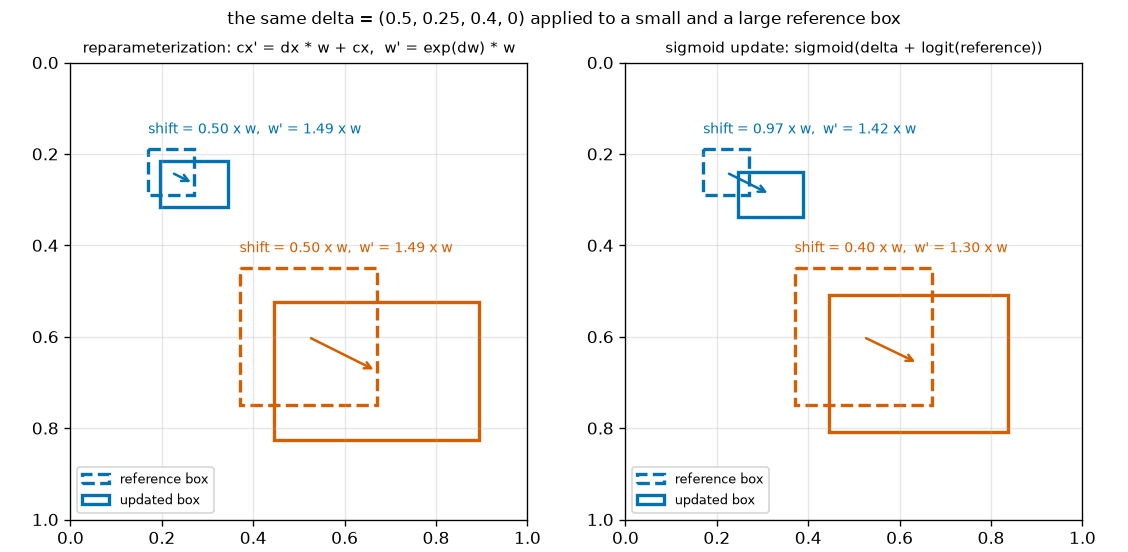
Figure 9-8 shows the same thing as the hand calculation with different deltas.
- Left (reparameterization). The labels above the two boxes are identical: "shift 0.50 times the width, width 1.49 times (\(e^{0.4} = 1.49\))". The blue and orange arrows differ in length by a factor of 3, but each is the same proportion relative to its own box. Shrink the large picture and it overlaps the small one.
- Right (chapter 8's sigmoid approach). The small box moved 0.97 times its width and the large box 0.40 times, and the width scale factors also differ, 1.42 and 1.30. The same numbers mean different things for each box.
The deltas needed in the shape world
Roughly what values must the head actually output? In the two-stage approach of chapter 8, the decoder's reference boxes started from the proposal box of each feature map cell: a small box of width · height 0.05 at the cell center. For the 501 ground-truth boxes of the shape world (200 validation images), the \(\delta\) needed to go from the proposal box of the cell containing the center to the ground truth was computed with the inverse.
  도형 세상 정답 501개를 '중심이 놓인 칸의 제안 박스 (칸 중심, 0.05, 0.05)' 에서 맞히는 데 필요한 델타
    |δx|, |δy| 최대 0.832 (반 칸 = 0.0417 / 0.05 = 0.833 이하), δw, δh 범위 1.030 – 2.127 (= log(정답 크기 / 0.05), 정답 크기 0.140 – 0.420)
- Center. On the 12×12 grid, a cell is \(1/12 = 0.0833\) wide, and a ground-truth center is at most half a cell (\(0.0417\)) from the cell center. Dividing that by the proposal box width 0.05 gives \(0.0417 / 0.05 = 0.833\). Hence \(|\delta_x|, |\delta_y| \le 0.833\).
- Size. Ground truths in the shape world have width · height between 0.14 and 0.42. \(\delta_w\) runs from \(\log(0.14 / 0.05) = \log 2.8 = 1.030\) to \(\log(0.42 / 0.05) = \log 8.4 = 2.128\): scaling the proposal box up by 2.8 to 8.4 times.
All four values are numbers around 1 in magnitude, a range a network can output comfortably. With chapter 8's approach, the same job would require adding \(\sigma^{-1}(0.42) - \sigma^{-1}(0.05) = -0.32 + 2.94 = 2.62\) in logits. Which is better for training was not tested in this tutorial. As noted above, the difference the LW-DETR paper reports on COCO is 0.2 mAP.
Mixed query selection and pretraining
Mixed query selection
The way LW-DETR's decoder obtains queries was already built in chapter 8. Section 3.1 of the paper calls it mixed-query selection, following the approach of DINO (Zhang et al., 2022; a detector that merely shares its name with the self-supervised DINO of chapter 6), and describes an object query as the sum of two parts.
- Content query: a learned embedding, as in the DETR of chapter 7. It is fixed for each query slot, independent of the image.
- Spatial query: determined by looking at the image. The \(N_q\) highest-scoring cells are picked from the projector's final output, a box is predicted from each, and the box is turned into an embedding. This is the two-stage approach of chapter 8.
"Mixed" means the two come from different sources: where to look (location) is picked from the image, and what to look for (content) is kept as a learned embedding. Chapter 8's implementation had exactly this form. The boxes of the picked cells became the decoder's reference boxes, and the query content was a learned embedding. What changes is how those boxes are handled (reparameterization) and the query groups (Group DETR); reassembling it all with RF-DETR's actual code is done in chapter 10.
Objects365 pretraining
LW-DETR's last ingredient is not structure but data. Before training on COCO, the paper pretrains on the larger detection dataset Objects365 (chapter 1). There are two stages.
- Pretraining the encoder. The ViT is pretrained on Objects365 images with a method called CAEv2, a form of self-supervised learning that masks part of the image and has the model predict it (another branch of the self-supervised learning seen in chapter 6). The paper says this gains 0.7 mAP on COCO.
- Pretraining the whole detector. While continuing to train the encoder, the projector and decoder are trained with supervision on Objects365's box labels (30 epochs). After that, the model is fine-tuned on COCO.
The effect is larger than all of this chapter's techniques combined. In table 2, the row that adds pretraining raises mAP by 8.7, from 38.6 to 47.3. The paper takes this to mean that Transformers benefit from large data. In table 5, which compares the five fully trained models, the gain from pretraining averages 5.5 mAP as well (tiny 36.5 → 42.6, xlarge 53.0 → 58.3).
The paper also reports an interesting contrast. The same Objects365 pretraining did little for the YOLO family. In table 3, YOLOv8n rises only from 37.4 to 37.6, and RTMDet-s from 44.6 to 44.9. The paper does not pin down the reason. It includes one experiment suggesting that because these detectors train for as long as 300 – 500 epochs, the pretraining gain may fade as training gets longer, and says further investigation is needed. Either way, the observation remains that the DETR family gains a lot from weights learned in advance on large data, and this is the background to RF-DETR choosing DINOv2, pretrained at internet scale, as its backbone.
Reading table 2 of the paper step by step
Here, table 2 of the LW-DETR paper, quoted piecemeal throughout this chapter, is gathered in one place. It is an ablation study that starts from a "baseline detector" using only global attention and outputting only the last layer's feature map, and stacks one technique per row until reaching the small model. Every row except the last is trained for only 45,000 steps (12 epochs). The rightmost column is the mAP difference from the row directly above; it is not in the paper's table but computed here by subtraction.
| Setting (cumulative from the top) | Params | Compute | Latency | mAP | Diff |
| Baseline detector | 10.8M | 22.8 G | 3.6 ms | 35.3 | |
| + multi-level feature aggregation | 11.0M | 23.0 G | 3.7 ms | 36.0 | +0.7 |
| + interleaved window · global attention (ViTDet-style implementation) | 11.0M | 16.6 G | 3.9 ms | 34.7 | −1.3 |
| + window-major organization | 11.0M | 16.6 G | 2.9 ms | 34.7 | 0 |
| + IoU-aware classification loss (IA-BCE) | 11.0M | 16.6 G | 2.9 ms | 35.4 | +0.7 |
| + more supervision (Group DETR) | 14.6M | 16.6 G | 2.9 ms | 38.4 | +3.0 |
| + box reparameterization | 14.6M | 16.6 G | 2.9 ms | 38.6 | +0.2 |
| + Objects365 pretraining | 14.6M | 16.6 G | 2.9 ms | 47.3 | +8.7 |
| LW-DETR-small (trained to 180,000 steps) | 14.6M | 16.6 G | 2.9 ms | 48.0 | +0.7 |
Read the table step by step, going down one row at a time.
- Only two rows change speed: window attention (compute 23.0 → 16.6 GFLOPs) and window-major organization (latency 3.9 → 2.9 ms). In the five rows below them, compute and latency never change. IA-BCE, Group DETR, reparameterization, and pretraining are all training methods and do not touch the computation at inference.
- Window attention is paid for in accuracy. It gave up 1.3 mAP to gain 0.8 ms of latency (3.7 → 2.9). The training techniques right below it more than make up for that loss. "Make the structure fast, recover accuracy through training" is LW-DETR's design.
- The two biggest steps are supervision and data. Group DETR gives +3.0 and pretraining +8.7. Together, these two rows' 11.7 make up most of the 12.7 mAP gained from the baseline detector to the final model.
- Group DETR is the only row that adds parameters (11.0M → 14.6M). As seen above, this is the per-group query embeddings and query selection heads, which are not used at inference.
- Reading a cumulative ablation
- The "diff" in such a table is not the worth of that technique but its increment when stacked in that order. Changing the order could change it. For example, had pretraining been added first and Group DETR afterward, the gain might have been smaller or larger than +3.0; the paper does not include that experiment. Nor is there any guarantee that a difference seen in 12-epoch training holds when training runs to completion. Techniques that speed up convergence, like Group DETR, look especially large in short training.
Reading the implementation
Most of the per-part code has already been shown. Here we look at how to run the whole practice file, and read the code not yet opened: the windowed ViT encoder, the projector, and per-group matching. The mini RF-DETR in chapter 10 reuses the parts in this file as they are.
Running it
$ python ch09_lwdetr_parts.py            # 본문의 결과 (노트북 GPU 에서 약 32초)
$ python ch09_lwdetr_parts.py --quick    # 줄인 판 (CPU 에서 약 7초)
This file does no training. For each part it prints a hand-calculated example, checks values against PyTorch built-in operations, and draws five figures. Most of the time goes to timing window attention (48×48 grid, three approaches × 40 rounds). --quick only reduces the number of timing rounds and the grid size. The execution order is as follows, and the last two lines of output are shown below.
def main():
    parser = argparse.ArgumentParser()
    parser.add_argument("--quick", action="store_true")
    parser.add_argument("--fig-dir", default="figures")
    parser.add_argument("--seed", type=int, default=0)
    args = parser.parse_args()
    import matplotlib
    matplotlib.use("Agg")
    os.makedirs(args.fig_dir, exist_ok=True)
    torch.manual_seed(args.seed)
    device = get_device()
    if device == "cpu":
        torch.set_num_threads(4)
    start = time.time()
    print(f"장치: {device}")

    toy_window_order()
    pair_rows, time_rows = window_checks(device, args.quick)
    vit = vit_checks()
    projector_checks(vit)
    ia_bce_checks()
    group_checks()
    reparam_checks()

    plot_window_order(os.path.join(args.fig_dir, "ch09-window-order.png"))
    plot_window_cost(pair_rows, time_rows, device, os.path.join(args.fig_dir, "ch09-window-cost.png"))
    shares = plot_influence(os.path.join(args.fig_dir, "ch09-window-influence.png"))
    print("[그림 ch09-window-influence] 출력 칸 (행 2, 열 3) 이 받는 영향 가운데 자기 윈도 안 패치의 몫: "
          f"윈도 블록만 {shares[0]:.3f}, 윈도 + 전역 {shares[1]:.3f}, 전역만 {shares[2]:.3f}")
    plot_ia_bce(os.path.join(args.fig_dir, "ch09-ia-bce.png"))
    plot_reparam(os.path.join(args.fig_dir, "ch09-reparam.png"))
    print(f"그림 5장 저장: {args.fig_dir}/ch09-*.png  |  전체 {time.time() - start:.1f}초")
[그림 ch09-window-influence] 출력 칸 (행 2, 열 3) 이 받는 영향 가운데 자기 윈도 안 패치의 몫: 윈도 블록만 1.000, 윈도 + 전역 0.910, 전역만 0.838
그림 5장 저장: /home/zer0/Projects/pages/public/rf-detr/figures/ch09-*.png  |  전체 32.1초
Windowed ViT encoder
Start the encoder with its blocks. SelfAttention is the multi-head self-attention of chapter 5 as is, and ViTBlock is the pre-norm block of chapter 6 with one extra argument, merge. With merge=1, attention runs on the incoming shape as is (in window-major organization, this is window attention); with merge=m, the \(m\) adjacent rows of the batch are joined into one row with view, attention is run, and the shape is restored (global attention). Note that the difference between window attention and global attention has shrunk to two reshape lines. The MLP after attention is computed per token, so it gives the same result whichever shape it is fed.
class SelfAttention(nn.Module):
    """다중 머리 자기 어텐션 (5장). 입력 (B, T, C) 의 토큰 T 개가 서로를 본다 — 배치의 다른 줄은 보지 않는다.

    "윈도 어텐션" 을 위한 특별한 코드는 없다. 윈도를 배치 축에 올려 (B·윈도 수, 윈도 안 토큰 수, C) 로 넣으면
    이 모듈이 저절로 윈도 안에서만 어텐션을 한다.
    """

    def __init__(self, dim: int, heads: int):
        super().__init__()
        assert dim % heads == 0
        self.heads = heads
        self.qkv = nn.Linear(dim, 3 * dim)  # 질의 · 열쇠 · 값 투영을 한 번에
        self.proj = nn.Linear(dim, dim)

    def forward(self, x: torch.Tensor) -> torch.Tensor:
        batch, tokens, dim = x.shape
        qkv = self.qkv(x).view(batch, tokens, 3, self.heads, dim // self.heads).permute(2, 0, 3, 1, 4)
        q, k, v = qkv[0], qkv[1], qkv[2]  # 각각 (B, 머리, T, C/머리)
        out = F.scaled_dot_product_attention(q, k, v)  # softmax(QKᵀ/√d)·V — 계산량이 T² 에 비례한다
        return self.proj(out.transpose(1, 2).reshape(batch, tokens, dim))

class ViTBlock(nn.Module):
    """ViT 블록 한 개 (pre-norm): x + γ₁·어텐션(LN(x)), 이어서 x + γ₂·MLP(LN(x)).

    DINOv2 처럼 잔차 가지마다 학습되는 배율 γ (LayerScale) 가 있다. merge 인자가 윈도 · 전역을 가른다.
    """

    def __init__(self, dim: int, heads: int, mlp_ratio: float = 4.0, layer_scale: float = 1.0):
        super().__init__()
        self.norm1 = nn.LayerNorm(dim, eps=1e-6)
        self.attn = SelfAttention(dim, heads)
        self.gamma1 = nn.Parameter(torch.full((dim,), layer_scale))
        self.norm2 = nn.LayerNorm(dim, eps=1e-6)
        hidden = int(dim * mlp_ratio)
        self.mlp = nn.Sequential(nn.Linear(dim, hidden), nn.GELU(), nn.Linear(hidden, dim))
        self.gamma2 = nn.Parameter(torch.full((dim,), layer_scale))

    def forward(self, x: torch.Tensor, merge: int = 1) -> torch.Tensor:
        """x: (B', T, C).  merge = 1 이면 들어온 모양 그대로 어텐션 (윈도 우선 배치에서는 "윈도 어텐션").

        merge = m > 1 이면 배치의 이웃한 m 줄을 한 줄로 이어 붙여 (B'/m, m·T, C) 로 보고 어텐션을 한 뒤 되돌린다.
        윈도 우선 배치에서 m = 윈도 수면 "전역 어텐션" 이다. 메모리에서 이웃한 줄을 붙이는 것이라 view 만으로 된다
        (값을 옮기지 않는다) — 이것이 윈도 우선 배치의 이득이다.
        """
        shape = x.shape
        y = self.norm1(x)
        if merge > 1:
            y = y.view(shape[0] // merge, merge * shape[1], shape[2])
        y = self.attn(y).view(shape)
        x = x + self.gamma1 * y
        return x + self.gamma2 * self.mlp(self.norm2(x))
gamma1 · gamma2, multiplied into each residual branch, are the learned scales (LayerScale) in DINOv2's blocks. They were added to match the form of RF-DETR's backbone; their initial value is 1, so at first they have no effect.
Which blocks use windows is decided by a function that ports the public implementation's rule as is.
def compute_window_block_indexes(out_feature_indexes, window_block_indexes=None):
    """어느 블록이 윈도 어텐션을 쓰는가 (0 부터 센 블록 번호의 목록). 공식 구현의 규칙 그대로다.

    따로 지정하지 않으면 0 … out_feature_indexes[-1] 가운데 out_feature_indexes 에 **없는** 번호가 윈도 블록이다.
    예: [3, 6, 9, 12] → 윈도 [0, 1, 2, 4, 5, 7, 8, 10, 11], 전역은 블록 3, 6, 9.
    out_feature_indexes 의 숫자 i 는 "블록 i 개를 지난 뒤의 특징" 이라는 뜻이므로 (0 = 임베딩 직후),
    특징을 꺼낸 **바로 다음** 블록이 전역 블록이 된다.
    """
    if window_block_indexes is not None:
        return sorted(window_block_indexes)
    return sorted(set(range(out_feature_indexes[-1] + 1)) - set(out_feature_indexes))
The rule is "blocks that are not feature-map extraction points are window blocks". A number \(i\) in out_feature_indexes means "the features after passing \(i\) blocks" (0 is right after the embedding). The mini model uses (2, 4, 6), so of 0 – 6, removing 2, 4, 6 leaves blocks 0, 1, 3, 5 as window blocks, and blocks 2, 4 are global (6 falls outside the block index range 0 – 5, so no block corresponds to it). The pattern is that the block right after a feature extraction point becomes a global block. Plugging in RF-DETR Nano's setting [3, 6, 9, 12], blocks 3, 6, 9 of the 12 are global and the other 9 are window blocks. That the window block indices given in the paper's appendix differ from this behavior of the public code is discussed in chapter 10.
(The code of the windowed-vit region, collapsed in the original, is in ch09_lwdetr_parts.py.)
Follow the five steps of WindowedViT.forward through tensor shapes (2 images, 96×96, patch 8, dimension 96, 2×2 windows).
[WindowedViT] 기본 설정: 그림 96, 패치 8, 차원 96, 블록 6, 머리 4, 꺼내는 층 [2, 4, 6], 윈도 2×2
  윈도 블록 [0, 1, 3, 5], 전역 블록 [2, 4], 매개변수 705,024개
  공식 규칙 확인: compute_window_block_indexes([3, 6, 9, 12]) = [0, 1, 2, 4, 5, 7, 8, 10, 11]
  모양 추적 (B = 2)
    그림                         (2, 3, 96, 96)
    패치 임베딩 + CLS + 위치      (2, 145, 96)   (1 + 12·12 토큰)
    윈도 우선 재배열 (패치만)     (8, 36, 96)    (B·4 윈도, 6·6 토큰)
    윈도마다 CLS 를 붙인 뒤       (8, 37, 96)    ← 윈도 블록의 입력
    전역 블록 안에서의 view       (2, 148, 96)   (4·37 토큰: CLS 4개 포함)
    꺼낸 특징 맵 3개              각각 (2, 96, 12, 12)
- Patch embedding. An 8×8 convolution (stride 8) produces 12×12 = 144 patch tokens; a CLS token is prepended and learned position embeddings are added.
(2, 145, 96). - Window-major reordering. Only the 144 patch tokens are rearranged with
to_window_major. The 4 windows move onto the batch axis:(8, 36, 96). - CLS token duplication. The CLS token, with its position embedding already added, is duplicated once per window and prepended. Each window has 1 + 36 = 37 tokens,
(8, 37, 96). This is the input to the window blocks. - Global blocks. Joining the 4 windows into one row with
viewgives 4 × 37 = 148 tokens. The 144 patch tokens are mixed with 4 CLS tokens, and in global attention these 4 CLS tokens also see each other. - Taking out the feature maps. At each designated layer, apply layer normalization, drop the CLS tokens, restore row-major order with
from_window_major, and fold into(2, 96, 12, 12). The order is restored only when taking features out.
Because of the CLS tokens, the attention pairs are a little more than in the earlier calculation. Window blocks have \(4 \times 37^2 = 5{,}476\) pairs (5,184 with patches only), and global blocks \(148^2 = 21{,}904\) pairs (20,736 with patches only). Keep in mind that the more windows there are, the more CLS tokens get duplicated. This comes up again in chapter 10, where RF-DETR chooses the number of windows.
This encoder was built so that input resolution, patch size, and number of windows can be changed on each call while keeping the weights as they are. The NAS of chapter 12 turns these knobs.
  손잡이 (가중치는 그대로, 호출 인자만 바꿈)
    해상도  96, 패치  8, 윈도 2×2 → 특징 맵 (1, 96, 12, 12)
    해상도  96, 패치  8, 윈도 1×1 → 특징 맵 (1, 96, 12, 12)
    해상도  96, 패치  8, 윈도 3×3 → 특징 맵 (1, 96, 12, 12)
    해상도  64, 패치  8, 윈도 2×2 → 특징 맵 (1, 96, 8, 8) (위치 임베딩 보간)
    해상도 128, 패치  8, 윈도 2×2 → 특징 맵 (1, 96, 16, 16) (위치 임베딩 보간)
    해상도  96, 패치 12, 윈도 2×2 → 특징 맵 (1, 96, 8, 8) (위치 임베딩 보간) (패치 임베딩 보간)
    해상도  96, 패치  6, 윈도 2×2 → 특징 맵 (1, 96, 16, 16) (위치 임베딩 보간) (패치 임베딩 보간)
    해상도  96, 패치 16, 윈도 1×1 → 특징 맵 (1, 96, 6, 6) (위치 임베딩 보간) (패치 임베딩 보간)
The number of windows only changes how attention is grouped, so the parameters do not change at all (the first three lines). Changing the resolution or patch size changes the grid size, so the position embeddings are interpolated (chapter 6). There are two constraints: each side of the image must be a multiple of the patch size, and each side of the grid must be a multiple of the number of windows. For a 12×12 grid, the number of windows per side can be 1, 2, 3, 4, or 6.
def resize_patch_embed_simple(weight: torch.Tensor, new_patch: int) -> torch.Tensor:
    """패치 임베딩 합성곱의 가중치를 다른 패치 크기로 바꾸는 가장 단순한 방법: 가중치를 그림처럼 보간한다.

    weight: (C, 3, p, p) → (C, 3, p', p').  쌍삼차 보간 뒤 (p/p')² 를 곱해, 밋밋한 패치에 대한 응답 크기를 맞춘다
    (가중치의 합이 p'²/p² 배로 늘어나는 것을 되돌린다).
    FlexiViT 는 이보다 나은 변환(보간의 유사 역행렬)을 쓴다 — 12장에서 WindowedViT.patch_resize_fn 에 끼워 넣는다.
    """
    old_patch = weight.shape[-1]
    if new_patch == old_patch:
        return weight
    resized = F.interpolate(weight, size=(new_patch, new_patch), mode="bicubic", align_corners=False, antialias=True)
    return resized * (old_patch / new_patch) ** 2
- What this output does and does not say
- The table above shows only that the shapes work out. The model is untrained, and the accuracy under changed settings was not measured. In particular,
resize_patch_embed_simple, which changes the patch size, is the simplest method: it interpolates the patch embedding weights like an image. It is not the FlexiViT-style transform the RF-DETR paper says it uses. Comparing against that transform and its accuracy is left to chapter 12.
Projector code
The projector has four parts: ChannelLayerNorm, which normalizes the channel axis; ConvX, the "convolution → normalization → activation function" bundle; Bottleneck, two 3×3 ConvX; and C2f. The three lines of C2f.forward are figure 9-5 as is: split the output of cv1 in two with split, repeatedly feed the last element of the list into a bottleneck and append the result to the list, then join the whole list with cat and feed it to cv2.
class ChannelLayerNorm(nn.Module):
    """(B, C, H, W) 특징 맵용 층 정규화: 칸마다 채널 C 개에 걸쳐 평균 0 · 분산 1 로 맞춘다.

    nn.LayerNorm 은 마지막 축을 정규화하므로, 채널 축을 맨 뒤로 보냈다가 되돌린다.
    배치 정규화와 달리 배치의 다른 그림을 보지 않는다 → 배치가 작아도 (기울기 누적을 써도) 동작이 같다.
    """

    def __init__(self, channels: int, eps: float = 1e-6):
        super().__init__()
        self.weight = nn.Parameter(torch.ones(channels))
        self.bias = nn.Parameter(torch.zeros(channels))
        self.eps = eps

    def forward(self, x: torch.Tensor) -> torch.Tensor:
        x = F.layer_norm(x.permute(0, 2, 3, 1), self.weight.shape, self.weight, self.bias, self.eps)
        return x.permute(0, 3, 1, 2)

class ConvX(nn.Module):
    """합성곱(편향 없음) → 정규화 → 활성 함수. layer_norm=True 면 층 정규화(RF-DETR), False 면 배치 정규화(LW-DETR)."""

    def __init__(self, cin: int, cout: int, kernel: int = 3, stride: int = 1, act: str = "relu",
                 layer_norm: bool = True):
        super().__init__()
        self.conv = nn.Conv2d(cin, cout, kernel, stride, padding=kernel // 2, bias=False)
        self.bn = ChannelLayerNorm(cout) if layer_norm else nn.BatchNorm2d(cout)  # 이름은 공식 구현을 따라 bn
        self.act = nn.SiLU() if act == "silu" else nn.ReLU()

    def forward(self, x: torch.Tensor) -> torch.Tensor:
        return self.act(self.bn(self.conv(x)))

class Bottleneck(nn.Module):
    """3×3 ConvX 두 번. shortcut=True 이고 채널 수가 같으면 입력을 더한다 (C2f 안에서는 기본이 False)."""

    def __init__(self, c1: int, c2: int, shortcut: bool = True, e: float = 0.5, act: str = "silu",
                 layer_norm: bool = True):
        super().__init__()
        hidden = int(c2 * e)
        self.cv1 = ConvX(c1, hidden, 3, act=act, layer_norm=layer_norm)
        self.cv2 = ConvX(hidden, c2, 3, act=act, layer_norm=layer_norm)
        self.add = shortcut and c1 == c2

    def forward(self, x: torch.Tensor) -> torch.Tensor:
        return x + self.cv2(self.cv1(x)) if self.add else self.cv2(self.cv1(x))

class C2f(nn.Module):
    """C2f 블록 (YOLOv8). 입력 (B, c1, H, W) → 출력 (B, c2, H, W), 해상도는 그대로.

    1) 1×1 ConvX 로 2c 채널 (c = c2/2) → 반씩 둘로 나눈다: y₀, y₁
    2) 병목 n 개를 차례로: y₂ = m₁(y₁), y₃ = m₂(y₂), …
    3) y₀ … y_{n+1} 을 모두 채널 방향으로 이어 붙여 ((2 + n)·c 채널) 1×1 ConvX 로 c2 채널
    중간 결과를 전부 마지막에 모으므로, 얕은 경로와 깊은 경로의 특징이 함께 쓰인다.
    """

    def __init__(self, c1: int, c2: int, n: int = 1, shortcut: bool = False, e: float = 0.5, act: str = "silu",
                 layer_norm: bool = True):
        super().__init__()
        self.c = int(c2 * e)
        self.cv1 = ConvX(c1, 2 * self.c, 1, act=act, layer_norm=layer_norm)
        self.cv2 = ConvX((2 + n) * self.c, c2, 1, act=act, layer_norm=layer_norm)
        self.m = nn.ModuleList(Bottleneck(self.c, self.c, shortcut, e=1.0, act=act, layer_norm=layer_norm)
                               for _ in range(n))

    def forward(self, x: torch.Tensor) -> torch.Tensor:
        y = list(self.cv1(x).split((self.c, self.c), dim=1))
        y.extend(m(y[-1]) for m in self.m)
        return self.cv2(torch.cat(y, dim=1))
MultiScaleProjector builds one stage per scale factor: "(resize each input) → concatenate along channels → C2f → layer normalization". That its input is a list of feature maps from several layers is the implementation of multi-level feature aggregation: the single line torch.cat([...], dim=1) in forward.
SCALE_FACTORS = {"P3": 2.0, "P4": 1.0, "P5": 0.5}  # ViT 특징 맵(P4) 기준의 배율

class MultiScaleProjector(nn.Module):
    """ViT 의 여러 층 특징 맵을 받아 디코더가 읽을 특징 맵(들)을 만든다 (공식 projector.py 와 같은 구조).

    입력: 목록 [(B, C_j, h, w), …] — 모두 같은 해상도 (ViT 는 층이 달라도 해상도가 같다).
    scale_factors 의 배율마다 한 단계(stage)씩:
      배율 2.0 (P3): 입력마다 전치 합성곱(2×2, 스트라이드 2)으로 2배 키우고 채널은 절반
      배율 1.0 (P4): 그대로
      배율 0.5 (P5): 입력마다 3×3 스트라이드 2 ConvX 로 절반
      → 입력들을 채널 방향으로 이어 붙임 → C2f(num_blocks) → 층 정규화
    돌려주는 값: 목록 [(B, out_channels, h·배율, w·배율), …]  (배율 순서대로).
    RF-DETR 의 기본은 P4 한 단계뿐이다 (단일 스케일).
    """

    def __init__(self, in_channels, out_channels: int, scale_factors=(1.0,), num_blocks: int = 3,
                 layer_norm: bool = True):
        super().__init__()
        self.scale_factors = list(scale_factors)
        sampling, stages = [], []
        for scale in self.scale_factors:
            layers = []
            for cin in in_channels:
                if scale == 2.0:
                    layers.append(nn.Sequential(nn.ConvTranspose2d(cin, cin // 2, kernel_size=2, stride=2)))
                elif scale == 1.0:
                    layers.append(nn.Sequential())
                elif scale == 0.5:
                    layers.append(nn.Sequential(ConvX(cin, cin, 3, 2, layer_norm=layer_norm)))
                else:
                    raise NotImplementedError(f"지원하지 않는 배율: {scale}")
            sampling.append(nn.ModuleList(layers))
            fused = sum(cin // 2 if scale == 2.0 else cin for cin in in_channels)
            stages.append(nn.Sequential(C2f(fused, out_channels, num_blocks, layer_norm=layer_norm),
                                        ChannelLayerNorm(out_channels)))
        self.stages_sampling = nn.ModuleList(sampling)
        self.stages = nn.ModuleList(stages)

    def forward(self, features):
        results = []
        for sampling, stage in zip(self.stages_sampling, self.stages):
            fused = torch.cat([layer(x) for layer, x in zip(sampling, features)], dim=1)  # 여러 층을 채널로 잇는다
            results.append(stage(fused))
        return results
Per-group matching code
GroupHungarianMatcher inherits chapter 7's HungarianMatcher (with chapter 8's focal-form classification cost) and changes only two things. assign_groups cuts the cost matrix by group and solves the Hungarian problem separately for each, and cost_parts computes the L1 cost by subtraction instead of torch.cdist (the values are the same, and it is faster for the small matrices called at every training step). The matching cost weights are RF-DETR's defaults: classification 2, L1 5, GIoU 2. The training in chapter 11 uses this class.
class GroupHungarianMatcher(HungarianMatcher):
    """묶음마다 따로 하는 헝가리안 매칭. 7장 HungarianMatcher (포컬 꼴 비용) 에 묶음 나누기만 더했다.

    예측 G·N 개를 N 개씩 G 묶음으로 나누고, 묶음마다 그림의 정답 전체와 일대일 매칭을 푼다.
    → 정답 하나가 묶음마다 한 번씩, 모두 G 번 짝을 얻는다 (학습 신호가 G 배). 추론 때는 묶음이 하나뿐이다.
    """

    def __init__(self, cost_class: float = 2.0, cost_bbox: float = 5.0, cost_giou: float = 2.0):
        super().__init__(cost_class, cost_bbox, cost_giou, class_cost="focal")

    @torch.no_grad()
    def cost_parts(self, logits, boxes, tgt_labels, tgt_boxes):
        """7장과 같은 세 비용 (포컬 꼴 분류 비용, L1, −GIoU), 각각 (Q, T). L1 만 torch.cdist 대신 뺄셈으로 계산한다

        (값은 같고, 이렇게 작은 행렬에서는 GPU 에서 훨씬 빠르다 — 학습 스텝마다 불리므로 차이가 쌓인다).
        """
        prob = logits.sigmoid()[:, tgt_labels]  # (Q, T): 열 j 는 정답 j 의 클래스에 준 확률
        alpha, gamma = self.focal_alpha, self.focal_gamma
        c_cls = (alpha * (1 - prob) ** gamma * (-(prob + 1e-8).log())
                 - (1 - alpha) * prob**gamma * (-(1 - prob + 1e-8).log()))
        c_l1 = (boxes[:, None] - tgt_boxes[None]).abs().sum(-1)
        c_giou = -generalized_box_iou(box_cxcywh_to_xyxy(boxes), box_cxcywh_to_xyxy(tgt_boxes))
        return c_cls, c_l1, c_giou

    @staticmethod
    def assign_groups(cost: np.ndarray, group_detr: int):
        """그림 한 장의 비용 행렬 (G·N, T) 을 묶음별로 잘라 각각 헝가리안 풀이를 한다.

        돌려주는 값: (예측 번호 (G·T,), 정답 번호 (G·T,)) — 예측 번호는 0 … G·N−1.
        """
        per_group = cost.shape[0] // group_detr
        rows, cols = [], []
        for g in range(group_detr):
            r, c = linear_sum_assignment(cost[g * per_group:(g + 1) * per_group])  # 묶음 g 안에서만 푼다
            rows.append(r + g * per_group)
            cols.append(c)
        return np.concatenate(rows), np.concatenate(cols)

    @torch.no_grad()
    def forward(self, outputs, targets, group_detr: int = 1):
        """outputs: {"pred_logits": (B, G·N, K), "pred_boxes": (B, G·N, 4)}.

        돌려주는 값: 길이 B 의 목록. b 번째는 (pred_idx, tgt_idx) — 길이 G·T_b. pred_idx 는 0 … G·N−1 의 번호.
        """
        batch, total = outputs["pred_logits"].shape[:2]
        sizes = [len(t["labels"]) for t in targets]
        cost = self.cost_matrix(
            outputs["pred_logits"].flatten(0, 1), outputs["pred_boxes"].flatten(0, 1),
            torch.cat([t["labels"] for t in targets]), torch.cat([t["boxes"] for t in targets]),
        ).view(batch, total, -1).cpu().numpy()  # (B, G·N, ΣT)
        offsets = np.cumsum([0] + sizes)
        indices = []
        for b in range(batch):  # block: (G·N, T_b) — 이 그림의 예측 × 이 그림의 정답
            rows, cols = self.assign_groups(cost[b, :, offsets[b]:offsets[b + 1]], group_detr)
            indices.append((torch.as_tensor(rows, dtype=torch.long), torch.as_tensor(cols, dtype=torch.long)))
        return indices
- Comparison with the official implementation
- The parts in this chapter were checked against the corresponding modules of the installed
rfdetrpackage (1.12.1), with the same inputs and the same weights (the comparison script is not included in the practice file). The windowed ViT encoder's feature maps, the result ofcompute_window_block_indexes, and the per-group matching assignments matched the official implementation; the projector output had a maximum difference of \(10^{-5}\), and the IA-BCE loss value was the same, 6.831939. The patch-size-changing path has no counterpart in the official implementation and could not be compared. Also, LW-DETR's official repository was not examined; statements that something is "the same as LW-DETR" were verified against the paper and RF-DETR's code, which inherits from it.
From LW-DETR to RF-DETR
The RF-DETR paper introduces its architecture as "a modernized LW-DETR". Most of the parts learned in this chapter carry over as they are, and a few change. Before moving on to chapter 10, here is a map.
| Part | LW-DETR | RF-DETR | Covered in |
| Skeleton | ViT encoder → projector → deformable cross-attention decoder | Unchanged | Chapter 10 |
| Backbone | ViT pretrained with CAEv2 (10 layers, no CLS token) | DINOv2 (12 layers, has a CLS token → duplicated per window) | Chapters 6, 10 |
| Window · global attention, window-major organization | 16 windows (4 per side) | Used as is, but the number of windows becomes a knob (usually 2 per side) | Chapters 10, 12 |
| Multi-level feature aggregation · C2f projector | Batch normalization | Layer normalization | Chapter 4, this chapter |
| Decoder | Fixed at 3 layers | Loss on every layer, and layers can be dropped at inference | Chapters 10, 12 |
| Mixed query selection | Used | Unchanged | Chapters 8, 10 |
| IA-BCE · Group DETR (13 groups) · box reparameterization | Used | Unchanged (defaults in the public code) | This chapter, chapter 11 |
| Objects365 pretraining | Used | Used (backbone starts from DINOv2) | Chapter 11 |
| How model sizes are chosen | Five hand-designed sizes | Searched with weight-sharing NAS | Chapter 12 |
| Instance segmentation | None | Adds a lightweight segmentation head | Chapter 13 |
The changes all point in one direction. LW-DETR built a real-time DETR that beats YOLO on COCO, and RF-DETR pushes that architecture toward a large pretrained backbone and knobs that can be turned without retraining. The ablation in table 5 of the RF-DETR paper starts from LW-DETR (M) at 52.6 AP and, through the DINOv2 backbone, additional pretraining, and NAS, reaches 54.6 AP. The switch to layer normalization, the duplication of the CLS token, and the design that lets decoder layers be dropped are all adjustments needed along that path.
Summary
- Two paths to real time. RT-DETR redesigned the encoder after the CNN backbone to be lighter (attention only on the coarsest feature map, cross-scale fusion by convolution), and LW-DETR used a plain ViT as the encoder. Neither has NMS, so network time is total time.
- LW-DETR's structure. ViT encoder (interleaved window · global attention, gathering feature maps from several layers) → C2f projector → 3-layer decoder (deformable cross-attention) + mixed query selection. Cutting the decoder from 6 to 3 layers takes it from 1.4 to 0.7 ms.
- Window attention. Moving windows onto the batch axis turns ordinary self-attention into window attention. The pair count drops from \(N^2\) to \(N^2 / W_n^2\), but only the quadratic term shrinks, so with few tokens there is no speed gain. Without global blocks, no information at all flows between windows.
- Window-major organization. Laying out tokens window by window lets both window blocks and global blocks work with
viewalone. The paper reported 3.9 → 2.9 ms from this; in this tutorial's PyTorch measurements, no difference was measured. - C2f. 1×1 convolution → split in two → bottlenecks (two 3×3 each) in sequence → concatenate all intermediate results and apply a 1×1 convolution. With input 288 · output 128 · 3 bottlenecks, it has 300,544 parameters.
- IA-BCE. BCE with positive-cell target \(t = p^{0.25} u^{0.75}\), and BCE multiplied by \(p^2\) for negative cells. The positive-cell gradient \(p - t\) is zero at \(p = u\), so the score is pulled toward the IoU.
- Group DETR. \(G\) query groups share the decoder and are matched one-to-one separately, so there are \(G\) times as many positives. Groups do not see each other in self-attention, and inference uses only the first group, so inference cost does not increase.
- Box reparameterization. \(\hat{x} = \delta_x w_r + x_r\), \(\hat{w} = e^{\delta_w} w_r\). The deltas are measured in units of the reference box's size, so they mean the same thing regardless of box size, and with \(\delta = 0\) the reference box is unchanged.
- The paper's ablation. In LW-DETR's table 2, the biggest steps are Objects365 pretraining (+8.7) and Group DETR (+3.0). Only window attention and window-major organization change speed; the rest are training techniques with no inference cost.
The ingredients that made the DETR family real-time are now gathered: window attention and window-major organization in the encoder, the C2f projector mixing features from several layers between the encoder and decoder, and IA-BCE, Group DETR, and box reparameterization for training. In this chapter the parts were built and checked one at a time. In chapter 10, they are joined with the deformable attention decoder of chapter 8 to assemble a complete RF-DETR. The places where it differs from LW-DETR are examined there: the DINOv2 backbone and the CLS token duplicated per window, the actual code for two-stage query selection, the lightweight refinement that does not replace reference boxes at every layer, and the knobs turned without retraining.
Review questions
- 1. Counting window attention pairs — RF-DETR Nano cuts a 384×384 image into 16×16 patches and makes windows by splitting each side in 2. Answer without the CLS token. (a) What is the number of tokens \(N\), and the number of pairs in one global attention pass? (b) What is the number of tokens per window, and the number of pairs in one window attention pass? (c) If 3 of 12 blocks are global and 9 are window blocks, how many times the all-global case are the attention pairs across the whole encoder?
- (a) \(384 / 16 = 24\) per side, so \(N = 24^2 = 576\). Global attention has \(576^2 = 331{,}776\) pairs.
- (b) There are \(2 \times 2 = 4\) windows, with \(576 / 4 = 144\) tokens each (12×12). The pairs are \(4 \times 144^2 = 4 \times 20{,}736 = 82{,}944\), the same as the formula \(N^2 / W_n^2 = 331{,}776 / 4\).
- (c) \((3 \times 1 + 9 \times \tfrac{1}{4}) / 12 = 5.25 / 12 = 0.4375\) times. All 9 window layers together amount to 2.25 global layers. This counts only attention pairs; the linear layers and MLPs do not shrink, so the compute of the whole blocks drops less than this.
- 2. Window-major positions — In the text's 4×4 grid · 2×2 window example, (a) which cell is at window-major position \(k = 13\)? (b) At which position in window-major order does cell \(f_{23}\) land? Use \(k = 8a + 4b + 2i + j\) and the row-major index \(8a + 4i + 2b + j\).
- (a) \(13 = 8 \cdot 1 + 4 \cdot 1 + 2 \cdot 0 + 1\), so \((a, b, i, j) = (1, 1, 0, 1)\). The row-major index is \(8 \cdot 1 + 4 \cdot 0 + 2 \cdot 1 + 1 = 11\), that is, \(r = 2\), \(c = 3\), so it is \(f_{34}\). This matches the value 11 at position 13 in the list printed in the text.
- (b) \(f_{23}\) has \(r = 1\), \(c = 2\), so \(a = 0, i = 1, b = 1, j = 0\). Its window-major position is \(k = 8 \cdot 0 + 4 \cdot 1 + 2 \cdot 1 + 0 = 6\). Its row-major index is also \(4 \cdot 1 + 2 = 6\), so this cell has the same position in both layouts. It is the third cell of the top-right window.
- 3. Less compute, not less time — In this chapter's measurements, on the 12×12 grid window attention cut the pairs to a quarter, yet the time stayed almost the same, from 1.01 ms to 0.97 ms. On the 48×48 grid it became 0.59 times. Explain this difference using chapter 6's estimate \(12ND^2 + 2N^2D\) (\(D = 96\)). And what reason did the LW-DETR paper give for latency rising while compute fell?
- Window attention reduces only the quadratic term \(2N^2D\). The ratio of the two terms is \(N / 6D\), which on the 12×12 grid (\(N = 144\)) is \(144 / 576 = 0.25\). Attention pairs account for only \(0.25 / 1.25 = 20\%\) of a block's compute, so cutting them to a quarter reduces one block by only 15%, and since only 4 of the 6 blocks are window blocks, the total drops by 10%. For a computation this small, even that 10% is buried under call overhead.
- On the 48×48 grid (\(N = 2304\)), \(N / 6D = 4\), so attention pairs are 80% of a block. A window block becomes \((1 + 1)/(1 + 4) = 0.4\) times, and the total \((2 \times 5 + 4 \times 2) / (6 \times 5) = 0.60\) times, matching the measured 0.59.
- The reason the paper gives is the reordering (moving values in memory) required for every window block with row-major order. Compute (FLOPs) counts only multiplications and additions, so such costs do not show up. Window-major organization eliminates that reordering.
- 4. Channels and parameters of C2f — There is a C2f block with 192 input channels, 64 output channels, and 2 bottlenecks (layer normalization, no bias in the convolutions). (a) What is \(c\), and how many channels go into the final 1×1 convolution? (b) How many parameters does the C2f block have?
- (a) \(c = 64 / 2 = 32\). There are four branches to concatenate, \(y_0, y_1, y_2, y_3\), so \((2 + 2) \times 32 = 128\) channels.
- (b) cv1: \(192 \times 64 + 2 \times 64 = 12{,}288 + 128 = 12{,}416\). One 3×3 ConvX: \(32 \times 32 \times 9 + 2 \times 32 = 9{,}216 + 64 = 9{,}280\); there are four in the 2 bottlenecks, so \(37{,}120\). cv2: \(128 \times 64 + 2 \times 64 = 8{,}192 + 128 = 8{,}320\). The total is \(12{,}416 + 37{,}120 + 8{,}320 = 57{,}856\).
- 5. IA-BCE by hand — A prediction matched to a ground truth has score \(p = 0.70\) and box IoU \(u = 0.60\) (\(\alpha = 0.25\)). Use \(0.70^{0.25} = 0.9147\), \(0.60^{0.75} = 0.6817\), \(\log 0.7 = -0.3567\), \(\log 0.3 = -1.2040\). (a) What is the target \(t\)? (b) What is this cell's loss? (c) What is the gradient with respect to the logit, and what does it mean? (d) What would the loss and gradient be with ordinary BCE (target 1)?
- (a) \(t = 0.9147 \times 0.6817 = 0.6236\). It lies between \(u = 0.60\) and \(p = 0.70\).
- (b) \(-0.6236 \times (-0.3567) - 0.3764 \times (-1.2040) = 0.2224 + 0.4532 = 0.6756\).
- (c) \(p - t = 0.70 - 0.6236 = +0.0764\). It is positive, so gradient descent lowers the logit. The score is above the IoU, so the signal is to lower it.
- (d) Loss \(-\log 0.7 = 0.3567\), gradient \(0.70 - 1 = -0.30\). A signal to raise the score further, regardless of how well the box fits.
- 6. The exponent α and the fixed point — (a) If \(\alpha\) is changed from 0.25 to 0.5, where does the positive-cell fixed point move? (b) What happens if \(\alpha = 1\)? (c) If \(\alpha = 0\), what in chapter 4 does the positive term of IA-BCE become?
- (a) It does not move. In the derivation, \(p = p^{\alpha} u^{1-\alpha} \Leftrightarrow p^{1-\alpha} = u^{1-\alpha} \Leftrightarrow p = u\) holds for any \(\alpha\) with \(0 \le \alpha \lt 1\). What changes is how strongly the score is pulled toward the fixed point. The larger \(\alpha\), the closer the target is to the current score, and the smaller the gradient \(p - t\). Example: with \(p = 0.2\), \(u = 0.9\), \(\alpha = 0.25\) gives \(t = 0.618\), and \(\alpha = 0.5\) gives \(t = \sqrt{0.2 \times 0.9} = 0.424\).
- (b) \(t = p\), so the gradient \(p - t\) is always 0. Every score is a fixed point, and nothing is learned from positive cells.
- (c) \(t = u\), so it becomes a soft-target BCE with the target fixed at the IoU. The minimum is at the same \(p = u\).
- 7. Counting in Group DETR — Training uses 13 groups of 300 queries. An image has 7 ground truths. (a) How many positives (predictions matched to a ground truth) does this image have? How many without Group DETR? (b) What is the divisor of the classification loss? (c) How many queries go into the decoder at inference? (d) What goes wrong if groups are allowed to see each other in self-attention?
- (a) 7 per group, \(13 \times 7 = 91\). Without Group DETR, 7.
- (b) Number of ground truths × number of groups = 91. This keeps the loss magnitude independent of the number of groups.
- (c) The 300 of the first group. The computation is the same as a model without Group DETR.
- (d) Two things. Queries in different groups that took the same ground truth must both be positive, but self-attention is the channel through which the model learns "lower your score if another query has taken the object", so the demands clash. And since only the first group exists at inference, computations done while looking at other groups during training cannot be repeated at inference. If groups do not see each other, the first group's output is independent of the other groups (the check in the text, difference 0).
- 8. Box reparameterization by hand — The reference box is \((x_r, y_r, w_r, h_r) = (0.40,\ 0.50,\ 0.20,\ 0.10)\). Use \(e^{0.5} = 1.6487\), \(e^{-0.5} = 0.6065\), \(\log 1.5 = 0.4055\). (a) What is the predicted box when the head outputs \(\delta = (0.3,\ -0.5,\ 0.5,\ -0.5)\)? (b) If the ground-truth box is \((0.46,\ 0.50,\ 0.30,\ 0.10)\), what \(\delta\) must the head output? (c) If both the reference and ground-truth boxes are shrunk to half size (coordinates and sizes multiplied by 0.5), what happens to the answer to (b)?
- (a) \(\hat{x} = 0.3 \times 0.20 + 0.40 = 0.46\), \(\hat{y} = -0.5 \times 0.10 + 0.50 = 0.45\), \(\hat{w} = 1.6487 \times 0.20 = 0.3297\), \(\hat{h} = 0.6065 \times 0.10 = 0.0607\). The predicted box is \((0.46,\ 0.45,\ 0.3297,\ 0.0607)\).
- (b) \(\delta_x = (0.46 - 0.40) / 0.20 = 0.3\), \(\delta_y = (0.50 - 0.50) / 0.10 = 0\), \(\delta_w = \log(0.30 / 0.20) = \log 1.5 = 0.4055\), \(\delta_h = \log(0.10 / 0.10) = 0\).
- (c) It stays the same. \(\delta_x = (0.23 - 0.20) / 0.10 = 0.3\), \(\delta_w = \log(0.15 / 0.10) = 0.4055\). The numerator and denominator are both halved and cancel, because the deltas are measured in units of the reference box's size.
See also
Favorite site
- 09. Real-time DETR: RT-DETR and LW-DETR
- ch09_lwdetr_parts.py - practice code for this chapter
- DETRs Beat YOLOs on Real-time Object Detection (RT-DETR, Zhao et al.)
- LW-DETR: A Transformer Replacement to YOLO for Real-Time Detection (Chen et al., 2024)
- Align-DETR: Improving DETR with Simple IoU-aware BCE loss (first version)
- Group DETR: Fast DETR Training with Group-Wise One-to-Many Assignment
- Exploring Plain Vision Transformer Backbones for Object Detection (ViTDet)