RF-DETR:Tutorial:08-DeformableDETR
lastmod 2026-11-18created 2026-11-186 edits
Deformable DETR: Looking Only Where It Matters is Chapter 8 of the RF-DETR tutorial. In the DETR of Chapter 7, each object query looks at every cell of the feature map, so it takes a long time to learn where to look, and the feature map is hard to enlarge. Deformable DETR (Zhu et al., 2020; ICLR 2021) changes this so that a query looks at only a few points around a reference point. This chapter follows that operation, deformable attention, from bilinear interpolation through the equations, hand calculations, and implementation, and then builds iterative box refinement, which corrects the box layer by layer, and the two-stage scheme, which picks the queries' starting points by looking at the image. All three are ideas inherited by the decoder of RF-DETR, and the chapter also points out what changed along the way. The next chapter is about making this lineage fast enough for real-time use.
- Original: 08. Deformable DETR: Looking Only Where It Matters (reading time about 110 minutes in the original, difficulty ★★★★☆)
- Hands-on code:
code/ch08_deformable.py. It reuses the backbone, Hungarian matching, set loss, and training loop from Chapter 7'sch07_detr.py, and newly builds bilinear interpolation, deformable attention, iterative box refinement, focal loss, and two-stage query selection. It trains the main model (60 epochs) and five ablation models (15 epochs each); the original run took about 27 minutes (1,645 seconds) on an 8 GB laptop GPU shared with other work.--quickis a reduced version that only checks for errors (about 30 seconds on CPU). If Chapter 7'sch07_history.jsonis in the same folder, Chapter 7's curves are overlaid on the plots. - Previous: 07. DETR: Detection as Set Prediction / Next: 09. Real-Time DETR: RT-DETR and LW-DETR
What this chapter covers
- How the Deformable DETR paper explains why DETR learns slowly and cannot use large feature maps
- Bilinear interpolation: deriving the formula that reads a value between cells as a weighted average of four neighbors, the coordinate convention, and a hand calculation
- Deriving the gradient with respect to the sampling location, which explains why "where to look" can be learned by gradient descent
- Reading the single-scale and multi-scale deformable attention equations symbol by symbol, and how they differ from ordinary attention
- How the unit of the offsets changes when the reference is a point versus a box, and how the offsets are initialized
- Counting the operations in one cross-attention by hand and comparing them with measured times
- Inverse sigmoid and iterative box refinement: why updates are added in logit space, and gradient stopping
- Sigmoid classification without a ∅ class, focal loss, and a focal-style matching cost
- Two-stage query selection: every cell of the feature map proposes a box, and the top few become the decoder's reference boxes
- Training in the shapes world under the same conditions as Chapter 7's MiniDETR, and separating what the results can and cannot tell us
- Notation in this chapter
-
- \(D\): dimension of a token vector (same as in Chapter 5). The Deformable DETR paper writes it as \(C\), and the docstrings in this chapter's code also use
Cinside deformable attention. - \(M\): number of attention heads (\(h\) in Chapter 5). \(L\): number of feature levels. \(K\): number of sampling points one head reads at one level. These follow the paper's letters. In Chapter 5, \(K\) was the key matrix and \(M\) the image tokens produced by the encoder, but neither appears in this chapter's equations.
- In the tensor-shape comments of the code, the letter
Kis used in two ways. TheKin(B, Nq, M, L, K, 2)is the number of sampling points, and theKin(B, N, K)is the number of classes. In the equations of the text, \(K\) is always the number of sampling points. - Indices: head \(m = 1, \dots, M\), sampling point \(k = 1, \dots, K\), level \(l = 0, \dots, L-1\). Only levels are counted from 0 because the code, figures, and logs call them "level 0 (12×12), level 1 (6×6)". The paper counts levels from 1 as well.
- \(X\): feature map (lowercase \(x\) in the paper). In this chapter, lowercase \(x, y\) are the horizontal and vertical coordinates of a point. \(X(p)\) means "the value of feature map \(X\) read at point \(p\)".
- All coordinates are the normalized coordinates (0 – 1) of Chapter 2. The paper puts a hat on normalized coordinates and writes \(\hat{p}_q\), but in this tutorial a hat means "a model's prediction" (\(\hat{b}\) is a predicted box, \(\hat{p}\) a predicted probability), so the reference point is written without a hat as \(p_q\).
- \(W^V_m\), \(W^O_m\): value projection and output projection matrices (\(W_V\), \(W^O\) in Chapter 5). The paper writes them as \(W'_m\), \(W_m\). \(W\) and \(W_l\) without a superscript are feature map widths, and lowercase \(w, h\) are the width and height of a box.
- \(D\): dimension of a token vector (same as in Chapter 5). The Deformable DETR paper writes it as \(C\), and the docstrings in this chapter's code also use
DETR's two open problems
In Chapter 7, DETR solved detection as set prediction with neither anchors nor NMS. But the original paper itself acknowledged two weaknesses. The Deformable DETR paper puts numbers on both in its introduction. On COCO, DETR needs 500 epochs to converge (in the paper's words, 10 – 20 times slower than Faster R-CNN), and its performance on small objects is low. The paper then traces both weaknesses to a single root: the way Transformer attention handles image feature maps.
At first it looks everywhere equally
Recall the attention of Chapter 5. Scores come from dot products of queries and keys, and a softmax turns them into weights. At the start of training, queries and keys are close to meaningless random numbers, so the scores are similar to one another, and so are the weights after the softmax. Section 3 of the paper puts it this way: with proper initialization, when there are \(N_k\) keys the attention weights are roughly \(1/N_k\), which makes the gradients with respect to the input features ambiguous, so long training is needed before the weights concentrate on specific keys. In an image the keys are pixels (cells of the feature map), so \(N_k\) is very large, and convergence is therefore tediously long.
In the numbers of the shapes world, it looks like this. The feature map of Chapter 7's MiniDETR had 12×12 = 144 cells. If an object query looks evenly at 144 cells, each cell gets a weight of \(1/144 = 0.0069\). Even if a circle covers 10 cells, the information from that circle is only 7% of the total, and the other 93% is background and other shapes. The "weights concentrated on a few cells near the query's own object" seen in Chapter 7's cross-attention maps is what things look like after training. The road there is long. The paper says the same thing: at initialization, cross-attention is spread almost uniformly over the whole feature map, and after training the attention maps become very sparse, concentrated only on the extremities of objects.
- Whose explanation is this?
- "It is slow because it looks evenly at first" is the Deformable DETR paper's diagnosis. This chapter's experiments do not test that diagnosis in isolation. As we will see later, the fact that this chapter's model learned faster than Chapter 7's cannot be attributed to deformable attention alone, because several things changed at once.
Large feature maps are out of reach
Finding small objects requires high-resolution feature maps. In a feature map with stride 32, one cell is 32×32 pixels, so any object smaller than that is just part of a cell. That is why modern detectors use several feature maps of different resolutions together: large objects are found in coarse maps, small objects in fine ones.
DETR cannot do this. If the number of cells in the feature map is \(HW\) (height × width), the cost grows as follows.
- Encoder self-attention: every cell looks at every cell. There are \(HW \times HW\) pairs, so the cost grows with the square of the number of cells (\(O(H^2W^2C)\) in the paper's notation). As computed in Chapter 5, doubling the resolution gives 4 times the cells and 16 times the pairs.
- Decoder cross-attention: \(N\) queries look at every cell. There are \(N \times HW\) pairs, so the cost grows linearly with the number of cells. It is not quadratic, but the more cells there are, the worse the "looking evenly" problem above gets.
The paper states that high-resolution feature maps lead to "unacceptable complexity" in the encoder's self-attention. The results are in Table 1 of the paper. On COCO, DETR (500 epochs) has a small-object AP of 20.5, lower than the 26.6 of Faster R-CNN + FPN, which uses multi-scale features (overall AP is 42.0 for both).
- Scope of this chapter
- Deformable DETR replaces both the encoder's self-attention and the decoder's cross-attention with deformable attention. This chapter builds only the decoder's cross-attention, because that is what LW-DETR and RF-DETR do from Chapter 9 onward. In those models the ViT backbone plays the role of the encoder (its quadratic cost is reduced by Chapter 9's window attention), and deformable attention exists only in the decoder.
The idea: only a few points around a reference point
The solution fits in one sentence: give each query one reference point, and read values only at a few points around it. This is deformable attention. The name comes from deformable convolution (Dai et al., 2017): where an ordinary convolution reads fixed grid positions such as 3×3, the reading positions are "deformed" depending on the input. The detector built this way is Deformable DETR.
Suppose you are looking for your car in a large parking lot. DETR's approach is to cut a photo of the entire lot into 144 pieces and scan every piece once. At first it does not know which pieces matter, so it looks at all of them equally. Deformable attention's approach is to pick one likely spot, such as "next to the pillar in section B", and check only a few places around it. Based on what it sees, it revises its guess ("it was a bit more to the left") and checks around the revised spot again. The likely spot is the reference point, the few places checked are the sampling points, and revising the guess is iterative box refinement.
First, three terms.
- Reference point: a single normalized coordinate \((x, y)\) at which a query has decided "I will look around here". The reference point of query \(q\) is written \(p_q\). If a box \((c_x, c_y, w, h)\) is used as the reference instead of a point, it is a reference box.
- Offset (sampling offset): a 2D vector \(\Delta p\) indicating how far from the reference point to look. A neural network produces it from the content of the query.
- Sampling point: the reference point plus the offset. This is where values are actually read from the feature map.
Original Figure 8-1 (diagram): Left: in ordinary cross-attention, a query reads every cell of the grid. Right: deformable attention reads only four sampling points around the reference point. The positions one query reads in a single cross-attention: on the left the whole grid (blue), on the right a few sampling points formed by adding offsets to the reference point. The number of positions read no longer depends on the grid size.
Take two things from the right side of Figure 8-1. First, the number of positions read is independent of the feature map size. Whether the grid is 8×8 or 100×100, there are 4 sampling points. Second, sampling points do not land at cell centers. Because offsets are real numbers, a sampling point can fall anywhere between cells. This raises three questions, and the first half of this chapter answers them.
- How do we read the value at a point that falls between cells? → Bilinear interpolation
- How are offsets learned when there is no ground truth for them? → A value read by bilinear interpolation is differentiable with respect to the sampling location
- Who decides the offsets and weights? → They are predicted from the query vector by a linear layer (the deformable attention equation)
Bilinear interpolation
A feature map is a table with one value per cell. The sampling point \((0.60, 0.45)\) is not at the center of any cell. One option is simply to take the value of the nearest cell (nearest neighbor), but then the value stays the same as the sampling point moves slightly and changes abruptly the moment it crosses a cell boundary. "How does the value change if we move a little?" is answered by either zero or a jump, so offsets cannot be learned from gradients. Bilinear interpolation blends the values of the four surrounding cells according to distance, so that the value moves smoothly as the sampling point moves.
First in one dimension: linear interpolation
Start with cells in a single row. Two neighboring cells have values \(v_0\) (left) and \(v_1\) (right), and the distance between their centers is set to 1. We want a value at the point \(t\) to the right of the left cell's center (\(0 \le t \le 1\)). The simplest convention is to connect the two values with a straight line. This is linear interpolation.
- Linear interpolation: the line connecting two values
- \(v(t) = v_0 + (v_1 - v_0)\,t\)
- A line passing through \(v_0\) at \(t = 0\) and \(v_1\) at \(t = 1\). The slope is "right value − left value", and since we have moved \(t\) from the left, the value rises by that much.
- Parentheses expanded.
- Grouped the \(v_0\) terms. This is a weighted average of the two values. The weights \((1 - t)\) and \(t\) are both nonnegative and sum to 1. The weight on the left value, \(1 - t\), is "the remaining distance to the right cell". The closer the cell, the larger its weight.
Try it with numbers. With \(v_0 = 2\), \(v_1 = 4\), \(t = 0.3\), we get \(v = 0.7 \times 2 + 0.3 \times 4 = 1.4 + 1.2 = 2.6\). The point is closer to the left cell, so the value leans toward 2. At \(t = 0\) it is exactly \(v_0\), and at \(t = 1\) exactly \(v_1\). At a cell center, the cell's own value is returned unchanged.
Into two dimensions: a weighted average of four neighbors
In two dimensions, four cells surround the sampling point. We name their values as follows. The first subscript is vertical (0 = top, 1 = bottom), the second horizontal (0 = left, 1 = right).
- \(v_{00}\): top left, \(v_{01}\): top right
- \(v_{10}\): bottom left, \(v_{11}\): bottom right
The sampling point lies \(t_x\) to the right of and \(t_y\) below the center of the top-left cell (both 0 – 1). We do linear interpolation twice horizontally and once vertically. That is where the name "bilinear" comes from.
Original Figure 8-2 (diagram): The sampling point lies inside the square formed by the centers of the four neighboring cells, and each neighbor's weight equals the area of the rectangle on the opposite side of the sampling point. The unit square formed by the centers of the four neighboring cells (colored dots) and the sampling point inside it (black dot). The sampling point divides the square into four pieces, and each neighbor's weight is the area of the diagonally opposite piece. The point is closest to the bottom-left neighbor \(v_{10}\) (green), so the opposite green piece (0.595) is the largest. The numbers match the hand calculation below.
- Bilinear interpolation: twice horizontally, once vertically
- \(v_{\text{위}} = (1 - t_x)\,v_{00} + t_x\,v_{01}\)
- The top two cells interpolated horizontally (subscript 위 = top). This is the value at the point on the top edge directly above the sampling point.
- The bottom two cells interpolated with the same \(t_x\) (subscript 아래 = bottom). This is the value at the point on the bottom edge directly below the sampling point.
- The two values just found, interpolated vertically. We have come down \(t_y\) from the top.
- Substituted \(v_{\text{위}}\) and \(v_{\text{아래}}\).
- Expanded and collected by value. It is a weighted average of the four neighbors, and each weight is the product of a horizontal weight and a vertical weight. Interpolating vertically first and horizontally second gives the same formula.
- The four weights sum to 1
- \((1 - t_x)(1 - t_y) + t_x(1 - t_y) + (1 - t_x)\,t_y + t_x\,t_y\)
- Add the four weights.
- Grouped the first two by \((1 - t_y)\) and the last two by \(t_y\).
- The brackets equal 1. Since all weights are nonnegative and sum to 1, the interpolated value lies between the minimum and maximum of the four neighbor values. If all four neighbors have the same value, that value comes out unchanged.
The area interpretation of Figure 8-2 follows directly from this formula. The weight of the top-left neighbor \(v_{00}\), \((1 - t_x)(1 - t_y)\), is the area of a rectangle \(1 - t_x\) wide and \(1 - t_y\) tall, that is, the piece to the bottom right of the sampling point. The closer the sampling point gets to a neighbor, the larger the opposite piece, and the larger that neighbor's weight.
Coordinate convention: from normalized coordinates to the cell grid
The formula is done, but the error-prone part of the implementation is elsewhere: given normalized coordinates \((x, y)\), which cells are the four neighbors, and what are \(t_x, t_y\)? We apply the pixel-center convention of Chapter 2 directly to the feature map. For a feature map \(H\) cells high and \(W\) cells wide:
- The whole feature map covers \([0, 1] \times [0, 1]\) in normalized coordinates. \((0, 0)\) is the top-left corner of the top-left cell, and \((1, 1)\) is the bottom-right corner of the bottom-right cell.
- The cell in column \(c\) occupies the horizontal interval \([c/W,\ (c+1)/W]\), and its value is considered to sit at the cell's center, \((c + 0.5)/W\). Row \(r\) works the same way.
The calculation becomes easier on a grid where cell centers are integers. We call the coordinates on this grid \(u_x, u_y\) (px, py in the code).
- Normalized coordinates → cell grid → neighbors and weights
- \(x = \frac{c + 0.5}{W} \quad\Longleftrightarrow\quad c = x\,W - 0.5\)
- Solved the normalized coordinate of column \(c\)'s center for \(c\). Multiplying a normalized coordinate by \(W\) and subtracting 0.5 gives "the position measured in column indices".
- The same formula is used for points that are not cell centers. \(u_x = 1.3\) means "0.3 cells to the right of the center of column 1". Horizontal coordinates are multiplied by the width \(W\), vertical ones by the height \(H\).
- \(\lfloor \cdot \rfloor\) is the floor (the largest integer not exceeding the number). These are the column and row indices of the top-left neighbor. The four neighbors are (row \(r_0\), column \(c_0\)), (\(r_0\), \(c_0 + 1\)), (\(r_0 + 1\), \(c_0\)), and (\(r_0 + 1\), \(c_0 + 1\)).
- The fractional part left after flooring is the distance to the right and down from the top-left neighbor. It is always at least 0 and less than 1.
Two conventions remain.
- Neighbors outside the map are 0. If the sampling point lies beyond the center of an edge cell (\(u_x \lt 0\) or \(u_x \gt W - 1\)), some of the four neighbors are outside the map. Their values are taken as 0. So within half a cell of the map's border the value fades toward 0, and a sampling point more than half a cell outside the map's border has all four neighbors outside the map and reads 0.
- PyTorch's
F.grid_sampletakes coordinates between \(-1\) and \(1\). A normalized coordinate \(x\) is passed as \(2x - 1\). The argumentalign_corners=Falseis exactly the convention above: \(-1\) and \(1\) refer to the outer corners of the edge cells.align_corners=Trueis a different convention in which \(-1\) and \(1\) refer to the centers of the edge cells. Mixing the two shifts sampling points by half a cell. The public code of Deformable DETR and RF-DETR usesalign_corners=False,padding_mode="zeros".
- Check: grid_sample's coordinates give the same grid
- \(g = 2x - 1\)
- The coordinate \(g\) passed to
grid_sample. Normalized coordinates 0 – 1 are stretched to \(-1\) – \(1\).
- The formula PyTorch uses to convert \(g\) to the cell grid when
align_corners=False. \(g = -1\) gives \(u_x = -0.5\) (left edge of column 0), and \(g = 1\) gives \(u_x = W - 0.5\) (right edge of the last column).
- Substituted \(g + 1 = 2x\). This is the same grid defined earlier. The code below confirms numerically that the hand-built interpolation and
grid_samplegive the same results.
Hand calculation checked against code
We compute by hand the value at point \((x, y) = (0.60, 0.45)\) on a 3×3 feature map (1 channel). The map is as follows (row 0 at the top).
| Col 0 | Col 1 | Col 2 | |
| Row 0 | 1 | 2 | 4 |
| Row 1 | 3 | 5 | 7 |
| Row 2 | 6 | 8 | 9 |
- Bilinear interpolation by hand: 3×3 map, point (0.60, 0.45)
- \(u_x = 0.60 \times 3 - 0.5 = 1.30, \qquad u_y = 0.45 \times 3 - 0.5 = 0.85\)
- Converted to the cell grid with \(W = H = 3\). Horizontally it lies between columns 1 and 2, vertically between rows 0 and 1.
- The top-left neighbor is (row 0, column 1). The sampling point is 0.30 cells to the right of it and 0.85 cells down.
- The four neighbor values read from the table: (row 0, column 1), (row 0, column 2), (row 1, column 1), (row 1, column 2).
- The four weights. Their sum is \(0.1050 + 0.0450 + 0.5950 + 0.2550 = 1\). The sampling point is closer to the bottom and left, so the bottom-left neighbor (\(v_{10} = 5\)) has the largest weight.
- The weighted average. Checking in two steps: top \(0.7 \times 2 + 0.3 \times 4 = 2.6\), bottom \(0.7 \times 5 + 0.3 \times 7 = 5.6\), then \(0.15 \times 2.6 + 0.85 \times 5.6 = 0.39 + 4.76 = 5.15\). It lies within the neighbor range 2 – 7.
The function bilinear_sample is this calculation transcribed directly. It only adds handling of many points at once and treating neighbors outside the map as 0.
def bilinear_sample(feature: torch.Tensor, points: torch.Tensor) -> torch.Tensor:
    """특징 맵의 "칸과 칸 사이" 의 값을 쌍선형 보간으로 읽는다.

    feature: (C, H, W) 특징 맵.  points: (P, 2) — 정규화 좌표 (x, y), 0 – 1. 돌려주는 값: (P, C).

    좌표 규약 (F.grid_sample 의 align_corners=False 와 같다):
      - 특징 맵 전체가 [0, 1] × [0, 1] 이고, 칸 (행 r, 열 c) 은 가로 [c/W, (c+1)/W], 세로 [r/H, (r+1)/H] 를 차지한다.
      - 칸의 값은 칸의 중심 ((c + 0.5)/W, (r + 0.5)/H) 에 놓여 있다고 본다.
      - 그러므로 정규화 좌표 x 를 "열 번호 눈금" 으로 바꾸면 px = x·W − 0.5 (중심이 정수가 되게).
    맵 밖의 칸은 값이 0 이라고 본다 (padding_mode="zeros").
    """
    channels, height, width = feature.shape
    px = points[:, 0] * width - 0.5  # (P,) 열 눈금에서의 위치
    py = points[:, 1] * height - 0.5  # (P,) 행 눈금에서의 위치
    x0, y0 = torch.floor(px), torch.floor(py)  # 왼쪽 위 이웃 칸의 번호
    tx, ty = px - x0, py - y0  # 왼쪽 위 이웃에서 오른쪽 · 아래로 얼마나 갔는가 (0 – 1)
    output = feature.new_zeros(len(points), channels)
    # 네 이웃: (dy, dx) = (0,0) 왼쪽 위, (0,1) 오른쪽 위, (1,0) 왼쪽 아래, (1,1) 오른쪽 아래
    for dy, dx in ((0, 0), (0, 1), (1, 0), (1, 1)):
        col, row = x0 + dx, y0 + dy
        weight = (tx if dx else 1 - tx) * (ty if dy else 1 - ty)  # 가까운 이웃일수록 큰 가중치. 넷의 합은 1
        inside = (col >= 0) & (col < width) & (row >= 0) & (row < height)
        value = feature[:, row.clamp(0, height - 1).long(), col.clamp(0, width - 1).long()].T  # (P, C)
        output += (weight * inside)[:, None] * value  # 맵 밖 이웃은 0 으로 친다
    return output
Follow the shapes. feature is (C, H, W) and points is (P, 2). px, py, tx, ty are all (P,), and inside the loop over the four neighbors, feature[:, 행, 열] (row, column) returns (C, P), so .T turns it into (P, C). Appending [:, None] to the (P,) weights makes them (P, 1), so the same weight multiplies every channel. Indices outside the map are pulled inside with clamp before reading, but when inside is false the weight is multiplied by 0.
The following code prints the hand calculation as is and compares against F.grid_sample on a random map with 1,000 points.
def bilinear_checks():
    """손계산 예와 F.grid_sample 대조."""
    print("[쌍선형 보간] 손계산 예: 3×3 특징 맵 (채널 1개)")
    feature = torch.tensor([[[1.0, 2.0, 4.0], [3.0, 5.0, 7.0], [6.0, 8.0, 9.0]]])  # (1, 3, 3)
    print(feature[0].numpy())
    point = torch.tensor([[0.60, 0.45]])  # (x, y)
    px, py = float(point[0, 0]) * 3 - 0.5, float(point[0, 1]) * 3 - 0.5
    x0, y0 = math.floor(px), math.floor(py)
    tx, ty = px - x0, py - y0
    print(f"점 (x, y) = (0.60, 0.45) → 눈금 좌표 px = 0.60·3 − 0.5 = {px:.2f}, py = 0.45·3 − 0.5 = {py:.2f}")
    print(f"왼쪽 위 이웃 (행 {y0}, 열 {x0}), tx = {tx:.2f}, ty = {ty:.2f}")
    total = 0.0
    for dy, dx, name in ((0, 0, "왼쪽 위"), (0, 1, "오른쪽 위"), (1, 0, "왼쪽 아래"), (1, 1, "오른쪽 아래")):
        weight = (tx if dx else 1 - tx) * (ty if dy else 1 - ty)
        value = float(feature[0, y0 + dy, x0 + dx])
        total += weight * value
        print(f"  {name:6s} (행 {y0 + dy}, 열 {x0 + dx}) 값 {value:.0f} × 가중치 {weight:.4f} = {weight * value:.4f}")
    print(f"  합 = {total:.4f},  bilinear_sample = {float(bilinear_sample(feature, point)):.4f},  "
          f"F.grid_sample = {float(F.grid_sample(feature[None], 2 * point.view(1, 1, 1, 2) - 1, align_corners=False)):.4f}")
    corner = torch.tensor([[0.02, 0.02]])
    print(f"  모서리 근처 (0.02, 0.02): bilinear_sample = {float(bilinear_sample(feature, corner)):.4f} "
          "(맵 밖 이웃 셋은 0 으로 친다)")

    generator = torch.Generator().manual_seed(0)
    feature = torch.randn(8, 12, 9, generator=generator)
    points = torch.rand(1000, 2, generator=generator) * 1.2 - 0.1  # 일부는 맵 밖 (−0.1 – 1.1)
    mine = bilinear_sample(feature, points)
    reference = F.grid_sample(feature[None], 2 * points.view(1, 1, -1, 2) - 1, mode="bilinear",
                              padding_mode="zeros", align_corners=False)[0, :, 0].T
    print(f"check bilinear_sample vs F.grid_sample (8×12×9 맵, 점 1000개, 맵 밖 포함): "
          f"최대 차이 {float((mine - reference).abs().max()):.2e}")
[쌍선형 보간] 손계산 예: 3×3 특징 맵 (채널 1개)
[[1. 2. 4.]
 [3. 5. 7.]
 [6. 8. 9.]]
점 (x, y) = (0.60, 0.45) → 눈금 좌표 px = 0.60·3 − 0.5 = 1.30, py = 0.45·3 − 0.5 = 0.85
왼쪽 위 이웃 (행 0, 열 1), tx = 0.30, ty = 0.85
  왼쪽 위   (행 0, 열 1) 값 2 × 가중치 0.1050 = 0.2100
  오른쪽 위  (행 0, 열 2) 값 4 × 가중치 0.0450 = 0.1800
  왼쪽 아래  (행 1, 열 1) 값 5 × 가중치 0.5950 = 2.9750
  오른쪽 아래 (행 1, 열 2) 값 7 × 가중치 0.2550 = 1.7850
  합 = 5.1500,  bilinear_sample = 5.1500,  F.grid_sample = 5.1500
  모서리 근처 (0.02, 0.02): bilinear_sample = 0.3136 (맵 밖 이웃 셋은 0 으로 친다)
check bilinear_sample vs F.grid_sample (8×12×9 맵, 점 1000개, 맵 밖 포함): 최대 차이 1.73e-06
The hand calculation (5.1500), the hand-written function, and PyTorch's built-in function all agree. The maximum difference in the random comparison, \(1.73 \times 10^{-6}\), is the size of 32-bit floating-point rounding error. The point near the corner, \((0.02, 0.02)\), can also be checked by hand. Since \(u_x = u_y = 0.02 \times 3 - 0.5 = -0.44\), we get \(c_0 = r_0 = \lfloor -0.44 \rfloor = -1\) and \(t_x = t_y = -0.44 - (-1) = 0.56\). Of the four neighbors, only the bottom-right one, (row 0, column 0), is inside the map; its weight is \(t_x t_y = 0.56 \times 0.56 = 0.3136\) and its value is 1, so the result is \(0.3136\). The value 1 of (row 0, column 0) does not come through unchanged but fades toward 0.
Differentiable with respect to the sampling location
Now the second question. There is no ground truth saying "look here" for the offsets. The only training signal is the detection loss at the very end. For gradients to flow from the loss back to the offsets (backpropagation, Chapter 4), every operation in between must be differentiable, and one of them is "reading a value at a sampling point". The question to ask is this: if the sampling point moves slightly, how much does the value read change?
- Differentiating the value read with respect to the sampling location
- \(v = (1 - t_x)(1 - t_y)\,v_{00} + t_x(1 - t_y)\,v_{01} + (1 - t_x)\,t_y\,v_{10} + t_x\,t_y\,v_{11}\)
- The bilinear interpolation formula. While the sampling point moves within the square formed by the four neighbors, \(v_{00}, \dots, v_{11}\) stay fixed and only \(t_x, t_y\) change.
- Differentiated with respect to \(t_x\). The derivative of \((1 - t_x)\) is \(-1\), that of \(t_x\) is \(1\), and factors containing \(t_y\) remain as constants.
- Grouped by \((1 - t_y)\) and \(t_y\). \(v_{01} - v_{00}\) is the horizontal slope of the top row (right value − left value), and \(v_{11} - v_{10}\) is that of the bottom row. The result is the two rows' horizontal slopes interpolated by vertical position.
- Differentiated with respect to \(t_y\) in the same way. The result is the vertical slopes of the left and right columns (bottom value − top value) interpolated by horizontal position.
- \(t_x = u_x - c_0 = xW - 0.5 - c_0\). The floored value \(c_0\) is a constant while the sampling point stays in the same square, so it vanishes under differentiation. A change of 1 in normalized coordinates is a change of \(W\) cells on the grid.
- Multiplied the two derivatives by the chain rule. The gradient of the value read with respect to the sampling location is determined by the differences between neighboring cell values. It is nonzero as long as neighboring cells have different values.
Plug in the numbers from the hand calculation: \(v_{00} = 2,\ v_{01} = 4,\ v_{10} = 5,\ v_{11} = 7\), \(t_x = 0.30\), \(t_y = 0.85\), \(W = H = 3\).
- Gradient by hand, with a check
- \(\frac{\partial v}{\partial x} = 3 \times \big[0.15 \times (4 - 2) + 0.85 \times (7 - 5)\big] = 3 \times (0.30 + 1.70) = 6\)
- In both the top and bottom rows the right value is larger by 2, so the horizontal slope is 2 per cell, or 3 times that in normalized coordinates.
- In both the left and right columns the bottom value is larger by 3, so the vertical slope is 3 per cell, or 9 in normalized coordinates.
- Values re-interpolated after actually moving the sampling point by 0.01. For example, \(x = 0.61\) gives \(t_x = 0.33\) and \(0.15 \times (0.67 \times 2 + 0.33 \times 4) + 0.85 \times (0.67 \times 5 + 0.33 \times 7) = 0.15 \times 2.66 + 0.85 \times 5.66 = 5.21\). The value changed exactly as much as the gradient predicted. Differentiating
bilinear_samplewith PyTorch's autograd also gives \((6, 9)\).
This result is what makes deformable attention trainable. Three points are worth noting.
- Offsets are learned without ground truth. When the loss says "it would be better if the value read at this sampling point were larger", the gradient above gives the direction: "move down and to the right". The sampling point's position is reference point + offset, and the offset is the output of a linear layer, so the gradient flows all the way to that linear layer's weights.
- The gradient sees only four neighbors. Only four values, \(v_{00}, \dots, v_{11}\), appear in the formula. A sampling point feels only the slope immediately around it and knows nothing about what lies three cells away. This hints at why sampling points are scattered in multiple directions and at multiple resolutions rather than using just one.
- The value is continuous, but the gradient has kinks at cell center lines. When the sampling point crosses the boundary of the neighbor square (where \(t_x\) reaches 1), the four neighbors change. On the boundary both squares give the same value, so the value read does not jump, but the gradient can differ. It is the same kind of kink as ReLU's at 0, and it does not hinder training.
The value read is also differentiable with respect to the neighbors' values: \(\partial v / \partial v_{00} = (1 - t_x)(1 - t_y)\), which is that neighbor's weight. So gradients flow both toward the sampling points (the linear layer producing the offsets) and toward the feature map (the backbone).
The deformable attention equation
With bilinear interpolation we can now write "\(X(p)\), the value of feature map \(X\) read at any point \(p\)". Each cell of \(X\) holds a vector of length \(D\), so \(X(p)\) is also a vector of length \(D\) (every channel is interpolated with the same weights). Now for the third question, who decides the offsets and weights, in equation form.
Reading the single-scale equation
Deformable attention for a single feature map is equation (2) of the paper. In this chapter's notation it is as follows.
\(\operatorname{DeformAttn}(z_q,\ p_q,\ X) = \sum_{m=1}^{M} W^O_m \Big[ \sum_{k=1}^{K} A_{mqk} \cdot W^V_m\, X(p_q + \Delta p_{mqk}) \Big]\)
Let us read it symbol by symbol.
- \(q\): index of the query. \(z_q \in \mathbb{R}^{D}\) is that query's vector ("z q"). In the decoder it is the content of the object query plus a position embedding.
- \(p_q\): the reference point of query \(q\) (2D).
- \(m\): head index, \(M\): number of heads. \(k\): sampling point index, \(K\): number of sampling points one head reads. The paper's defaults are \(M = 8\), \(K = 4\).
- \(\Delta p_{mqk} \in \mathbb{R}^2\): the \(k\)-th offset used by head \(m\) of query \(q\) ("delta p"). Two unbounded real numbers.
- \(X(p_q + \Delta p_{mqk})\): the feature vector read by bilinear interpolation at the sampling point, which is the reference point plus the offset.
- \(W^V_m \in \mathbb{R}^{(D/M) \times D}\): the value projection of head \(m\). It shrinks the vector read to length \(D/M\). It plays the same role as the projection that produced values in Chapter 5's multi-head attention.
- \(A_{mqk}\): attention weight. A number between 0 and 1, summing to 1 over the \(K\) sampling points of each head (\(\sum_{k=1}^{K} A_{mqk} = 1\)).
- \(W^O_m \in \mathbb{R}^{D \times (D/M)}\): the output projection of head \(m\). It expands the head's result back to length \(D\), and the results of all \(M\) heads are summed. This is the same computation as concatenating the heads' results and passing them through a single linear layer (
output_proj).
The part in brackets has the same form as the last step of the attention in Chapter 5: a weighted average of value vectors. Two things differ. The values come from "\(K\) sampling points" rather than "all tokens", and the weights \(A\) do not come from dot products. So where do \(\Delta p\) and \(A\) come from? The paper's answer is simple: both are obtained by applying a linear layer once to the query vector \(z_q\).
\(\Delta p_{mqk} = \big[\operatorname{Linear}_{\Delta}(z_q)\big]_{mk} \in \mathbb{R}^2, \qquad A_{mqk} = \frac{\exp(a_{mqk})}{\sum_{k'=1}^{K} \exp(a_{mqk'})}, \quad a_{mqk} = \big[\operatorname{Linear}_{A}(z_q)\big]_{mk}\)
\(\operatorname{Linear}_{\Delta}\) is a linear layer that turns a vector of length \(D\) into \(2MK\) numbers (\(M\) heads × \(K\) sampling points × 2 coordinates). The subscript \(mk\) after the brackets means taking the share of head \(m\) and sampling point \(k\) from that output. \(\operatorname{Linear}_{A}\) produces \(MK\) numbers, and those logits \(a_{mqk}\) are passed through a softmax per head to give the weights. The paper writes these two as a single linear layer with \(3MK\) outputs, while the public code splits them into two layers, sampling_offsets and attention_weights.
- Key point: predict instead of asking and choosing
- In ordinary attention, a query asks every key "how well do you match me?" (dot product) to decide the weights. In deformable attention, the query decides "where (offsets) and how much (weights) to look" from its own vector alone, before looking at the image. There are no keys. Image content enters only through the values read at the sampling points.
If the decision is made before looking at the image, it might seem impossible to adapt where to look to the image, but the decoder has several layers. Values read in the first layer are added to the query vector, and the second layer predicts offsets and weights again from that vector. Within a single layer it cannot "look, then choose", but across layers it can "decide where to look next based on what it has seen". In this chapter's one-stage model, the query vector of the first decoder layer is a learned constant, so the first layer's sampling points and weights are the same no matter which image comes in (checking the trained model with a throwaway script shows the difference across 8 images is exactly 0). From the second layer on, they differ per image.
How it differs from ordinary attention
| Ordinary cross-attention (Chapters 5, 7) | Deformable attention | |
| Where values are read | All key/value tokens (\(HW\) of them) | \(K\) sampling points around the reference point (\(LK\) if multi-scale), separately for each head |
| What decides the positions | Nothing (reads everything) | Reference point \(p_q\) + offset \(\Delta p = \operatorname{Linear}_{\Delta}(z_q)\) |
| What decides the weights | Query–key dot product → softmax | \(\operatorname{Linear}_{A}(z_q)\) → softmax. No keys |
| Do the weights depend on the content read? | Yes (keys come from the content at each position) | No (only the query is used) |
| How values are read | Tokens as they are | Points between cells, by bilinear interpolation |
| How position is known | Positional encoding added to keys | Values are read directly by coordinates, so they need no positional encoding |
| Values read per query | \(HW\) (144 for a 12×12 map) | \(M \cdot L \cdot K\) (8 · 2 · 2 = 32 for this chapter's model) |
| At the start of training | Nearly uniform over \(HW\) cells (\(\approx 1/HW\)) | Uniform over the sampling points right around the reference point (\(1/LK\)) |
| Learned layers | Query, key, value, and output projections | Offset and weight prediction, value and output projections |
The "At the start of training" row connects to the paper's first diagnosis. Deformable attention also starts with uniform weights, but over a few points near the reference point rather than the whole image. In effect, it starts out looking at a narrow region. The paper notes that if every possible position were used as a sampling point, deformable attention would be the same as ordinary attention, and explains that deformable attention can be seen as an efficient attention that "pre-filters by sampling location".
- Project-then-read equals read-then-project
- The equation says "read at the sampling point, then multiply by \(W^V_m\)", but the code applies the value projection to the whole feature map first and then reads the result at the sampling points. The result is the same, because bilinear interpolation is a weighted sum of four neighbors and matrix multiplication is linear: \(W(\omega_1 v_1 + \omega_2 v_2) = \omega_1 W v_1 + \omega_2 W v_2\) (\(\omega\) are the interpolation weights). Projecting first means the value projection is done only once, however many queries there are.
Following one query by hand
We compute the whole equation once on the smallest example. The feature map is the 3×3 map from before (1 channel), with 1 head (\(M = 1\)) and 2 sampling points (\(K = 2\)), and the value and output projections are taken as multiplication by 1. The reference point is \(p_q = (0.5, 0.5)\), the center of the map. Suppose the linear layers produced the following values.
- Offsets (unit: cells): \(\Delta p_1 = (0.30,\ -0.15)\), \(\Delta p_2 = (-0.75,\ 0.75)\)
- Weight logits: \(a_1 = 0\), \(a_2 = 1.0986\) (\(= \log 3\))
- One deformable attention (1 head, 2 sampling points)
- \(p_q + \frac{\Delta p_1}{3} = (0.5 + 0.10,\ 0.5 - 0.05) = (0.60,\ 0.45), \qquad p_q + \frac{\Delta p_2}{3} = (0.5 - 0.25,\ 0.5 + 0.25) = (0.25,\ 0.75)\)
- Normalized coordinates of the sampling points. Since the offset unit is "cells", the offsets were divided by the map side length 3 to convert them to normalized coordinates and then added to the reference point (units are discussed in detail shortly).
- The value read at the first sampling point. It is exactly the earlier hand calculation.
- The second sampling point. Since \(u_x = 0.25 \times 3 - 0.5 = 0.25\) and \(u_y = 0.75 \times 3 - 0.5 = 1.75\), the top-left neighbor is (row 1, column 0), \(t_x = 0.25\), \(t_y = 0.75\), and the four neighbor values are 3, 5, 6, 8.
- The logits passed through a softmax. \(e^{1.0986} = 3\). The two weights sum to 1.
- The weighted average of the two values read. Of the map's 9 cells, this query touched only the eight neighbor cells of the two sampling points (seven, excluding the overlap), and it would still be eight cells if the map were 100×100.
The multi-scale equation
Equation (3) of the paper extends this to read several feature maps of different resolutions together. Each map of a different resolution is called a feature level, and the map at level \(l\) is written \(X^l\) (size \(H_l \times W_l\)).
\(\operatorname{MSDeformAttn}\big(z_q,\ p_q,\ \{X^l\}\big) = \sum_{m=1}^{M} W^O_m \Big[ \sum_{l=0}^{L-1} \sum_{k=1}^{K} A_{mlqk} \cdot W^V_m\, X^l(p_{mlqk}) \Big], \qquad \sum_{l=0}^{L-1} \sum_{k=1}^{K} A_{mlqk} = 1\)
It differs from the single-scale equation in three places.
- Offsets and weights get a level subscript \(l\). Each head has \(K\) sampling points per level, \(LK\) in total. The linear layers output \(2MLK\) offsets and \(MLK\) weight logits.
- The softmax over the weights runs across all \(L \cdot K\) points. The weights do not sum to 1 separately per level. This lets a head set the balance between levels, as in "for this query I will trust the finer level more".
- \(p_{mlqk}\) is the normalized coordinate of a sampling point at level \(l\). The reference point \(p_q\) is in normalized coordinates, so the same point is used at every level. The normalized coordinate \((0.3, 0.6)\) refers to the same spot in the image on both a 12×12 map and a 6×6 map. The paper writes the function that converts normalized coordinates to level \(l\)'s grid as \(\phi_l\). In this chapter, that is the \(u_x = xW_l - 0.5\) seen earlier.
Thanks to normalized coordinates, the form of the equation stays the same however many levels there are. The paper's defaults are \(M = 8\), \(L = 4\), \(K = 4\), so one query reads \(8 \times 4 \times 4 = 128\) values at a time. This chapter's model uses \(M = 8\), \(L = 2\), \(K = 2\), for 32.
Offset units: point reference versus box reference
The offset \(\Delta p = (\Delta p_x, \Delta p_y)\) produced by the linear layer is just two real numbers. A convention is needed to turn it into a distance in normalized coordinates, and it depends on whether the reference is a point or a box. (In the equations below, the subscript \(mlqk\) is omitted from the offset components.)
When the reference is a point \(p_q = (p_x, p_y)\): the offset unit is "a cell of that level".
\(p_{mlqk} = \Big( p_x + \frac{\Delta p_x}{W_l},\ \ p_y + \frac{\Delta p_y}{H_l} \Big)\)
An offset of \((1, 0)\) means "one cell to the right". At the 12×12 level that is a normalized distance of \(1/12 = 0.0833\), and at the 6×6 level \(1/6 = 0.1667\). The same offset value points twice as far on the coarser level, so coarser levels effectively look more widely.
When the reference is a box \(b_q = (c_x, c_y, w, h)\): the offset unit is "\(1/K\) of half the box size".
\(p_{mlqk} = \Big( c_x + \frac{\Delta p_x}{K} \cdot \frac{w}{2},\ \ c_y + \frac{\Delta p_y}{K} \cdot \frac{h}{2} \Big)\)
It starts from the box center, and the offset is multiplied by the box's width and height. A query responsible for a large box looks widely, and one responsible for a small box looks narrowly. The level size \(W_l, H_l\) does not appear in the equation. An offset of \((K, K)\) puts the sampling point at \((c_x + w/2,\ c_y + h/2)\), the bottom-right corner of the box.
- The paper's notation and the public code
- Appendix A.4 of the paper says that for a box reference the offset is "modulated by the box size" as \((\Delta p_x \cdot w,\ \Delta p_y \cdot h)\), and explains that the initial bias of the offset prediction layer is multiplied by \(1/(2K)\) so that all initial sampling points fall inside the box. The public code (RF-DETR's
ms_deform_attn.pyis the same) leaves the bias as is and computesoffsets / n_points * 박스의 (w, h) * 0.5(the box's(w, h)) on every forward pass. The equation above is this code. Right after initialization, both approaches give the same sampling points. This chapter's implementation follows the public code.
Where does it look at first?
If the linear layer producing the offsets were initialized with ordinary random numbers, the sampling points would be scattered haphazardly from the start. The paper (Appendix A.4) and the public code initialize this layer specially.
- The offset layer's weights are 0. At first, the offsets equal the bias whatever the query vector is. Every query places its sampling points in the same pattern.
- The offset layer's bias is "a different direction per head, \(k\) cells for the \(k\)-th point". Counting heads from 0 as \(m\), head \(m\) takes the direction at angle \(2\pi m / M\). The direction vector \((\cos, \sin)\) is divided by the larger of its two components' absolute values, giving eight directions with components in \(-1, 0, 1\). For example, head 1 takes the 45° direction \((0.707, 0.707)\) divided by \(0.707\), giving \((1, 1)\). The bias of the \(k\)-th sampling point is \(k\) times this direction. (If \(M\) is not 8, the result is not exactly eight directions.)
- The weight layer has zero weights and zero bias. All logits are 0, so after the softmax every sampling point has the same weight, \(1/(LK)\).
- The value and output projections use ordinary random initialization (Xavier).
These are the initial bias values printed by the code (\(M = 8\), \(K = 2\), unit: cells).
오프셋 편향의 초기값 (머리 8개 × 표본점 2개, 단위: 칸):
  머리 0: k=1 (+1, +0)   k=2 (+2, +0)
  머리 1: k=1 (+1, +1)   k=2 (+2, +2)
  머리 2: k=1 (-0, +1)   k=2 (-0, +2)
  머리 3: k=1 (-1, +1)   k=2 (-2, +2)
  머리 4: k=1 (-1, -0)   k=2 (-2, -0)
  머리 5: k=1 (-1, -1)   k=2 (-2, -2)
  머리 6: k=1 (+0, -1)   k=2 (+0, -2)
  머리 7: k=1 (+1, -1)   k=2 (+2, -2)
The eight heads go around a full circle: right, bottom right, down, bottom left, and so on (\(y\) increases downward, so \((+1, +1)\) is bottom right). -0 is a value such as \(\cos 90^\circ\) that came out as a tiny negative number in floating-point arithmetic; it equals 0. The paper lists the eight directions in the order \((-k, -k), (-k, 0), \dots, (k, k)\), while the code starts at \((k, 0)\) and goes around. The set of eight directions is the same.
- Figure: Figure 8-3 Sampling points right after initialization (8 heads × 2 sampling points, one level of a 12×12 map, reference \((0.5, 0.5)\)). The orange star is the reference point, circles are sampling points with \(k = 1\), squares those with \(k = 2\), and the gray grid shows cell boundaries. The \(y\) axis increases downward. On the left the reference is a point; on the right it is a box 0.5 wide and 0.3 tall (orange outline).
- The sampling-point pattern right after initialization. Left: with a point reference, eight directions at one and two cells around the reference point. Right: with a box reference, eight directions inside the box and on its border.
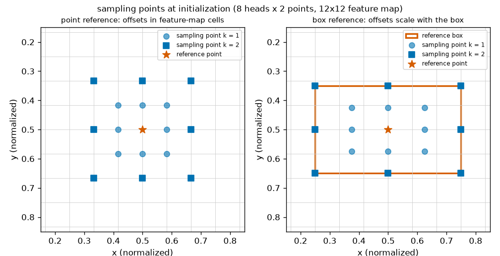
Let us check Figure 8-3 against the equations.
- Left (point reference). The \(k = 1\) sampling points are one cell, \(1/12 = 0.0833\), away from the reference point. With \(0.5 \pm 0.0833\), they land at \(0.4167\) and \(0.5833\). The \(k = 2\) points are two cells \(= 0.1667\) away, at \(0.3333\) and \(0.6667\). Together they evenly cover the 5×5-cell area around the reference point in eight directions.
- Right (box reference). The \(k = 1\) offset \((1, 1)\) becomes \(\big(\tfrac{1}{2} \cdot \tfrac{0.5}{2},\ \tfrac{1}{2} \cdot \tfrac{0.3}{2}\big) = (0.125,\ 0.075)\), so the sampling point is at \((0.625, 0.575)\). The \(k = 2\) offset \((2, 2)\) becomes \(\big(\tfrac{2}{2} \cdot 0.25,\ \tfrac{2}{2} \cdot 0.15\big) = (0.25,\ 0.15)\), so the sampling point is at \((0.75, 0.65)\), the bottom-right corner of the box. Sampling points with \(k = K\) lie on the box border, and the rest lie inside. The box is wide, so the pattern is wide too.
What this initialization does is "look evenly around the reference while nothing is known yet". As training proceeds, the offset layer's weights move away from 0, and the pattern becomes different for each query and each image. What it looks like after training is shown in Figure 8-9 at the end of this chapter.
Cost: number of positions read versus actual time
Let us count how cheap "looking only where it matters" is. First we count by hand, then we measure. To give it away up front: the two tell different stories.
Counting operations
The simplest yardstick is the number of (query, position) pairs read in one cross-attention. With \(N_q\) queries:
- Ordinary cross-attention: every cell per query → \(N_q \times HW\)
- Deformable attention: \(M \cdot L \cdot K\) sampling points per query → \(N_q \times MLK\)
With the same settings as the measurements later (100 queries, \(M = 8\), \(L = 1\), \(K = 2\)), growing the feature map gives the following. Deformable attention stays constant at \(100 \times 8 \times 1 \times 2 = 1{,}600\).
| Feature map | Cells \(HW\) | Ordinary: \(N_q \times HW\) | Deformable: \(N_q \times MLK\) | Ratio |
| 12×12 | 144 | 14,400 | 1,600 | 9× |
| 24×24 | 576 | 57,600 | 1,600 | 36× |
| 48×48 | 2,304 | 230,400 | 1,600 | 144× |
| 96×96 | 9,216 | 921,600 | 1,600 | 576× |
| 192×192 | 36,864 | 3,686,400 | 1,600 | 2,304× |
Let us also count at the size of a real model. RF-DETR Nano uses resolution 384 and patch size 16, so its feature map is 24×24 = 576 cells, with 300 queries and decoder cross-attention using 16 heads, 2 sampling points, and 1 level (the settings in the public code). Ordinary cross-attention would be \(300 \times 576 = 172{,}800\) pairs; deformable attention is \(300 \times 16 \times 1 \times 2 = 9{,}600\) pairs, one eighteenth as many.
But "number of positions read" is only part of the cost. Estimating the number of multiplications part by part gives a different picture. Small terms such as biases and softmax are left out.
- Estimated multiplications: 100 queries, D = 128, 12×12 map (HW = 144)
- \(\text{보통: 질의 · 출력 투영} = 2 \times N_q D^2 = 2 \times 100 \times 128^2 = 3{,}276{,}800\)
- (Ordinary: query and output projections.) Multiplying a length-\(D\) vector by a \(D \times D\) matrix takes \(D^2 = 16{,}384\) multiplications. For 100 queries, one query projection and one output projection.
- (Ordinary: key and value projections.) Key and value projections are applied to all 144 cells. This is independent of the number of queries and proportional to the number of cells.
- (Ordinary: scores and weighted sum.) One dot product per (query, cell) pair (\(D\) multiplications across all heads), and another \(D\) for the weighted sum of values. This is the 14,400 pairs counted in the table above times \(2D\).
- (Deformable: offset and weight prediction.) A linear layer producing \(2MLK + MLK = 3 \times 16 = 48\) numbers from each query's length-\(D\) vector. This is the \(O(3N_qCMK)\) term in Appendix A.1 of the paper.
- (Deformable: value projection; output projection.) Even in deformable attention, the value projection is applied to every cell (because the code projects first and reads afterward). With no keys, it is half that of ordinary attention.
- (Deformable: interpolation and weighted sum.) Reading one sampling point takes four neighbors × number of channels multiplications (each of the \(M\) heads reads \(D/M\) channels, so across heads it is \(4D\) for each of the \(LK\) sampling points), plus another \(D\) for the weighted sum. This is the \(5N_qKC\) term in A.1 of the paper, and the part that corresponds to the 1,600 pairs counted in the table.
- (Ordinary vs. deformable.) The totals. The number of pairs read differs by 9×, but the number of multiplications differs by only about 2.5×, because work present in both approaches, such as projections, makes up a large share.
Applying the same estimate to a 192×192 map (\(HW = 36{,}864\)), only the terms proportional to the number of cells grow, by 256×.
| Item (estimated multiplications) | 12×12 | 192×192 | With cell count |
| Ordinary: query and output projections | 3,276,800 | 3,276,800 | Constant |
| Ordinary: key and value projections | 4,718,592 | 1,207,959,552 | Proportional |
| Ordinary: scores and weighted sum | 3,686,400 | 943,718,400 | Proportional |
| Ordinary total | 11,681,792 | 2,154,954,752 | |
| Deformable: offset and weight prediction | 614,400 | 614,400 | Constant |
| Deformable: value projection | 2,359,296 | 603,979,776 | Proportional |
| Deformable: output projection | 1,638,400 | 1,638,400 | Constant |
| Deformable: interpolation and weighted sum | 128,000 | 128,000 | Constant |
| Deformable total | 4,740,096 | 606,360,576 |
At 192×192 the ratio between the two totals is about 3.6×, not "2,304×". What deformable attention makes independent of the cell count is the part where queries read values; applying the value projection to the whole feature map still remains. The paper captures this in its formulas too. It gives the complexity of ordinary attention as \(O(N_qC^2 + N_kC^2 + N_qN_kC)\) and that of deformable attention as \(O(2N_qC^2 + \min(HWC^2,\ N_qKC^2))\) (\(C\) is this chapter's \(D\), and \(N_k\) is the number of keys, \(HW\)). The first term of the \(\min\) is the cost of "project everything first", and the second is the cost of "project only the values read". With the second approach the cost becomes fully independent of the cell count. When the paper says the decoder's deformable cross-attention has "complexity \(O(NKC^2)\), independent of the spatial size \(HW\)", it refers to this second approach. The public code and this chapter's implementation use the first.
Measured times
We check whether the hand counts match actual time. nn.MultiheadAttention (ordinary cross-attention) and this chapter's MSDeformAttn get inputs of the same size, and the time of one forward pass is measured repeatedly (discarding the first 10 runs, then 50 runs) and the minimum is reported.
@torch.no_grad()
def complexity_table(device, sizes=(12, 24, 48, 96, 192), num_queries=100, dim=128, heads=8, points=2, batch=2,
                     repeats=50):
    """교차 어텐션 한 번의 "읽는 자리 수" 와 걸린 시간. 특징 맵 한 변을 키워 가며 잰다 (단일 레벨, L = 1)."""
    standard = nn.MultiheadAttention(dim, heads, batch_first=True).to(device).eval()
    deform = MSDeformAttn(dim, n_levels=1, n_heads=heads, n_points=points).to(device).eval()

    def clock(fn):
        times = []
        for _ in range(repeats + 10):
            start = time.perf_counter()
            fn()
            if device == "cuda":
                torch.cuda.synchronize()
            times.append(time.perf_counter() - start)
        return float(np.min(times[10:])) * 1000  # 처음 10번은 준비 운동으로 버리고 최솟값 (ms): 다른 일에 덜 흔들린다

    rows = []
    print(f"[계산량] 질의 {num_queries}개, 머리 M = {heads}, 레벨 L = 1, 표본점 K = {points}, D = {dim}, 배치 {batch}")
    print("특징 맵 | 토큰 HW | 보통: 질의×토큰 | 변형: 질의×M·L·K |  비   | 보통 ms | 변형 ms")
    for side in sizes:
        tokens = side * side
        memory = torch.randn(batch, tokens, dim, device=device)
        query = torch.randn(batch, num_queries, dim, device=device)
        reference = torch.rand(batch, num_queries, 1, 2, device=device)
        ms_standard = clock(lambda: standard(query, memory, memory, need_weights=False))
        ms_deform = clock(lambda: deform(query, reference, memory, [(side, side)]))
        pairs_standard, pairs_deform = num_queries * tokens, num_queries * heads * points
        rows.append((side, tokens, pairs_standard, pairs_deform, ms_standard, ms_deform))
        print(f"{side:3d}×{side:<3d} | {tokens:7d} | {pairs_standard:13,d} | {pairs_deform:14,d} | "
              f"{pairs_standard / pairs_deform:5.1f} | {ms_standard:7.2f} | {ms_deform:7.2f}")
    return rows
[계산량] 질의 100개, 머리 M = 8, 레벨 L = 1, 표본점 K = 2, D = 128, 배치 2
특징 맵 | 토큰 HW | 보통: 질의×토큰 | 변형: 질의×M·L·K |  비   | 보통 ms | 변형 ms
 12×12  |     144 |        14,400 |          1,600 |   9.0 |    2.69 |    7.06
 24×24  |     576 |        57,600 |          1,600 |  36.0 |    3.19 |    7.23
 48×48  |    2304 |       230,400 |          1,600 | 144.0 |    2.96 |    7.19
 96×96  |    9216 |       921,600 |          1,600 | 576.0 |    4.53 |    7.24
192×192 |   36864 |     3,686,400 |          1,600 | 2304.0 |   23.57 |    8.07
- Figure: Figure 8-4 Number of (query, position) pairs read in one cross-attention (left) and measured time (right). The horizontal axis is the feature map size; both axes are logarithmic. The solid orange line is ordinary cross-attention, the dashed blue line deformable attention.
- Left: as the feature map grows, the number of pairs read by ordinary cross-attention grows proportionally, while deformable attention stays constant at 1,600. Right: measured time. Deformable attention is nearly constant at 7 to 8 milliseconds, while ordinary attention is about 3 milliseconds on small maps and jumps to 24 milliseconds at 192×192, overtaking deformable attention.
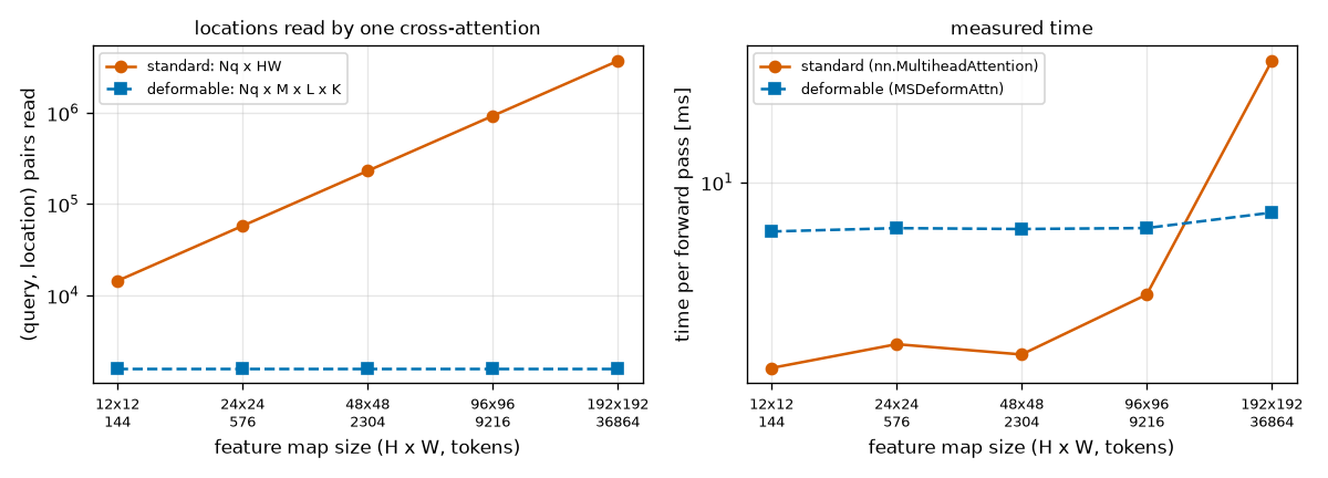
Three things can be read from Figure 8-4 and the table.
- Deformable attention's time is nearly independent of map size. While the cell count grew 256× (144 → 36,864), it only went from 7.06 ms to 8.07 ms. That it is not perfectly constant is probably because, as counted above, the value projection is proportional to the cell count.
- On small maps, deformable attention is actually slower. At 12×12, ordinary takes 2.69 ms and deformable 7.06 ms, so deformable attention is 2.6× slower, even though it needs fewer multiplications. In this tutorial's shapes world (12×12 maps), deformable attention gives no speed benefit.
- It reverses on large maps. Ordinary attention grows noticeably from 96×96 onward and reaches 23.57 ms at 192×192, 2.9× that of deformable attention (8.07 ms). In this measurement, the order flipped between 96×96 and 192×192.
This experiment did not separately measure why deformable attention is slow on small maps. A possible explanation is fixed overhead. In computations this small, "how many operations are launched" determines the time more than the number of multiplications. nn.MultiheadAttention finishes in a few well-optimized operations, whereas MSDeformAttn goes through four linear layers, a softmax, several reshapes, and an F.grid_sample per level. grid_sample is also an operation that reads scattered memory locations for each sampling point. The paper also notes that deformable attention pays the price of "unordered memory access" (Section 5.1).
- Caution: these times are for reference only
- These are minimum values measured on a laptop whose GPU was shared with other work. The direction, "deformable is slower on small maps and overtakes on large maps", was the same across several runs, but the crossover point and absolute values varied with run conditions. The numbers will differ on your device. The speed of a real model should be measured after exporting the whole model, as in Chapter 14.
So where does deformable attention's value lie? Table 1 of the paper offers a clue. Deformable DETR processes 19 images per second while using multi-scale features starting at stride 8, and DETR-DC5, which uses high-resolution features, processes 12. Meanwhile, the original DETR, which uses a single feature map, processes 28, faster than Deformable DETR. Deformable attention is not a component that makes things "faster on the same map" but one that "makes large maps and multiple maps affordable".
Multi-scale features
Why multiple resolutions?
Feature map resolution involves a trade-off. A fine map (small stride) captures the positions of small objects precisely, but each cell sees a narrow area and there are many cells. In a coarse map each cell summarizes a wide area and takes in large objects at a glance, but small objects get buried inside a single cell. Using several maps of different resolutions together is called multi-scale features.
Deformable DETR uses four levels (\(L = 4\)): three from applying 1×1 convolutions to the outputs of three ResNet backbone stages (strides 8, 16, 32), and one from applying a further 3×3 stride-2 convolution to the last stage's output (stride 64). All are set to 256 channels. In the paper's ablation (Table 2), switching from single-scale to multi-scale inputs raised AP by 1.7 and small-object AP by 2.9 (COCO, with \(K = 1\): 39.7 → 41.4, small objects 21.2 → 24.1).
Adding levels to deformable attention is cheap. The number of values a query reads only grows from \(MK\) to \(MLK\), and the reference point, being in normalized coordinates, is used as is at every level. With ordinary attention, the number of keys would grow by all the cells of the four levels concatenated (about 1.33× the finest level), and encoder self-attention would grow with the square of that.
Two levels in this chapter, one level in RF-DETR
This chapter's mini model uses two levels.
- Level 0 (12×12, stride 8): a 1×1 convolution on Chapter 7's backbone output.
- Level 1 (6×6, stride 16): a 3×3 stride-2 convolution on the same backbone output. This is the same way Deformable DETR builds its coarsest level.
Flattening each map into tokens and concatenating them gives \(144 + 36 = 180\) tokens. The tensor shape is (B, 180, D), and which tokens belong to which level is carried separately as spatial_shapes = [(12, 12), (6, 6)]. Deformable attention uses this list to turn the token sequence back into per-level maps (D, H_l, W_l) and then reads the sampling points.
- RF-DETR has one level
- In RF-DETR Nano, Small, and Medium, the projector passes only one feature map at stride 16 (
projector_scale=["P4"]in the public code) to the decoder, so \(L = 1\). Despite the name "multi-scale deformable attention", in practice 16 heads each read 2 sampling points at a single level (ca_nheads=16,dec_n_points=2). The structure in which the projector merges the outputs of several ViT backbone layers into one map is covered in Chapter 9 and Chapter 10. In this chapter's experiments too, reducing to one level made little difference (see the ablations later).
Refining boxes from a reference
In Chapter 7's DETR, the box head produced the four box numbers outright from the query vector alone: \(\hat{b} = \sigma(\operatorname{MLP}(\text{질의}))\) (질의 = query). With deformable attention, a query already has a reference point saying "around here". The features the query reads come from around that reference point, so it is more natural to produce the box as how far it deviates from the reference point. The paper explains that this eases optimization and ties the decoder's attention tightly to the predicted boxes, speeding up convergence (Section 4.1, Appendix A.3). The question is where to do the "add to the reference".
Inverse sigmoid
Normalized coordinates must lie between 0 and 1. Simply adding a head's change of \(0.2\) to a reference coordinate of \(0.95\) gives \(1.15\), outside the image. So the addition is done not in the 0 – 1 range but in logit space (all real numbers). The coordinate is converted back to a logit, the change is added there, and a sigmoid brings it back to 0 – 1. The function that converts a coordinate back to a logit is the inverse sigmoid \(\sigma^{-1}\).
\(\sigma^{-1}(x) = \log\frac{x}{1 - x}\)
This is exactly the formula obtained in Chapter 4 by solving the sigmoid \(p = 1/(1 + e^{-z})\) for \(z\): "the logit is the log-odds". There it turned a probability back into a logit; here it turns a coordinate back. Let us confirm once that it really is the inverse.
- Check: feeding the inverse sigmoid into the sigmoid returns the input
- \(\sigma\big(\sigma^{-1}(x)\big) = \frac{1}{1 + e^{-\log\frac{x}{1 - x}}}\)
- Substituted \(\log\frac{x}{1-x}\) for \(z\) in the sigmoid definition \(\sigma(z) = 1/(1 + e^{-z})\).
- Since \(e^{-\log a} = 1/a\), \(e^{-\log\frac{x}{1-x}} = \frac{1-x}{x}\).
- Putting the denominator over a common denominator brings us back to \(x\). With numbers: \(\sigma^{-1}(0.3) = \log\frac{0.3}{0.7} = \log 0.4286 = -0.8473\) and \(\sigma(-0.8473) = 0.3\).
A few values in a table. The middle value \(0.5\) has logit 0, and the logit grows without bound as the coordinate approaches 0 or 1.
| Coordinate \(x\) | 0.05 | 0.1 | 0.25 | 0.3 | 0.5 | 0.95 |
| \(\sigma^{-1}(x)\) | \(-2.9444\) | \(-2.1972\) | \(-1.0986\) | \(-0.8473\) | \(0\) | \(2.9444\) |
def inverse_sigmoid(x: torch.Tensor, eps: float = 1e-5) -> torch.Tensor:
    """시그모이드의 역함수 σ⁻¹(x) = log(x / (1 − x)). 0 – 1 의 좌표를 "로짓 공간" 으로 되돌린다.

    x 가 0 이나 1 에 닿으면 값이 ±∞ 가 되므로 분자 · 분모를 eps 이상으로 자른다.
    """
    x = x.clamp(min=0.0, max=1.0)
    return torch.log(x.clamp(min=eps) / (1 - x).clamp(min=eps))
If \(x\) is exactly 0 or 1, \(\log 0\) or division by zero would occur, so the code clips the numerator and denominator to at least \(10^{-5}\). The logit then stays within about \(\pm 11.5\).
Adding in logit space
With the reference box \(b^{\text{ref}}\) and the four numbers produced by the box head \(\Delta b\) ("delta b"), the new box is as follows. It is applied separately to each of the box's four components \((c_x, c_y, w, h)\).
\(\hat{b} = \sigma\big(\Delta b + \sigma^{-1}(b^{\text{ref}})\big)\)
- What this equation does
- \(\Delta b = 0 \quad\Longrightarrow\quad \hat{b} = \sigma\big(\sigma^{-1}(b^{\text{ref}})\big) = b^{\text{ref}}\)
- If the head outputs 0, the box stays at the reference. So if the box head's last layer is initialized to 0, every predicted box equals its reference box at the start of training.
- (For every real \(z\).) The sigmoid's value is always between 0 and 1. However large or small \(\Delta b\) is, \(\hat{b}\) never leaves the image. No separate clipping is needed.
- The property from Chapter 4, \(\sigma'(z) = \sigma(z)(1 - \sigma(z))\). It is the rate at which the coordinate changes when \(\Delta b\) changes slightly. It is largest, \(0.25\), in the middle (\(\hat{b} = 0.5\)), and shrinks toward the edges.
- Comparing the logits of both sides gives \(\log\frac{\hat{b}}{1 - \hat{b}} = \Delta b + \log\frac{b^{\text{ref}}}{1 - b^{\text{ref}}}\); this is its exponential. Adding \(\Delta b\) to the logit multiplies the odds \(\frac{b}{1-b}\) by \(e^{\Delta b}\). This suits values like width and height, where "how many times larger" is the natural question.
Let us plug in numbers.
- By hand: reference 0.30 with Δ = 0.5
- \(\sigma^{-1}(0.30) = \log\frac{0.30}{0.70} = -0.8473\)
- Converted the reference coordinate back to a logit.
- Added the head's output \(\Delta b = 0.5\) in logit space.
- Back to 0 – 1 through the sigmoid. The coordinate moved \(0.114\), from \(0.30\) to \(0.414\). Plugging the reference value into the approximation \(\hat{b}(1 - \hat{b})\,\Delta b\) gives \(0.3 \times 0.7 \times 0.5 = 0.105\), which is close.
| Reference \(b^{\text{ref}}\) | \(\Delta b\) | \(\sigma^{-1}(b^{\text{ref}})\) | Summed logit | New value \(\hat{b}\) | With plain addition |
| 0.30 | \(+0.5\) | \(-0.8473\) | \(-0.3473\) | 0.4140 | 0.80 |
| 0.50 | \(+0.5\) | \(0\) | \(0.5\) | 0.6225 | 1.00 |
| 0.95 | \(+2.0\) | \(2.9444\) | \(4.9444\) | 0.9929 | 2.95 (outside the image) |
| 0.10 | \(-1.0\) | \(-2.1972\) | \(-3.1972\) | 0.0393 | \(-0.90\) (outside the image) |
| 0.20 | \(+1.0\) | \(-1.3863\) | \(-0.3863\) | 0.4046 | 1.20 (outside the image) |
Read the last row as a width. The odds of a reference width of \(0.20\) are \(0.2/0.8 = 0.25\), and \(\Delta b = 1\) multiplies them by \(e^{1} = 2.718\) to give \(0.6796\). Converting odds of \(0.6796\) back to a value gives \(0.6796/1.6796 = 0.4046\). The width roughly doubled. Near the edges, as in the third row, the same \(\Delta b\) moves the coordinate only a little. Addition in logit space automatically becomes more cautious near 0 and 1.
Repeating layer by layer: iterative box refinement
The decoder has several layers. In Chapter 7 each layer produced its box from scratch, but now the box produced by the previous layer can serve as the next layer's reference. Writing the box produced by the \(d\)-th decoder layer as \(\hat{b}^{d}\) (the superscript is a layer index, not a power):
\(\hat{b}^{d} = \sigma\Big(\Delta b^{d} + \sigma^{-1}\big(\operatorname{sg}(\hat{b}^{d-1})\big)\Big), \qquad d = 1, 2, \dots\)
This is iterative bounding box refinement. \(\Delta b^{d}\) is the change produced by the \(d\)-th layer's box head, and \(\operatorname{sg}(\cdot)\) is stop-gradient: the value in parentheses is used as is, but during backpropagation it is treated as a constant and no gradient flows through it. Instead of one layer getting the box right in one shot, each layer corrects the previous layer's answer a little. The paper says it took this idea from iterative refinement in optical flow estimation (Teed & Deng, 2020). Four further conventions come with it.
- Each layer has its own box head (weights are not shared), because the layers do different jobs: the first moves boxes a lot, later ones fine-tune. In Chapter 7's DETR, all layers shared one head.
- Deformable attention's reference changes too. The \(d\)-th layer's cross-attention uses \(\hat{b}^{d-1}\) as its reference box, starting from the center \((c_x, c_y)\) and multiplying the offsets by \((w, h)\) (the "box reference" equation earlier). As the box gets closer to the object, the sampling points also gather on the object.
- The gradient is cut when passing to the next layer. \(\operatorname{sg}(\hat{b}^{d-1})\) means the value is used as is but treated as a constant during backpropagation (
box.detach()in the code). - The first layer's reference is a point. At first there is no box, only the reference point \(p_q\), so the first layer starts only the center from the reference point, and the head produces width and height outright (the equation in Appendix A.3 of the paper). \(\hat{b}^{1} = \Big(\sigma\big(\Delta b_x + \sigma^{-1}(p_x)\big),\ \ \sigma\big(\Delta b_y + \sigma^{-1}(p_y)\big),\ \ \sigma(\Delta b_w),\ \ \sigma(\Delta b_h)\Big)\)
- Differences between the paper's appendix and the public code
- Appendix A.4 of the paper gives the initial box for iterative refinement as \(\hat{b}^{0} = (p_x,\ p_y,\ 0.1,\ 0.1)\), i.e., the reference point with width and height 0.1 attached (it reports similar results with other values between 0.05 and 0.5). The behavior of the public implementation, as checked while preparing this chapter, is slightly different. The first layer uses a 2D reference point, the head directly produces width and height as in item 4 above, and that head's width/height bias is initialized to \(-2.0\) (\(\sigma(-2) = 0.1192\), so the initial box size is about 0.12). This chapter's implementation follows the latter. So layer 1 uses "reference = point" and layers 2 and 3 use "reference = box". However, the official Deformable DETR repository could not be opened directly in this environment; this was confirmed using the RF-DETR source, which inherited the same code.
Why cut the gradient
What happens if the gradient is not cut? Layer 3's box \(\hat{b}^{3}\) depends on \(\hat{b}^{1}\) through \(\hat{b}^{2}\), so layer 3's box loss flows back to the box heads of layers 1 and 2. Layer 1's head then receives both a signal to fit its own box to the ground truth (layer 1's auxiliary loss) and a signal to "produce a box that makes it easy for layer 3 to get it right". Since deformable attention's sampling locations also depend on the reference box, gradients get tangled along that path too. The paper states that, to stabilize training, gradients flow only through \(\Delta b^{d}\) and are blocked at \(\sigma^{-1}(\hat{b}^{d-1})\).
Once cut, the roles are clean. Each layer's box head learns only "how much to correct the given reference". The reference itself is the previous layer's responsibility, through its own loss. Only the box-coordinate path is cut. The query vector passes from layer to layer uncut, so later layers' losses still train earlier layers' attention and FFN through the query vector.
- In RF-DETR
- The framework "box = reference + change produced by the head" carries all the way to RF-DETR. Two things change, though. The addition is not in logit space but a box reparameterization (of the form \(c_x = \delta_x w + x\), \(w' = e^{\delta_w} w\), Chapter 9), and the public code's default setting (
lite_refpoint_refine=True) does not swap the reference box at each layer; instead all decoder layers share the initial reference box (Chapter 10). This chapter's layer-by-layer refinement is the method of its prototype, Deformable DETR.
Sigmoid-based classification and matching
Deformable DETR also changes classification. It is a single line in the paper's implementation details: classification uses focal loss (loss weight 2), and the number of object queries goes from 100 to 300. This change is part of the line that continues to RF-DETR (LW-DETR and RF-DETR go one step further and use an IoU-aware BCE loss; see Chapter 9).
Without a ∅ class
Chapter 7's DETR classified with a 4-way softmax: 3 classes plus "no object" ∅. In the terms of Chapter 4, this is the "background class" approach. Deformable DETR uses a separate sigmoid per class. The classification head produces 3 logits per query, each answering a yes/no question: "Is this query a circle?", "A rectangle?", "A triangle?"
- The target is a 0/1 matrix of shape
(B, N, 클래스 수)(number of classes). For queries paired with a ground truth by Hungarian matching, only the ground-truth class entry is 1; everything else is 0. - Unpaired queries have all three entries at 0. "No object" is not given its own entry but expressed as "none of the classes".
- Chapter 4's focal loss \(\mathrm{FL} = -\alpha_t (1 - p_t)^{\gamma} \log p_t\) (\(\alpha = 0.25\), \(\gamma = 2\)) is computed for each entry, summed, and divided by the number of ground-truth objects in the batch. The loss coefficient is 2.
- The classification head's bias is \(-\log 99 = -4.5951\), following Chapter 4's prior-probability bias initialization. At first every entry answers "about 1%".
Counting for this chapter's model, one image has 12 queries × 3 classes = 36 entries, of which only 1 – 4 (the number of objects) are positive. On COCO, with 300 queries and dozens of classes, the entries number well over ten thousand while positives are only as many as the objects in the image. This is exactly the "overwhelmingly negative" situation seen in Chapter 4, which focal loss targets. Compare this with how Chapter 7's DETR handled the same imbalance by lowering the ∅ class weight to 0.1.
Right at the start of training, the loss of one positive entry at \(p = 0.01\) is \(0.25 \times 0.99^2 \times (-\log 0.01) = 0.25 \times 0.9801 \times 4.6052 = 1.1284\), and that of one negative entry is \(0.75 \times 0.01^2 \times (-\log 0.99) = 0.75 \times 0.0001 \times 0.01005 = 7.5 \times 10^{-7}\). Just as computed in Chapter 4, nearly all of the loss comes from positive entries.
Post-processing at inference changes too. With no ∅, instead of "the maximum excluding ∅", the sigmoid probabilities of the \(12 \times 3 = 36\) (query, class) pairs are flattened into one list and the 12 highest-scoring ones are output as predictions. Because selection is per pair, one query may be selected twice under two classes.
A focal-style matching cost
When the loss changes, the matching cost changes to match. Chapter 7's classification cost was \(-\hat{p}_i(c_j)\), the negative of the softmax probability given to the ground-truth class. Now, writing \(\hat{p}\) for short for the sigmoid probability that prediction \(i\) gives to the entry of ground truth \(j\)'s class \(c_j\), the classification cost is as follows.
\(C_{\text{cls}}(i, j) = \underbrace{\alpha\,(1 - \hat{p})^{\gamma}\,(-\log \hat{p})}_{\text{양성으로 볼 때의 손실}} \;-\; \underbrace{(1 - \alpha)\,\hat{p}^{\,\gamma}\,\big(-\log(1 - \hat{p})\big)}_{\text{음성으로 볼 때의 손실}}, \qquad \alpha = 0.25,\ \gamma = 2\)
Both terms are Chapter 4's focal loss. The first term (labeled "loss if treated as positive") is its value when the entry's target is 1 (\(p_t = \hat{p}\), \(\alpha_t = \alpha\)), and the second (labeled "loss if treated as negative") is its value when the target is 0 (\(p_t = 1 - \hat{p}\), \(\alpha_t = 1 - \alpha\)). Following the loss shows why one is subtracted from the other.
- Classification cost = change in loss from pairing
- \(\text{예측 } i \text{ 를 정답 } j \text{ 와 짝지으면}: \quad \text{칸 } (i, c_j) \text{ 의 목표} = 1, \quad \text{손실} = \alpha\,(1 - \hat{p})^{\gamma}\,(-\log \hat{p})\)
- (If prediction \(i\) is paired with ground truth \(j\): the target of entry \((i, c_j)\) is 1.) The ground-truth class entry of a paired query becomes positive. This is that entry's focal loss.
- (If not paired: the target of entry \((i, c_j)\) is 0.) Without a pair, the same entry remains negative. This is the focal loss in that case.
- (The entry's loss if paired minus the entry's loss if not paired.) The difference between the two cases. The cost is how much the entry's classification loss increases (or decreases, if negative) by choosing this pair. Since Hungarian matching picks the assignment with the smallest total cost, it favors pairs that reduce the classification loss the most.
Let us compute the values for various probabilities \(\hat{p}\). For example, with \(\hat{p} = 0.9\):
- By hand: classification cost at predicted probability 0.9
- \(\alpha\,(1 - \hat{p})^{\gamma}\,(-\log \hat{p}) = 0.25 \times 0.1^2 \times 0.10536 = 0.00026\)
- Loss if treated as positive. It is already right at 0.9, so this is tiny. \(-\log 0.9 = 0.10536\).
- Loss if treated as negative. It gave 0.9 to an entry that should be 0, so this is large. \(-\log 0.1 = 2.30259\).
- Pairing this prediction with this ground truth reduces the entry's loss by about 1.4. The cost is strongly negative, so matching welcomes this pair.
| Predicted probability \(\hat{p}\) | 0.01 | 0.1 | 0.3 | 0.5 | 0.7 | 0.9 | 0.99 |
| Loss if treated as positive | 1.1284 | 0.4663 | 0.1475 | 0.0433 | 0.0080 | 0.0003 | 0.0000 |
| Loss if treated as negative | 0.0000 | 0.0008 | 0.0241 | 0.1300 | 0.4425 | 1.3988 | 3.3851 |
| Focal classification cost \(C_{\text{cls}}\) | \(+1.1284\) | \(+0.4655\) | \(+0.1234\) | \(-0.0866\) | \(-0.4344\) | \(-1.3986\) | \(-3.3851\) |
| Chapter 7 DETR classification cost \(-\hat{p}\) | \(-0.01\) | \(-0.1\) | \(-0.3\) | \(-0.5\) | \(-0.7\) | \(-0.9\) | \(-0.99\) |
Both costs decrease as the probability rises, favoring predictions that rate the ground-truth class highly. The difference is the range. Chapter 7's \(-\hat{p}\) is confined between \(-1\) and 0, while the focal cost drops without bound as the probability approaches 1. Also, at the start (\(\hat{p} = 0.01\)) it is positive, \(+1.13\). However, matching always assigns one prediction to each ground truth, so what decides the assignment is the differences between predictions rather than the sign of the cost.
The full matching cost is Chapter 7's formula with only the class term replaced: \(C_{ij} = 2\,C_{\text{cls}}(i, j) + 5\,\lVert \hat{b}_i - b_j \rVert_1 - 2\,\operatorname{GIoU}(\hat{b}_i, b_j)\). In Chapter 7 the classification coefficient was 1; the two box terms (L1 distance and GIoU, Chapter 2) and their coefficients are unchanged. RF-DETR's public code uses this formula and these coefficients as well. Passing class_cost="focal" to Chapter 7's HungarianMatcher gives this cost.
What changed from Chapter 7
The table below collects how this chapter's mini model MiniDeformableDETR differs from Chapter 7's MiniDETR. Keep this table in mind when reading the results later. More than one thing changed.
| Item | Chapter 7 MiniDETR | Chapter 8 MiniDeformableDETR (main model) |
| Backbone | 6 convolutional layers, 12×12 map | Same |
| Encoder | 3 layers of global self-attention | None (backbone features go straight to the decoder) |
| Features read by the decoder | One 12×12 map (144 tokens) | Two levels, 12×12 and 6×6 (180 tokens) |
| Cross-attention | All 144 cells, query–key dot product | Deformable attention: 8 · 2 · 2 = 32 sampling points |
| Query position | Learned position embedding only | Position embedding + a reference point derived from it |
| Box prediction | The head outputs all four numbers outright | Change from the reference (in logit space), refined layer by layer |
| Box and classification heads | One shared by all layers | Separate per layer |
| Classification | 4-way softmax (including ∅) | 3 per-class sigmoids |
| Classification loss | Cross-entropy (∅ weight 0.1), coefficient 1 | Focal loss (\(\alpha\) 0.25, \(\gamma\) 2), coefficient 2 |
| Classification head bias | Ordinary initialization | \(-4.5951\) (prior probability 0.01) |
| Matching cost | \(-\hat{p}_i(c_j) + 5\,\lVert \hat{b}_i - b_j \rVert_1 - 2\,\operatorname{GIoU}\) | \(2\,C_{\text{cls}} + 5\,\lVert \hat{b}_i - b_j \rVert_1 - 2\,\operatorname{GIoU}\) (\(C_{\text{cls}}\) in focal form) |
| Post-processing | Per-query maximum excluding ∅ | Top 12 of the 36 (query, class) pairs |
| Learning rate | 2e-4 for everything | 2e-4, except 2e-5 for the linear layers producing offsets and reference points |
| Number of parameters | 1,333,608 | 1,091,607 |
| Kept the same | Data (4,000 training and 500 validation images), 12 queries, \(D = 128\), 8 heads, 3 decoder layers, FFN 256, AdamW, batch 32, 60 epochs (learning rate ×1/10 after epoch 48), gradient clipping 0.1, seed 0, auxiliary losses | |
Two-stage query selection
Choosing references by looking at the image
So far, the reference points have been independent of the image. Each query has a learned embedding, and a linear layer plus sigmoid applied to it gives the reference point. Whatever image comes in, the 12 reference points are in the same places. If an object is far from a reference point, the first decoder layer has to move it a long way.
The two-stage scheme chooses references by looking at the image. In the paper's words, it is a variant inspired by two-stage detectors. In the first stage, every cell of the feature map acts as an object query and produces a region proposal, "if there is an object here, this is its box", together with a score; the few highest-scoring ones are passed to the second stage (the decoder) as its initial reference boxes. The paper notes that NMS is not applied to the proposals selected in the first stage.
Here, step by step, is what this chapter's implementation (two_stage=True) does. The feature tokens number 180: 144 from level 0 and 36 from level 1.
- Place one fixed starting box per cell: at the cell center, with a size set by the level.
- Apply a linear layer and layer normalization to the cell's feature vector, then produce 3 class logits with a classification head and 4 deltas with a box head (a 3-layer MLP). The tensor shapes are
(B, 180, 3)and(B, 180, 4). - Add the deltas to the starting boxes in logit space to get a proposal box per cell. This is the same formula as iterative box refinement.
- Take the maximum of each cell's 3 class logits as that cell's score, and pick the top \(N = 12\) cells by score.
- Use the 12 selected proposal boxes, with gradients cut, as the decoder's initial reference boxes. From the first decoder layer on, "reference = box".
- Apply the same loss as for the decoder layers' outputs (Hungarian matching + focal, L1, GIoU) to the 12 selected logits and boxes as well. This loss trains the heads of steps 2 – 4.
The proposal box grid and deltas
The starting box from step 1, at cell (row \(r\), column \(c\)) of level \(l\), is as follows. \(s = 0.05\) is the base size.
\(b^{\text{격자}}_{l,r,c} = \Big(\frac{c + 0.5}{W_l},\ \ \frac{r + 0.5}{H_l},\ \ s \cdot 2^{l},\ \ s \cdot 2^{l}\Big), \qquad \hat{b}^{\text{제안}} = \sigma\Big(\Delta b + \sigma^{-1}\big(b^{\text{격자}}\big)\Big)\)
(Superscripts: 격자 = grid, 제안 = proposal.) The center is the cell center (the same coordinate convention used for bilinear interpolation), and the width and height are \(0.05\) at level 0 and \(0.1\) at level 1. Cells on coarser levels start from larger boxes. The equation in Appendix A.4 of the paper is the same (it counts levels from 1 and writes \(2^{l-1}s\), with \(s = 0.05\)).
def gen_proposals(spatial_shapes, base_scale: float = 0.05, device=None) -> torch.Tensor:
    """2단계의 1단계: 특징 맵의 칸마다 "제안 박스" 하나를 놓는다. 돌려주는 값: (ΣHW, 4) 정규화 (cx, cy, w, h).

    중심은 칸의 중심 ((c + 0.5)/W, (r + 0.5)/H), 너비 · 높이는 레벨 l 에서 base_scale · 2^l 로 고정
    (RF-DETR 공식 구현의 gen_encoder_output_proposals 와 같다. 해상도가 낮은 레벨일수록 큰 박스를 맡는다).
    토큰 순서(레벨 0 의 행 우선, 이어서 레벨 1 …)는 memory 와 같다. 모델은 이 박스에 델타를 더해 고친다.
    """
    proposals = []
    for level, (height, width) in enumerate(spatial_shapes):
        ys = (torch.arange(height, dtype=torch.float32, device=device) + 0.5) / height
        xs = (torch.arange(width, dtype=torch.float32, device=device) + 0.5) / width
        grid_y, grid_x = torch.meshgrid(ys, xs, indexing="ij")
        size = torch.full_like(grid_x, base_scale * 2.0**level)
        proposals.append(torch.stack([grid_x, grid_y, size, size], dim=-1).reshape(-1, 4))
    return torch.cat(proposals)
gen_proposals([(12, 12), (6, 6)]): (180, 4), 첫 칸 [0.0417 0.0417 0.05 0.05 ], 레벨 1 의 첫 칸 [0.0833 0.0833 0.1 0.1 ]
The center of the first cell (level 0, row 0, column 0) is \(0.5/12 = 0.0417\), and that of level 1's first cell is \(0.5/6 = 0.0833\). Let us compute, for one cell, how large the delta must be for a starting box to become an actual object's box.
- By hand: from a starting box to a box of width 0.25
- \(b^{\text{격자}}_{0,5,7} = \Big(\frac{7.5}{12},\ \frac{5.5}{12},\ 0.05,\ 0.05\Big) = (0.6250,\ 0.4583,\ 0.05,\ 0.05)\)
- The starting box of cell (row 5, column 7) on level 0. Its size is \(0.05 \times 2^0 = 0.05\), or 4.8 pixels in a 96-pixel image, much smaller than the shapes in the shapes world (side 0.14 – 0.42).
- Solve for the delta needed for the width to become 0.25. Took the inverse sigmoid of both sides and moved \(\sigma^{-1}(0.05)\) across.
- From the earlier table, \(\sigma^{-1}(0.25) = -1.0986\) and \(\sigma^{-1}(0.05) = -2.9444\). In terms of odds, this scales \(0.05/0.95 = 0.0526\) up to \(0.25/0.75 = 0.3333\), i.e., by \(e^{1.8458} = 6.33\) times.
- (Starting from a level-1 cell.) If a level-1 cell (starting width 0.1) takes the same object, the required delta is smaller. Starting sizes differ by level so that coarse levels can easily take large objects and fine levels small ones.
The code for steps 2 – 5 is shown with the model in "Reading the implementation" below (select_queries). A note on the rest of the query: the content of the queries entering the decoder is still the learned embedding query_feat, not the selected cells' features, and the queries' position embedding is made by feeding the sine embedding (Chapter 5) of the selected reference box's four numbers into a 2-layer MLP. The LW-DETR paper calls this scheme, with position from the image and content from learned values, "mixed query selection".
Differences from the original Deformable DETR
This chapter's two-stage implementation does not follow the Deformable DETR paper exactly; it follows what RF-DETR's public code does, so that it can be carried straight into Chapter 10. The differences are listed here.
| Item | Deformable DETR paper (Appendix A.4) | This chapter's implementation (RF-DETR style) |
| First-stage classification | Binary foreground/background classification | Produces per-class logits (3) and selects by their maximum |
| First-stage loss | DETR's Hungarian loss on every cell's prediction | Hungarian loss on the \(N\) selected only |
| Position embedding of decoder queries | Position embedding of the proposal coordinates | Same (sine embedding of the reference box → MLP) |
| Content of decoder queries | Not stated in the paper's main text. The public implementation is understood to derive it from the embedding of the proposal coordinates as well, but this could not be checked directly in this environment | Learned embedding |
| Starting box | Cell coordinates, size \(2^{l-1}s\), \(s = 0.05\) | Same |
| Encoder before the decoder | Proposals from the output of a deformable self-attention encoder | Proposals from backbone features with no encoder (in RF-DETR, the output of the ViT + projector) |
Some differences from RF-DETR also remain. RF-DETR handles proposals and reference boxes with box reparameterization, adds a learned refpoint_embed to the selected boxes, uses 13 query groups during training (Group DETR), and does not swap reference boxes at each layer. These are not included in this chapter; they are added one at a time in Chapter 9 and Chapter 10. Two-stage query selection itself is revisited in detail in Chapter 10 alongside RF-DETR's actual code.
Reading the implementation
code/ch08_deformable.py reuses the backbone (SmallBackbone), Hungarian matching (HungarianMatcher), set loss (SetCriterion), and training loop (fit) from Chapter 7's ch07_detr.py, and builds only what is new in this chapter. We skip inverse_sigmoid, bilinear_sample, and gen_proposals, already seen, and read the rest.
The deformable attention module
First, the part inside the brackets of the equation: "read at the sampling points and take a weighted sum". The inputs are the values, already value-projected and split per head, (B, M, C/M, ΣHW); the sampling point coordinates (B, Nq, M, L, K, 2); and the weights (B, Nq, M, L, K) (here C is \(D\) in the text, and ΣHW is the total number of cells across all levels).
def ms_deform_attn_core(value, spatial_shapes, sampling_locations, attention_weights):
    """변형 어텐션의 핵심: 표본점에서 값을 읽어(쌍선형 보간) 어텐션 가중치로 가중합한다.

    value               (B, M, C/M, ΣHW)      머리별로 나눈 값 (모든 레벨을 이어 붙인 토큰)
    spatial_shapes      [(H_0, W_0), …]       레벨마다의 특징 맵 크기
    sampling_locations  (B, Nq, M, L, K, 2)   표본점의 정규화 좌표 (x, y)
    attention_weights   (B, Nq, M, L, K)      머리마다 L·K 개 표본점에 걸친 합이 1
    돌려주는 값          (B, Nq, C)            머리 M 개의 결과를 이어 붙인 것
    """
    batch, heads, head_dim, _ = value.shape
    num_queries = sampling_locations.shape[1]
    levels = value.split([h * w for h, w in spatial_shapes], dim=-1)
    grids = 2 * sampling_locations - 1  # grid_sample 은 좌표를 −1 – 1 로 받는다
    sampled = []
    for level, (height, width) in enumerate(spatial_shapes):
        value_map = levels[level].reshape(batch * heads, head_dim, height, width)  # 머리를 배치 축으로
        grid = grids[:, :, :, level].transpose(1, 2).flatten(0, 1)  # (B·M, Nq, K, 2)
        # (B·M, C/M, Nq, K): 질의 Nq 개 × 표본점 K 개 자리의 값. bilinear_sample 과 같은 계산을 한꺼번에 한다
        sampled.append(F.grid_sample(value_map, grid, mode="bilinear", padding_mode="zeros", align_corners=False))
    sampled = torch.stack(sampled, dim=-2).flatten(-2)  # (B·M, C/M, Nq, L·K)
    weights = attention_weights.transpose(1, 2).reshape(batch * heads, 1, num_queries, -1)  # (B·M, 1, Nq, L·K)
    output = (sampled * weights).sum(-1)  # (B·M, C/M, Nq): 표본점에 걸친 가중합
    return output.view(batch, heads * head_dim, num_queries).transpose(1, 2)  # (B, Nq, C)
The shape changes several times, so let us follow it line by line.
-
value.split(...): cuts the concatenated tokens by level. Level 0 is(B, M, C/M, 144)and level 1 is(B, M, C/M, 36). -
reshape(batch * heads, head_dim, height, width): merges heads into the batch axis to form an "image" of shape(B·M, C/M, H, W). This is because each head reads a different channel group at different sampling points. -
grids = 2 * sampling_locations - 1: converts normalized coordinates togrid_sample's \(-1\) – \(1\) coordinates. The grid for one level is(B·M, Nq, K, 2). -
F.grid_sample(...):(B·M, C/M, Nq, K), the values read by bilinear interpolation atNqqueries ×Ksampling points. It does the same computation asbilinear_sampleabove, all at once. -
torch.stack(..., dim=-2).flatten(-2): combines the levels into(B·M, C/M, Nq, L·K). - Multiplying by the weights
(B·M, 1, Nq, L·K)and summing over the last axis gives(B·M, C/M, Nq), which is turned back into(B, Nq, C). The results of the \(M\) heads end up concatenated along the channel axis.
The module wrapping this function is MSDeformAttn. It contains the four linear layers, their initialization, and the branch for point versus box references.
class MSDeformAttn(nn.Module):
    """다중 스케일 변형 어텐션 (Deformable DETR). 매개변수 이름 · 초기화는 공식 구현과 같다.

    질의 하나가 하는 일 (머리 m = 1 … M, 레벨 l = 1 … L, 표본점 k = 1 … K):
      1) 오프셋 Δp_mlk = Linear(질의)            — 기준점에서 얼마나 떨어진 곳을 볼지 (2차원)
      2) 가중치 A_mlk  = softmax(Linear(질의))   — 머리마다 L·K 개에 걸쳐 합이 1
      3) 값     x(p + Δp_mlk)                    — 값 투영을 거친 특징 맵에서 쌍선형 보간으로 읽는다
      4) 출력   = 출력 투영( 머리마다 Σ_l Σ_k A_mlk · x_l(p_l + Δp_mlk) 를 이어 붙인 것 )
    열쇠와의 내적이 없다: "어디를 볼지" 도 "얼마나 볼지" 도 질의만 보고 정한다.
    """

    def __init__(self, d_model: int = 128, n_levels: int = 2, n_heads: int = 8, n_points: int = 2):
        super().__init__()
        assert d_model % n_heads == 0
        self.d_model, self.n_levels, self.n_heads, self.n_points = d_model, n_levels, n_heads, n_points
        self.sampling_offsets = nn.Linear(d_model, n_heads * n_levels * n_points * 2)
        self.attention_weights = nn.Linear(d_model, n_heads * n_levels * n_points)
        self.value_proj = nn.Linear(d_model, d_model)
        self.output_proj = nn.Linear(d_model, d_model)
        self._reset_parameters()

    def _reset_parameters(self):
        # 오프셋: 가중치는 0, 편향만 정해 준다 → 처음에는 어떤 질의든 같은 무늬로 표본점을 찍는다.
        # 머리 m 은 각도 2πm/M 방향을 맡고(최댓값 노름으로 나눠 정사각형 테두리 위의 8방향이 된다),
        # k 번째 표본점은 그 방향으로 k 칸 떨어진 곳 → 기준점 주위를 골고루 본다.
        nn.init.constant_(self.sampling_offsets.weight, 0.0)
        thetas = torch.arange(self.n_heads, dtype=torch.float32) * (2.0 * math.pi / self.n_heads)
        grid = torch.stack([thetas.cos(), thetas.sin()], -1)  # (M, 2)
        grid = grid / grid.abs().max(-1, keepdim=True)[0]
        grid = grid.view(self.n_heads, 1, 1, 2).repeat(1, self.n_levels, self.n_points, 1)  # (M, L, K, 2)
        for k in range(self.n_points):
            grid[:, :, k, :] *= k + 1
        with torch.no_grad():
            self.sampling_offsets.bias = nn.Parameter(grid.view(-1))
        # 어텐션 가중치: 가중치 · 편향 모두 0 → 소프트맥스를 거치면 모든 표본점이 1/(L·K) 로 같다
        nn.init.constant_(self.attention_weights.weight, 0.0)
        nn.init.constant_(self.attention_weights.bias, 0.0)
        nn.init.xavier_uniform_(self.value_proj.weight)
        nn.init.constant_(self.value_proj.bias, 0.0)
        nn.init.xavier_uniform_(self.output_proj.weight)
        nn.init.constant_(self.output_proj.bias, 0.0)

    def forward(self, query, reference_points, value, spatial_shapes, return_details: bool = False):
        """query            (B, Nq, C)
        reference_points (B, Nq, L, 2) 기준점 (x, y)  또는  (B, Nq, L, 4) 기준 박스 (cx, cy, w, h) — 정규화 0 – 1
        value            (B, ΣHW, C)  레벨 0 의 토큰 H_0·W_0 개, 레벨 1 의 토큰 … 을 차례로 이어 붙인 것 (행 우선)
        spatial_shapes   [(H_0, W_0), …, (H_{L−1}, W_{L−1})]
        돌려주는 값: (B, Nq, C).  return_details=True 면 (출력, 표본점 (B, Nq, M, L, K, 2), 가중치 (B, Nq, M, L, K)).
        """
        batch, num_queries, _ = query.shape
        heads, levels, points = self.n_heads, self.n_levels, self.n_points
        assert value.shape[1] == sum(h * w for h, w in spatial_shapes)

        value = self.value_proj(value)  # (B, ΣHW, C)
        value = value.transpose(1, 2).reshape(batch, heads, self.d_model // heads, -1)  # (B, M, C/M, ΣHW)
        offsets = self.sampling_offsets(query).view(batch, num_queries, heads, levels, points, 2)
        weights = self.attention_weights(query).view(batch, num_queries, heads, levels * points)
        weights = weights.softmax(-1).view(batch, num_queries, heads, levels, points)

        if reference_points.shape[-1] == 2:
            # 기준이 점: 오프셋의 단위는 "그 레벨 특징 맵의 칸". (W_l, H_l) 로 나눠 정규화 좌표로 바꾼다
            normalizer = torch.tensor([[w, h] for h, w in spatial_shapes], dtype=query.dtype, device=query.device)
            locations = reference_points[:, :, None, :, None, :] + offsets / normalizer[None, None, None, :, None, :]
        elif reference_points.shape[-1] == 4:
            # 기준이 박스: 오프셋의 단위는 "박스 절반 크기의 1/K". 박스가 크면 넓게, 작으면 좁게 본다.
            # 초기 편향(k 번째 점이 k 칸)에서는 k/K · (w/2, h/2) → 처음 표본점은 모두 박스 안에 있다.
            locations = (reference_points[:, :, None, :, None, :2]
                         + offsets / points * reference_points[:, :, None, :, None, 2:] * 0.5)
        else:
            raise ValueError("reference_points 의 마지막 차원은 2 또는 4 여야 한다")

        output = self.output_proj(ms_deform_attn_core(value, spatial_shapes, locations, weights))
        return (output, locations, weights) if return_details else output
Read it side by side with the equations in the text.
-
sampling_offsetsis \(\operatorname{Linear}_{\Delta}\) (\(2MLK\) outputs),attention_weightsis \(\operatorname{Linear}_{A}\) (\(MLK\) outputs),value_projholds the \(W^V_m\), andoutput_projholds the \(W^O_m\). - Before
weights.softmax(-1), the shape is set to(B, Nq, M, L·K)so that the softmax is computed over the \(L \cdot K\) points of each head. - For a point reference,
normalizeris \((W_l, H_l)\) for each level.spatial_shapesis in (height, width) order while coordinates are in \((x, y)\) order, so it is flipped to[w, h]. - For a box reference,
offsets / points * reference_points[..., 2:] * 0.5is the text's \(\frac{\Delta p}{K} \cdot \frac{(w, h)}{2}\). -
_reset_parametersis the initialization described earlier.grid / grid.abs().max(...)is the line dividing the direction vector by its larger component, andgrid[:, :, k, :] *= k + 1is the line placing the \(k\)-th point \(k\) times as far.
With \(D = 128\), \(M = 8\), \(L = 2\), \(K = 2\), this module has 45,408 parameters: the offset layer \(128 \times 64 + 64 = 8{,}256\), the weight layer \(128 \times 32 + 32 = 4{,}128\), and the value and output projections \(128 \times 128 + 128 = 16{,}512\) each. Ordinary multi-head attention with the same \(D\) has \(4(D^2 + D) = 66{,}048\), as counted in Chapter 5. The query and key projections are gone, replaced by two small linear layers.
To check that the hand-built module computes according to the equation, one query's output is recomputed with bilinear_sample and compared.
def msda_checks():
    """MSDeformAttn 의 출력을, 질의 하나에 대해 bilinear_sample 로 식 그대로 다시 계산해 대조한다."""
    torch.manual_seed(0)
    dim, heads, points = 32, 4, 2
    shapes = [(6, 6), (3, 3)]
    attn = MSDeformAttn(dim, n_levels=2, n_heads=heads, n_points=points)
    with torch.no_grad():  # 초기값(가중치 0)이면 질의와 무관해지므로, 대조를 위해 무작위 값으로 흔든다
        attn.sampling_offsets.weight.normal_(0, 0.5)
        attn.attention_weights.weight.normal_(0, 0.5)
    value = torch.randn(1, 6 * 6 + 3 * 3, dim)
    query = torch.randn(1, 5, dim)
    for name, reference in (("기준점 (2차원)", torch.rand(1, 5, 1, 2).expand(-1, -1, 2, -1)),
                            ("기준 박스 (4차원)", torch.cat([torch.rand(1, 5, 1, 2), torch.rand(1, 5, 1, 2) * 0.4 + 0.1],
                                                       -1).expand(-1, -1, 2, -1))):
        with torch.no_grad():
            output, locations, weights = attn(query, reference, value, shapes, return_details=True)
            projected = attn.value_proj(value)[0]  # (ΣHW, C)
            head_dim = dim // heads
            manual = torch.zeros(dim)
            q, start = 3, 0  # 질의 3번
            for level, (height, width) in enumerate(shapes):
                level_map = projected[start:start + height * width].T.reshape(dim, height, width)  # (C, H, W)
                start += height * width
                for m in range(heads):
                    sampled = bilinear_sample(level_map[m * head_dim:(m + 1) * head_dim], locations[0, q, m, level])
                    manual[m * head_dim:(m + 1) * head_dim] += (weights[0, q, m, level][:, None] * sampled).sum(0)
            manual = attn.output_proj(manual)
        print(f"check MSDeformAttn vs 손으로 다시 계산 [{name}]: 최대 차이 {float((output[0, q] - manual).abs().max()):.2e}, "
              f"가중치 합(머리마다) {weights[0, q].sum((-1, -2)).numpy().round(4)}")

    fresh = MSDeformAttn(dim, n_levels=1, n_heads=8, n_points=2)
    bias = fresh.sampling_offsets.bias.detach().view(8, 1, 2, 2)
    print("오프셋 편향의 초기값 (머리 8개 × 표본점 2개, 단위: 칸):")
    for m in range(8):
        print(f"  머리 {m}: k=1 ({bias[m, 0, 0, 0]:+.0f}, {bias[m, 0, 0, 1]:+.0f})   "
              f"k=2 ({bias[m, 0, 1, 0]:+.0f}, {bias[m, 0, 1, 1]:+.0f})")
check MSDeformAttn vs 손으로 다시 계산 [기준점 (2차원)]: 최대 차이 1.01e-07, 가중치 합(머리마다) [1. 1. 1. 1.]
check MSDeformAttn vs 손으로 다시 계산 [기준 박스 (4차원)]: 최대 차이 2.38e-07, 가중치 합(머리마다) [1. 1. 1. 1.]
In both cases the difference is on the order of \(10^{-7}\) (rounding error), and each head's weights sum to 1. While preparing this chapter, the module was also compared against MSDeformAttn in the official RF-DETR package (with a throwaway script not included in the tutorial code). Because the parameter names match the official implementation, this chapter's module weights can be loaded straight into the official module. Given the same inputs, the maximum output difference was 0 for both point and box references and for 1, 2, and 3 levels, and the initial offset biases were identical too. gen_proposals also differed by 0 from the official implementation's proposal grid.
Decoder layer and model
class DeformableDecoderLayer(nn.Module):
    """Deformable DETR 디코더 한 층: 질의끼리 자기 어텐션 → 변형 교차 어텐션 → FFN (각각 뒤에 더하고 층 정규화).

    7장의 디코더 층과 다른 곳은 ② 하나뿐이다: nn.MultiheadAttention 대신 MSDeformAttn.
    """

    def __init__(self, dim: int, heads: int, ffn_dim: int, n_levels: int, n_points: int, dropout: float = 0.0):
        super().__init__()
        self.self_attn = nn.MultiheadAttention(dim, heads, dropout=dropout, batch_first=True)
        self.norm1 = nn.LayerNorm(dim)
        self.cross_attn = MSDeformAttn(dim, n_levels, heads, n_points)
        self.norm2 = nn.LayerNorm(dim)
        self.ffn = nn.Sequential(nn.Linear(dim, ffn_dim), nn.ReLU(), nn.Dropout(dropout), nn.Linear(ffn_dim, dim))
        self.norm3 = nn.LayerNorm(dim)
        self.dropout = nn.Dropout(dropout)

    def forward(self, tgt, query_pos, reference_points, memory, spatial_shapes):
        """tgt (B, N, D), query_pos (B, N, D) 또는 (N, D), reference_points (B, N, L, 2 또는 4), memory (B, ΣHW, D).

        돌려주는 값: 새 tgt (B, N, D), 표본점 (B, N, M, L, K, 2), 어텐션 가중치 (B, N, M, L, K).
        """
        q = tgt + query_pos
        attended, _ = self.self_attn(q, q, tgt, need_weights=False)  # ① 자기 어텐션 (7장과 같다)
        tgt = self.norm1(tgt + self.dropout(attended))
        attended, locations, weights = self.cross_attn(tgt + query_pos, reference_points, memory, spatial_shapes,
                                                       return_details=True)  # ② 기준점 주위 M·L·K 곳만 읽는다
        tgt = self.norm2(tgt + self.dropout(attended))
        tgt = self.norm3(tgt + self.dropout(self.ffn(tgt)))  # ③ FFN
        return tgt, locations, weights
The only difference from Chapter 7's decoder layer is line ②. Cross-attention changed from nn.MultiheadAttention to MSDeformAttn, and it takes reference_points instead of positional encodings added to keys. Self-attention among queries (①) is unchanged. With only 12 queries its quadratic cost is not a problem, and it does the job seen in Chapter 7 of "coordinating so that two queries do not take the same object".
class MiniDeformableDETR(nn.Module):
    """미니 Deformable DETR. 그림 (B, 3, 96, 96) → 질의 N 개마다 (클래스 로짓 K 개, 박스 4개). ∅ 칸이 없다.

    특징: 7장의 백본(12×12) → 레벨 0 = 1×1 합성곱(12×12), 레벨 1 = 3×3 스트라이드 2 합성곱(6×6). 각각 GroupNorm.
    인코더: 기본은 없음(enc_layers=0) — 백본 특징을 그대로 디코더에 준다. enc_layers > 0 이면 7장의 전역 자기
           어텐션 인코더 층을 그만큼 쌓는다 (LW-DETR · RF-DETR 에서 ViT 가 하는 역할).
    디코더: DeformableDecoderLayer × dec_layers.
    box_refine=True  : 층마다 박스 머리가 따로 있고, 층 d 의 박스 = σ(Δ_d + σ⁻¹(기준_{d−1})). 그 박스를 기울기를
                       끊어(detach) 다음 층의 기준 박스로 넘긴다 → 박스 반복 정제.
    box_refine=False : 모든 층이 처음 기준을 그대로 쓰고, 머리도 함께 쓴다.
    two_stage=False  : 기준점 = σ(Linear(학습되는 질의 위치 임베딩)) — 그림과 무관한 N 개의 점 (2차원).
    two_stage=True   : 모든 칸에서 제안 박스와 클래스 점수를 내고, 점수 상위 N 개의 박스를 기준 박스(4차원)로 쓴다.
    """

    def __init__(self, num_classes: int = NUM_CLASSES, num_queries: int = 12, dim: int = 128, heads: int = 8,
                 dec_layers: int = 3, ffn_dim: int = 256, n_levels: int = 2, n_points: int = 2,
                 box_refine: bool = True, two_stage: bool = False, enc_layers: int = 0, backbone_width: int = 32):
        super().__init__()
        assert n_levels in (1, 2)
        self.num_classes, self.num_queries, self.dim, self.n_levels = num_classes, num_queries, dim, n_levels
        self.box_refine, self.two_stage = box_refine, two_stage
        self.backbone = SmallBackbone(backbone_width)
        channels = self.backbone.out_channels
        self.input_proj = nn.ModuleList([nn.Sequential(nn.Conv2d(channels, dim, 1), nn.GroupNorm(32, dim))])
        if n_levels == 2:  # 더 거친 레벨은 백본 출력에 스트라이드 2 합성곱을 한 번 더 해서 만든다
            self.input_proj.append(nn.Sequential(nn.Conv2d(channels, dim, 3, 2, 1), nn.GroupNorm(32, dim)))
        self.encoder = nn.ModuleList(TransformerEncoderLayer(dim, heads, ffn_dim) for _ in range(enc_layers))
        self.level_embed = nn.Parameter(torch.randn(n_levels, dim) * 0.02) if enc_layers else None
        self.decoder = nn.ModuleList(DeformableDecoderLayer(dim, heads, ffn_dim, n_levels, n_points)
                                     for _ in range(dec_layers))

        self.query_feat = nn.Embedding(num_queries, dim)  # 질의의 내용: 디코더의 첫 입력 (학습됨)
        if two_stage:
            self.enc_output = nn.Sequential(nn.Linear(dim, dim), nn.LayerNorm(dim))
            self.enc_class_embed = nn.Linear(dim, num_classes)  # 칸마다의 클래스 로짓
            self.enc_bbox_embed = MLP(dim, dim, 4, num_layers=3)  # 칸마다의 박스 델타
            self.ref_point_head = MLP(2 * dim, dim, dim, num_layers=2)  # 기준 박스의 사인 임베딩 → 질의 위치 임베딩
        else:
            self.query_pos = nn.Embedding(num_queries, dim)  # 질의 위치 임베딩 (학습됨)
            self.reference_points = nn.Linear(dim, 2)  # → 시그모이드 → 기준점
            nn.init.xavier_uniform_(self.reference_points.weight)
            nn.init.constant_(self.reference_points.bias, 0.0)

        # 머리. box_refine 이면 층마다 따로, 아니면 하나를 함께 쓴다 (같은 모듈을 여러 번 넣으면 가중치를 함께 쓴다)
        num_heads = dec_layers if box_refine else 1
        class_heads = [nn.Linear(dim, num_classes) for _ in range(num_heads)]
        bbox_heads = [MLP(dim, dim, 4, num_layers=3) for _ in range(num_heads)]
        self.class_embed = nn.ModuleList(class_heads[i % num_heads] for i in range(dec_layers))
        self.bbox_embed = nn.ModuleList(bbox_heads[i % num_heads] for i in range(dec_layers))
        prior_bias = -math.log((1 - 0.01) / 0.01)  # σ(편향) = 0.01: 처음에는 모든 칸이 "객체일 확률 1%" 라고 답한다
        for head in class_heads + ([self.enc_class_embed] if two_stage else []):
            nn.init.constant_(head.bias, prior_bias)
        for head in bbox_heads + ([self.enc_bbox_embed] if two_stage else []):
            nn.init.constant_(head.layers[-1].weight, 0.0)  # 처음의 Δ 는 0 → 박스 = 기준 그대로
            nn.init.constant_(head.layers[-1].bias, 0.0)
        if not two_stage:  # 기준이 점이면 w, h 는 머리가 통째로 예측한다: σ(−2) ≈ 0.12 에서 출발
            nn.init.constant_(bbox_heads[0].layers[-1].bias[2:], -2.0)

    def encode(self, images: torch.Tensor):
        """그림 → memory (B, ΣHW, D) 와 spatial_shapes [(12, 12), (6, 6)]."""
        feature = self.backbone(images)
        maps = [proj(feature) for proj in self.input_proj]  # [(B, D, 12, 12), (B, D, 6, 6)]
        spatial_shapes = [tuple(m.shape[-2:]) for m in maps]
        memory = torch.cat([m.flatten(2).transpose(1, 2) for m in maps], dim=1)  # (B, ΣHW, D)
        if len(self.encoder):
            pos = torch.cat([sine_position_2d(h, w, self.dim, device=images.device) + self.level_embed[level]
                             for level, (h, w) in enumerate(spatial_shapes)])  # (ΣHW, D)
            for layer in self.encoder:
                memory = layer(memory, pos)
        return memory, spatial_shapes

    def select_queries(self, memory, spatial_shapes):
        """2단계 질의 선택. 돌려주는 값: 기준 박스 (B, N, 4) — 기울기 차단, 그리고 손실에 넣을 제안 예측."""
        proposals = gen_proposals(spatial_shapes, device=memory.device)  # (ΣHW, 4)
        feature = self.enc_output(memory)  # (B, ΣHW, D)
        logits = self.enc_class_embed(feature)  # (B, ΣHW, K)
        boxes = (self.enc_bbox_embed(feature) + inverse_sigmoid(proposals)).sigmoid()  # 제안 + 델타 (로짓 공간에서)
        top = logits.max(-1).values.topk(self.num_queries, dim=1).indices  # (B, N): 클래스 로짓의 최댓값 상위 N 칸
        top_logits = torch.gather(logits, 1, top[..., None].expand(-1, -1, logits.shape[-1]))
        top_boxes = torch.gather(boxes, 1, top[..., None].expand(-1, -1, 4))
        return top_boxes.detach(), {"pred_logits": top_logits, "pred_boxes": top_boxes}, top

    def forward(self, images: torch.Tensor, return_details: bool = False):
        """돌려주는 값: {"pred_logits": (B, N, K), "pred_boxes": (B, N, 4), "aux_outputs": [...],
                       "enc_outputs": {…} (two_stage 일 때만 — 선택된 제안 N 개의 로짓 · 박스)}
        return_details=True 면 "references": [층마다 그 층이 쓴 기준 (B, N, 2 또는 4)],
        "sampling": [층마다 (표본점 (B, N, M, L, K, 2), 가중치 (B, N, M, L, K))] 도 넣는다.
        """
        memory, spatial_shapes = self.encode(images)
        batch = images.shape[0]
        outputs = {}
        if self.two_stage:
            reference, outputs["enc_outputs"], _ = self.select_queries(memory, spatial_shapes)  # (B, N, 4)
            query_pos = self.ref_point_head(sine_embed(reference, self.dim // 2))  # (B, N, 4·D/2) → (B, N, D)
        else:
            query_pos = self.query_pos.weight  # (N, D)
            reference = self.reference_points(query_pos).sigmoid()[None].expand(batch, -1, -1)  # (B, N, 2)
        tgt = self.query_feat.weight[None].expand(batch, -1, -1)  # (B, N, D)

        layer_outputs, references, sampling = [], [], []
        for i, layer in enumerate(self.decoder):
            references.append(reference)
            reference_input = reference[:, :, None].expand(-1, -1, self.n_levels, -1)  # 모든 레벨에 같은 기준
            tgt, locations, weights = layer(tgt, query_pos, reference_input, memory, spatial_shapes)
            sampling.append((locations, weights))
            delta = self.bbox_embed[i](tgt)  # (B, N, 4)
            if reference.shape[-1] == 4:
                box = (delta + inverse_sigmoid(reference)).sigmoid()  # 기준 박스를 조금 고친다
            else:  # 기준이 점이면 중심만 기준점에서 출발하고, 너비 · 높이는 머리가 직접 낸다
                box = torch.cat([delta[..., :2] + inverse_sigmoid(reference), delta[..., 2:]], -1).sigmoid()
            layer_outputs.append({"pred_logits": self.class_embed[i](tgt), "pred_boxes": box})
            if self.box_refine:
                reference = box.detach()  # 다음 층의 기준 박스. 기울기는 Δ 로만 흐르게 여기서 끊는다
        outputs.update(layer_outputs[-1])
        outputs["aux_outputs"] = layer_outputs[:-1]
        if return_details:
            outputs["references"], outputs["sampling"] = references, sampling
        return outputs
Let us match the decoder loop in forward against the equations in the text.
-
reference[:, :, None].expand(-1, -1, self.n_levels, -1): expands the reference(B, N, 2 or 4)to(B, N, L, 2 or 4), meaning the same reference is given to every level. -
delta = self.bbox_embed[i](tgt): the \(\Delta b\) produced by the \(i\)-th layer's box head, shape(B, N, 4). - With a box reference,
(delta + inverse_sigmoid(reference)).sigmoid(); with a point reference, the reference point's logit is added only to the first two components. These are exactly the two equations in the text. -
reference = box.detach(): cuts the gradient and passes the box on as the next layer's reference box. Withbox_refine=Falsethis line is skipped, so every layer uses the initial reference and they share one head. -
select_queriesis two-stage query selection.logits.max(-1).values.topk(...)is "the top \(N\) cells by maximum class logit", andtop_boxes.detach()is the reference box with gradients cut. - Initialization: the classification head bias is \(-\log 99\), the box head's last layer is 0 (so the initial \(\Delta b\) is 0), and only the first-layer head of the one-stage model has a width/height bias of \(-2.0\).
Loss, post-processing, and training settings
def sigmoid_focal_loss(logits: torch.Tensor, targets: torch.Tensor, alpha: float = 0.25, gamma: float = 2.0):
    """포컬 손실 (4장). logits · targets 는 같은 모양이고 targets 는 0 또는 1. 칸마다의 손실을 돌려준다.

    FL = −α_t (1 − p_t)^γ log p_t,   p_t = p (목표 1) 또는 1 − p (목표 0),   α_t = α 또는 1 − α.
    """
    prob = logits.sigmoid()
    ce = F.binary_cross_entropy_with_logits(logits, targets, reduction="none")  # −log p_t
    p_t = prob * targets + (1 - prob) * (1 - targets)
    alpha_t = alpha * targets + (1 - alpha) * (1 - targets)
    return alpha_t * (1 - p_t) ** gamma * ce

class FocalSetCriterion(SetCriterion):
    """Deformable DETR 의 집합 손실. 7장의 SetCriterion 에서 분류 손실만 바꾼다.

    클래스마다 따로 시그모이드: 목표는 (B, N, K) 의 0/1 행렬이고, 짝이 있는 질의의 정답 클래스 칸만 1 이다.
    ∅ 클래스가 없다 — 짝이 없는 질의는 "모든 칸이 0" 이 목표다. 합을 객체 수로 나눈다. 계수는 (2, 5, 2).
    """

    def __init__(self, num_classes: int, matcher: HungarianMatcher, focal_alpha: float = 0.25,
                 focal_gamma: float = 2.0, loss_ce: float = 2.0, loss_bbox: float = 5.0, loss_giou: float = 2.0):
        super().__init__(num_classes, matcher, loss_ce=loss_ce, loss_bbox=loss_bbox, loss_giou=loss_giou)
        self.focal_alpha, self.focal_gamma = focal_alpha, focal_gamma

    def loss_labels(self, outputs, tgt_labels, matched, num_boxes):
        logits = outputs["pred_logits"]  # (B, N, K)
        batch_idx, query_idx, tgt_idx = matched
        target = torch.zeros_like(logits)
        target[batch_idx, query_idx, tgt_labels[tgt_idx]] = 1.0
        return sigmoid_focal_loss(logits, target, self.focal_alpha, self.focal_gamma).sum() / num_boxes
FocalSetCriterion swaps out only one thing in Chapter 7's SetCriterion: the classification loss. It inherits the box losses (L1, GIoU), auxiliary losses, and the flow that calls matching. The single line target[batch_idx, query_idx, tgt_labels[tgt_idx]] = 1.0 is "only the ground-truth class entry of a paired query is 1". Two lines of the log confirm the focal loss implementation: with \(\gamma = 0\) and \(\alpha = 0.5\), doubling it equals BCE, and with the defaults it matches a direct transcription of the formula.
check 포컬 손실(γ = 0, α = 0.5) × 2 vs BCE: 최대 차이 0.00e+00
check 포컬 손실(γ = 2, α = 0.25) vs 식 그대로: 최대 차이 2.98e-08
@torch.no_grad()
def postprocess_sigmoid(outputs, num_select: int | None = None):
    """Deformable DETR 방식 후처리. outputs: {"pred_logits": (B, N, K), "pred_boxes": (B, N, 4)}.

    (질의, 클래스) N·K 쌍의 시그모이드 확률을 한 줄로 펴서 점수 상위 num_select 개를 예측으로 낸다
    (기본값 N). 한 질의가 두 클래스로 두 번 뽑힐 수도 있다. NMS 는 없다.
    돌려주는 값: 길이 B 의 목록, 각각 {"boxes": (num_select, 4), "scores": (num_select,), "labels": (num_select,)}.
    """
    prob = outputs["pred_logits"].sigmoid()  # (B, N, K)
    batch, num_queries, num_classes = prob.shape
    scores, index = prob.flatten(1).topk(num_select or num_queries, dim=1)  # (B, num_select)
    query, labels = index // num_classes, index % num_classes
    boxes = torch.gather(outputs["pred_boxes"], 1, query[..., None].expand(-1, -1, 4))
    return [{"boxes": b, "scores": s, "labels": c} for b, s, c in zip(boxes, scores, labels)]
def build_optimizer(model, lr: float, weight_decay: float = 1e-4):
    """AdamW. Deformable DETR 처럼 오프셋 · 기준점을 내는 Linear 는 학습률을 1/10 로 한다 (표본점이 날뛰지 않게)."""
    slow = [p for n, p in model.named_parameters() if "sampling_offsets" in n or "reference_points" in n]
    slow_ids = {id(p) for p in slow}
    fast = [p for p in model.parameters() if id(p) not in slow_ids]
    return torch.optim.AdamW([{"params": fast}, {"params": slow, "lr": lr * 0.1}], lr=lr, weight_decay=weight_decay)

def build_criterion(device):
    """매칭 비용도 포컬 방식으로: C = 2·C_cls(포컬) + 5·C_L1 + 2·C_GIoU."""
    matcher = HungarianMatcher(cost_class=2.0, cost_bbox=5.0, cost_giou=2.0, class_cost="focal")
    return FocalSetCriterion(NUM_CLASSES, matcher).to(device)
build_optimizer lowers the learning rate to 1/10 only for the linear layers producing offsets and reference points. This follows the paper's setup, which states that the learning rate of the linear projections predicting reference points and offsets is multiplied by 0.1. The other settings (learning rate 2e-4, weight decay 1e-4, gradient clipping 0.1, batch 32, 60 epochs) were kept the same as in Chapter 7. The paper also uses a base learning rate of 2e-4.
def run_experiment(name, train_set, val_set, epochs, lr, batch_size, device, seed, **model_kwargs):
    """모델 하나를 처음부터 학습한다. 시드 · 데이터 순서는 실행마다 같다. 돌려주는 값: (모델, 학습 기록)."""
    torch.manual_seed(seed)
    model = MiniDeformableDETR(**model_kwargs).to(device)
    criterion = build_criterion(device)
    optimizer = build_optimizer(model, lr)
    scheduler = torch.optim.lr_scheduler.StepLR(optimizer, step_size=max(int(epochs * 0.8), 1), gamma=0.1)
    loader = make_loader(train_set, batch_size, shuffle=True, seed=seed)
    print(f"\n── {name}: 매개변수 {sum(p.numel() for p in model.parameters()):,}개, {model_kwargs}")
    history = fit(model, criterion, optimizer, scheduler, loader, val_set, epochs, device,
                  postprocess_fn=postprocess_sigmoid)
    return model, history
(The code for the main section, collapsed in the original, is in ch08_deformable.py.)
$ python ch07_detr.py         # 먼저: 7장의 학습 기록 ch07_history.json 을 만든다
$ python ch08_deformable.py   # 본문 결과
$ python ch08_deformable.py --quick   # 오류만 확인하는 축소판 (CPU 약 30초)
The full run trains one main model (60 epochs) and five ablation models (15 epochs each). The run that produced this chapter's numbers took 1,645 seconds in total (about 27 minutes) on an 8 GB laptop GPU shared with other work, of which training the main model took 632 seconds. Times with exclusive use of the GPU were not measured. If Chapter 7's ch07_history.json is in the same folder, Chapter 7's curves are overlaid. The checkpoints ch08_deformable.pt (main model) and ch08_two_stage.pt (two-stage model) are reused in later chapters.
Reading the results
Now for the training results. All numbers come from a single run (seed 0) on the shapes world's 500 validation images (1,265 ground-truth objects). Chapter 7's numbers are taken from the log of Chapter 7's main run.
Convergence curves
── Deformable DETR (본 모델): 매개변수 1,091,607개, {'num_queries': 12}
에폭   1 | 손실 10.2228 (ce 0.2648 bbox 0.2980 giou 0.6514) | 검증 AP 0.2173 AP50 0.5744 AP75 0.1341 |    21초
에폭   2 | 손실  4.6739 (ce 0.1507 bbox 0.1027 giou 0.2864) | 검증 AP 0.5061 AP50 0.8324 AP75 0.5808 |    40초
에폭   3 | 손실  3.3744 (ce 0.1123 bbox 0.0637 giou 0.1826) | 검증 AP 0.6698 AP50 0.8917 AP75 0.7863 |    55초
에폭   4 | 손실  2.8084 (ce 0.0835 bbox 0.0495 giou 0.1434) | 검증 AP 0.6431 AP50 0.9156 AP75 0.8034 |    68초
에폭   5 | 손실  2.4559 (ce 0.0637 bbox 0.0433 giou 0.1270) | 검증 AP 0.7659 AP50 0.9462 AP75 0.8737 |    80초
에폭   6 | 손실  2.0996 (ce 0.0544 bbox 0.0411 giou 0.1209) | 검증 AP 0.7857 AP50 0.9539 AP75 0.8931 |    91초
에폭   7 | 손실  1.8349 (ce 0.0438 bbox 0.0369 giou 0.1090) | 검증 AP 0.8109 AP50 0.9561 AP75 0.9049 |   104초
에폭   8 | 손실  1.7051 (ce 0.0381 bbox 0.0343 giou 0.1022) | 검증 AP 0.7676 AP50 0.9610 AP75 0.9066 |   118초
에폭   9 | 손실  1.5883 (ce 0.0332 bbox 0.0318 giou 0.0948) | 검증 AP 0.7871 AP50 0.9662 AP75 0.9145 |   132초
에폭  10 | 손실  1.4985 (ce 0.0281 bbox 0.0306 giou 0.0924) | 검증 AP 0.8380 AP50 0.9654 AP75 0.9184 |   145초
에폭  15 | 손실  1.1674 (ce 0.0118 bbox 0.0237 giou 0.0728) | 검증 AP 0.8419 AP50 0.9784 AP75 0.9441 |   201초
에폭  20 | 손실  0.9538 (ce 0.0049 bbox 0.0196 giou 0.0616) | 검증 AP 0.8654 AP50 0.9804 AP75 0.9545 |   251초
에폭  25 | 손실  0.8137 (ce 0.0030 bbox 0.0165 giou 0.0526) | 검증 AP 0.8862 AP50 0.9801 AP75 0.9523 |   298초
에폭  30 | 손실  0.7276 (ce 0.0022 bbox 0.0150 giou 0.0484) | 검증 AP 0.8732 AP50 0.9780 AP75 0.9539 |   345초
에폭  35 | 손실  0.6515 (ce 0.0009 bbox 0.0137 giou 0.0447) | 검증 AP 0.8652 AP50 0.9796 AP75 0.9564 |   392초
에폭  40 | 손실  0.6024 (ce 0.0011 bbox 0.0126 giou 0.0416) | 검증 AP 0.8959 AP50 0.9802 AP75 0.9613 |   437초
에폭  45 | 손실  0.5403 (ce 0.0006 bbox 0.0113 giou 0.0378) | 검증 AP 0.8928 AP50 0.9809 AP75 0.9609 |   486초
에폭  50 | 손실  0.3603 (ce 0.0001 bbox 0.0078 giou 0.0266) | 검증 AP 0.9020 AP50 0.9806 AP75 0.9601 |   534초
에폭  55 | 손실  0.3258 (ce 0.0001 bbox 0.0072 giou 0.0245) | 검증 AP 0.8994 AP50 0.9807 AP75 0.9597 |   585초
에폭  60 | 손실  0.3035 (ce 0.0001 bbox 0.0068 giou 0.0231) | 검증 AP 0.8982 AP50 0.9795 AP75 0.9594 |   632초
학습 끝: 632초
The "손실" (loss) on each line is the sum of the losses of all three decoder layers, and the values in parentheses are the last layer's three terms (before multiplying by coefficients). Evaluation ran every epoch for the first 10 epochs and every 5 epochs after that. Placed side by side with Chapter 7's log at the same epochs:
[수렴 비교] 같은 에폭에서의 검증 AP (7장 기록 ch07_history.json)
에폭 | MiniDETR AP  AP75 | Deformable AP  AP75
   1 |   0.0048  0.0002 |     0.2173  0.1341
   2 |   0.0140  0.0019 |     0.5061  0.5808
   3 |   0.0405  0.0075 |     0.6698  0.7863
   4 |   0.1456  0.0639 |     0.6431  0.8034
   5 |   0.1915  0.0706 |     0.7659  0.8737
   6 |   0.3426  0.2352 |     0.7857  0.8931
   7 |   0.4193  0.3580 |     0.8109  0.9049
   8 |   0.4669  0.4399 |     0.7676  0.9066
   9 |   0.5264  0.5359 |     0.7871  0.9145
  10 |   0.5788  0.6682 |     0.8380  0.9184
  20 |   0.7039  0.8523 |     0.8654  0.9545
  30 |   0.7576  0.9104 |     0.8732  0.9539
  40 |   0.7358  0.9080 |     0.8959  0.9613
  50 |   0.8386  0.9549 |     0.9020  0.9601
  60 |   0.8375  0.9500 |     0.8982  0.9594
검증 AP 0.5 에 처음 닿은 에폭(채점한 에폭 가운데): MiniDETR 9, Deformable 2
검증 AP 0.8 에 처음 닿은 에폭(채점한 에폭 가운데): MiniDETR 50, Deformable 7
검증 AP 0.9 에 처음 닿은 에폭(채점한 에폭 가운데): MiniDETR None, Deformable 50
학습 시간: MiniDETR 841초 / 60 에폭, Deformable 631초 / 60 에폭

[최종] 검증 AP 0.8982, AP50 0.9795, AP75 0.9594, 클래스별 AP circle 0.9388, rectangle 0.8723, triangle 0.8834
- Figure: Figure 8-5 Chapter 7's MiniDETR (solid orange) and this chapter's MiniDeformableDETR (dashed blue), trained with the same data, epochs, batch size, and learning rate. Left: validation AP; right: AP75. Dots mark evaluated epochs.
- Validation AP and AP75 curves for Chapter 7's MiniDETR and Chapter 8's MiniDeformableDETR. Deformable rises steeply in the first few epochs and reaches AP 0.84 by epoch 10, while DETR climbs slowly and reaches 0.84 at epoch 50. For AP75, the two curves nearly meet at the end.
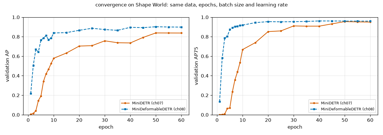
What to read from Figure 8-5 and the table:
- They differ from the start. MiniDETR's AP stays near the floor, at 0.04 or below, through epoch 3. This chapter's model reaches 0.2173 after one epoch and 0.5061 at epoch 2.
- The epoch at which each reaches a given level differs greatly. MiniDETR reached AP 0.5 at epoch 9, this chapter's model at epoch 2. For AP 0.8 it is epoch 50 versus epoch 7. MiniDETR only passed 0.8 after the learning rate was lowered (epoch 48).
- AP is higher at the end too. Final AP is 0.8982, 0.06 higher than Chapter 7's 0.8375. AP75 nearly converges, at 0.9594 versus 0.9500; that is the two curves meeting at the end of the right-hand plot. AP is the average over IoU thresholds 0.5 – 0.95 (Chapter 3), and since AP50 is actually lower and AP75 similar while AP is higher, most of the difference probably comes from thresholds stricter than 0.75 (per-threshold AP was not printed). This means the boxes fit more precisely.
- The curve is not smooth. AP dips and recovers: 0.6698 → 0.6431 from epoch 3 to 4, 0.8109 → 0.7676 from epoch 7 to 8, and 0.8862 → 0.8652 from epoch 25 to 35. With a curve from a single seed, we cannot tell whether these fluctuations are chance.
- The answer to the question left by Chapter 7. Chapter 7 said, "whether the mini DETR's curve was on the slow side, we will judge by comparison in Chapter 8". With the same data and the same training loop, Chapter 7's curve was on the slow side.
- Do not compare training times. 841 seconds and 631 seconds were measured at different times on a GPU shared with other work. They are no basis for saying "Deformable runs faster".
What made it faster?
It is tempting here to write "deformable attention made convergence faster". We cannot write that. Look again at the "What changed from Chapter 7" table. The two models differ in several ways.
- Cross-attention became deformable attention, and queries got reference points.
- Boxes are produced as changes from a reference and refined layer by layer, with separate heads per layer.
- Classification switched to focal loss, prior-probability bias initialization, and sigmoids without ∅, and the matching cost changed.
- The encoder was removed and there are now two feature levels.
What this experiment tells us goes only as far as "the Deformable DETR approach as a whole learned faster than Chapter 7's DETR on this data". How much each part contributes can only be found by removing parts one at a time, and the ablations later do part of that. To give it away: iterative box refinement contributed a lot, and no experiment isolated deformable attention or focal loss on its own.
The paper offers one number useful for this distinction. DETR-DC5+ in Table 1 is DETR-DC5 with focal loss and 300 queries added, and after 50 epochs of training it reaches AP 36.2, not much different from DETR-DC5's 35.3. Deformable DETR at the same 50 epochs reaches 43.8. So on COCO, focal loss and the number of queries alone do not explain the gap. That said, this is the paper's COCO experiment; it does not mean this chapter's shapes-world experiment showed the same thing.
Boxes refined layer by layer
We evaluate the outputs of decoder layers 1, 2, and 3 of the trained main model separately (the same table as in Chapter 7).
[디코더 층별 예측과 중복]
디코더 층 | AP     AP50   AP75  | NMS 뒤 AP  AP50  | 점수≥0.5 예측 수 | 그중 IoU>0.5 로 겹치는 쌍
    1     | 0.7752 0.9536 0.8827 | 0.7734  0.9631 |     1196         |     47
    2     | 0.8820 0.9740 0.9433 | 0.8817  0.9798 |     1208         |     39
    3     | 0.8982 0.9795 0.9594 | 0.8955  0.9803 |     1206         |      9
[박스 반복 정제] 층마다 매칭된 예측 박스와 정답의 평균 IoU: 1층 0.8820, 2층 0.9293, 3층 0.9353
- Figure: Figure 8-6 AP (left) and AP50 (right) per decoder layer of the main model. The solid blue line is without NMS, the dashed orange line after NMS (IoU 0.5). Note the narrow vertical range (AP50 spans 0.95 – 0.98).
- Validation AP and AP50 per decoder layer. AP rises from 0.775 at layer 1 to 0.882 at layer 2 and 0.898 at layer 3, with the before- and after-NMS lines nearly overlapping. With NMS, AP50 rises from 0.954 to 0.963 at layer 1 and is almost unchanged at layer 3.
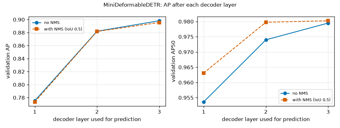
- AP rises substantially across layers: 0.7752 → 0.8820 → 0.8982. Chapter 7's MiniDETR went 0.8067 → 0.8365 → 0.8375. The gain from layer 1 to layer 2 was 0.03 in Chapter 7 and 0.11 here. The mean IoU between matched predicted boxes and ground truth also rises at each layer, 0.8820 → 0.9293 → 0.9353. The structure in which each layer corrects the previous layer's boxes shows in the numbers.
- Layer 1 alone is lower than Chapter 7 (0.7752 vs. 0.8067). This chapter's layer 1 is at a disadvantage: it must produce boxes after a single read with reference points and sampling points that do not depend on the image. This model's good performance comes from refinement in the later layers.
- There are fewer duplicates. In the last layer, among predictions scoring 0.5 or higher, 9 pairs overlap with IoU above 0.5 (45 in Chapter 7). Applying NMS lowers AP slightly, 0.8982 → 0.8955, and AP50 stays almost the same, 0.9795 → 0.9803. Chapter 7's observation that NMS brings no benefit holds here too. At layer 1, NMS raises AP50 from 0.9536 to 0.9631.
- Figure: Figure 8-7 Boxes being refined on validation images #1 (top) and #2 (bottom). Leftmost: the 12 initial reference points (orange stars = queries that end up scoring 0.5 or higher, gray dots = the rest) and ground truth (dashed white). The three columns on the right: the boxes (green) those queries produced after each decoder layer.
- Two validation images. The leftmost column shows the 12 learned reference points and the ground-truth boxes; the other three columns show predicted boxes after decoder layers 1, 2, and 3. The reference points are in the same places in both images; from layer 1 the boxes already enclose the objects, and they snap closer to the dashed ground truth with each layer.
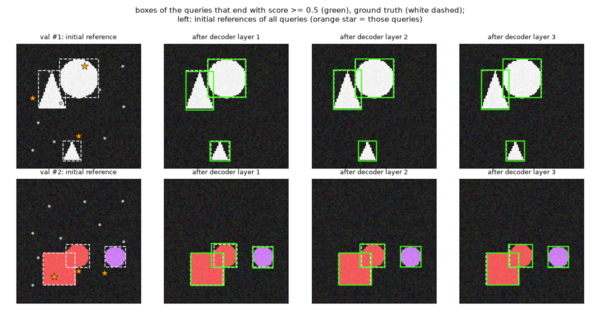
Two things to see in Figure 8-7:
- Reference points are independent of the image. The 12 points in the leftmost column are in the same places in the top and bottom images. The learned reference points printed in the log are spread across the whole image, \(x\) from 0.13 to 0.86 and \(y\) from 0.18 to 0.85. The reference points of queries that end up responsible for objects (orange stars) are generally near the objects but not at their centers, and some stars lie outside the ground-truth boxes. Even so, layer 1 immediately moves the boxes onto the objects.
- Layer 1's boxes are slightly off, and layers 2 and 3 snap them to the ground truth. The visible difference is small: the mean IoU goes from 0.88 to 0.93 – 0.94, and this is what decides AP at high IoU thresholds.
- Figure: Figure 8-8 Predictions (solid green, score 0.5 or higher) and ground truth (dashed white) on validation images 0 – 7. "k pred / m gt" in each title gives the number of predictions and ground-truth objects. These are the same eight images as in Chapter 7's prediction figure.
- Predicted boxes and ground truth on eight validation images. The counts mostly match, with scores between 0.94 and 0.99. The fourth image has two ground-truth objects but one prediction; the triangle was missed.
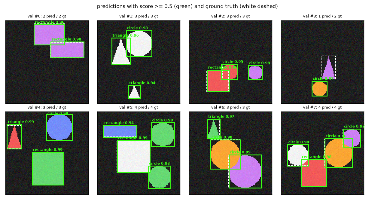
Seven of the eight images in Figure 8-8 have the right count. In #3 the triangle was missed ("1 pred / 2 gt"): its score fell short of 0.5. Chapter 7's model found both in the same image. Note the scores too: 0.94 – 0.99, lower than Chapter 7's, which were nearly 1.00. This difference is revisited in "What did not go as expected" below.
Where the sampling points land
Let us see where the trained model actually reads. For the highest-scoring query on validation image #1 (query 5, responsible for a circle), its 32 sampling points are plotted for each layer.
[표본점] 검증 그림 #1, 질의 5: 층마다 표본점 8×2×2개
  1층 (기준 = 점): 기준에서 가장 먼 표본점까지 0.389 (그림 한 변 = 1), 그림 안에 있는 표본점 비율 0.91, 가장 큰 가중치 0.932 (고르면 0.250), 레벨별 가중치 몫 [0.831 0.169]
  2층 (기준 = 박스): 기준에서 가장 먼 표본점까지 0.161 (그림 한 변 = 1), 그림 안에 있는 표본점 비율 1.00, 가장 큰 가중치 0.892 (고르면 0.250), 레벨별 가중치 몫 [0.867 0.133]
  3층 (기준 = 박스): 기준에서 가장 먼 표본점까지 0.176 (그림 한 변 = 1), 그림 안에 있는 표본점 비율 1.00, 가장 큰 가중치 0.942 (고르면 0.250), 레벨별 가중치 몫 [0.892 0.108]
학습된 기준점 (질의 12개의 x, y): (0.30,0.79) (0.71,0.76) (0.26,0.22) (0.13,0.85) (0.13,0.44) (0.55,0.18) (0.86,0.50) (0.17,0.63) (0.86,0.18) (0.36,0.47) (0.50,0.74) (0.67,0.37)
- Figure: Figure 8-9 The 32 sampling points read at each decoder layer by query 5 (circle, score 0.98) on validation image #1. White star = reference point (for layers 2 and 3, the center of the reference box), dashed white = reference box, yellow = level 0 (12×12), light blue = level 1 (6×6). Circle area is the attention weight.
- Sampling points of the query responsible for the circle, drawn for the three decoder layers. At layer 1 they spread widely around the reference point, with some outside the top of the image. At layers 2 and 3 they gather inside and on the border of the reference box, covering the circle.
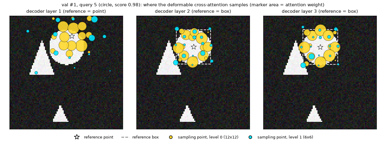
- Layer 1 looks widely. With a point reference, the offsets are in cell units, and the sampling points spread up to 0.389 (39% of the image side) from the reference point. 9% land outside the image and read 0. As noted earlier, the layer-1 sampling points of the one-stage model do not change with the image. This pattern is "where this query looks first, in any image".
- Layers 2 and 3 look according to the box. Once the reference becomes the box produced by the previous layer, the sampling points gather inside and on the border of that box. The distance to the farthest sampling point shrinks to 0.161 and 0.176, and all points are inside the image. This is exactly the equation in which the offset is multiplied by the box size.
- The weights are not uniform. Split evenly across a head's 4 sampling points (2 levels × 2 points), each would get 0.25, but some heads give 0.93 – 0.94 to a single point. This is far from the "all equal" of initialization.
- The weight goes to the fine level. Level 0 gets 83 – 89% and level 1 gets 11 – 17%.
This figure is an example from one image and one query. Do not generalize it to "deformable attention always looks like this". The paper plots the sampling points of a model trained on COCO (Appendix A.6) and explains that the decoder attends to the whole foreground object, not just its extremities, with sampling points and weights adapted to the object's size and shape.
Ablations
We remove or change one component and retrain from scratch. To save time, a short 15-epoch schedule was used (learning rate ×1/10 after epoch 12). Do not compare these directly with the main model's numbers (60 epochs). The baseline is the first row (base), retrained with the same 15 epochs.
[절제 요약] 에폭 15 뒤의 검증 성능 (시드 1개)
설정                      | AP     AP50   AP75  | 1층만의 AP  AP75 | AP≥0.8 첫 에폭 | 학습 시간
refine, 2 levels (base)   | 0.8763 0.9768 0.9395 | 0.7202   0.8297 |        7       |   131초
no box refinement         | 0.7500 0.9461 0.8599 | 0.7040   0.8048 |     None       |   181초
two-stage                 | 0.9100 0.9921 0.9747 | 0.8864   0.9665 |        6       |   205초
single level (12x12)      | 0.8563 0.9639 0.9288 | 0.7061   0.8130 |        8       |   156초
+ 3 encoder layers        | 0.8720 0.9776 0.9395 | 0.7364   0.8403 |        7       |   213초
[2단계] 디코더를 거치기 전, 선택된 제안 12개만으로 채점한 AP (검증 앞 250장): AP 0.8330, AP50 0.9898, AP75 0.9664
| Row | What changed |
| refine, 2 levels (base) | Same settings as the main model (iterative box refinement, 2 levels, one-stage, no encoder) |
| no box refinement | Iterative box refinement off: every layer uses the initial reference point and they share one head |
| two-stage | Two-stage query selection on: the initial references are proposal boxes selected from the image |
| single level (12x12) | Level 1 (6×6) removed, only level 0 used. 16 sampling points per query |
| + 3 encoder layers | Chapter 7's 3-layer global self-attention encoder added before the decoder |
- Figure: Figure 8-10 Validation AP (left) and AP75 (right) for the five ablation settings, 15 epochs each, one seed.
- Validation AP and AP75 curves for the five ablation settings. Only the setting without box refinement is clearly below the rest; two-stage is on top from the start, and the other three stay close together.
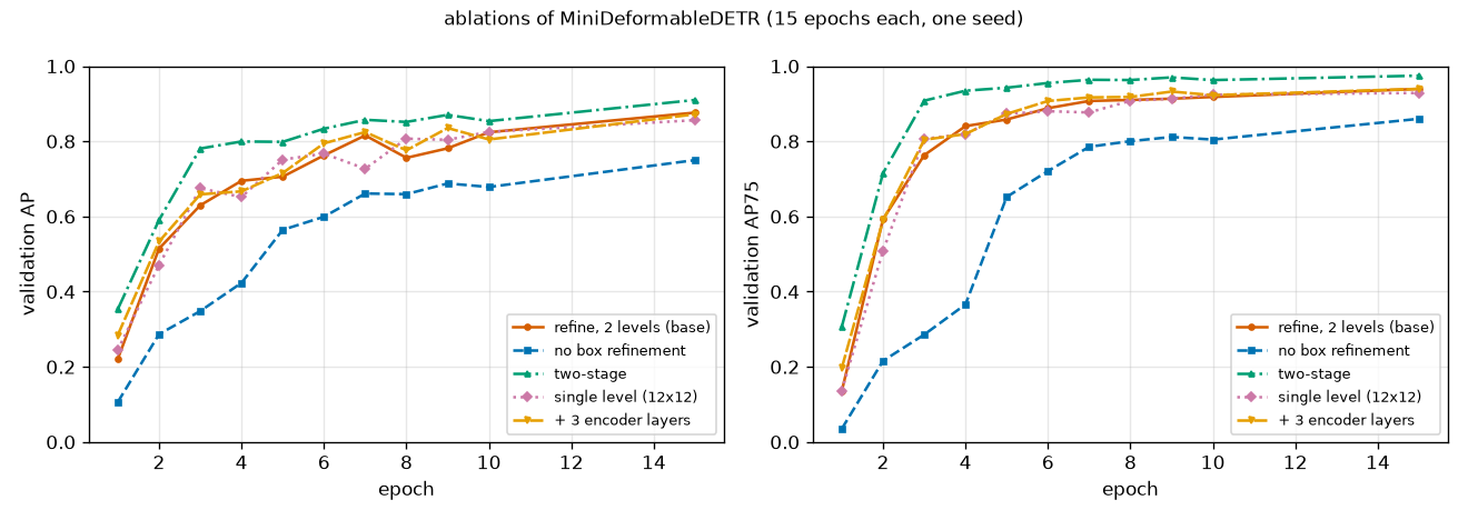
- Caution: a single seed
- Each setting was trained only once. Even the main model and base, which share the same settings, have slightly different early curves (AP at epoch 1 is 0.2173 vs. 0.2206, at epoch 3 0.6698 vs. 0.6297), due to nondeterminism in GPU operations. So differences of around ±0.02 may be chance. Below, "there is a difference" is claimed only for the two rows that clearly separate across the whole curve. The "학습 시간" (training time) column was also measured on a shared GPU and cannot be used to compare speed between settings.
- Removing iterative box refinement makes things clearly worse. AP 0.8763 → 0.7500. In Figure 8-10 only this setting (dashed blue) stays below from start to finish, and it did not reach AP 0.8 within 15 epochs. Layer-1-only AP is similar, 0.7202 vs. 0.7040; the gap opens in the later layers. With refinement, AP rises from 0.72 at layer 1 to 0.88 at the last layer; without it, it only rises from 0.70 to 0.75. Note, however, that this row removes more than refinement: separate per-layer heads and the later layers' deformable attention using the box as reference are removed too.
- Two-stage was best. AP 0.9100, higher even than the main model trained for 60 epochs (0.8982). Its curve is on top from epoch 1. Its layer-1-only AP is 0.8864: when references are chosen from the image, boxes are good from the first layer.
- Reducing to one level is slightly lower (0.8563). A difference of 0.02 may be within chance. Shape sizes span a narrow range, 0.14 – 0.42 of the image side, and are much larger than one cell of the 12×12 map, so multi-scale may have had little to do on this data. We cannot say this experiment reproduced the multi-scale gain the paper saw on COCO (for small objects).
- Adding 3 encoder layers changed nothing (0.8720). This means the fact that Chapter 7's MiniDETR has an encoder and this chapter's model does not did not, at least on this chapter's side, determine performance.
Chapter 7's MiniDETR had AP 0.6327 at epoch 15. Even the setting without refinement (0.7500) is higher. But the two runs used different learning rate schedules (the ablations lower it after epoch 12, Chapter 7 after epoch 48), so this is not a rigorous comparison. It should be read only as a hint that "even without refinement it is faster than DETR".
Evaluating the proposals alone
Look at the last line of the ablation output. It is the score of the two-stage model before the decoder, using only the boxes and scores of the 12 selected proposals (first 250 validation images): AP 0.8330, AP50 0.9898, AP75 0.9664. Without a decoder, just a head producing one box per cell is already a usable detector (the 0.9100 after the decoder is over all 500 images, so the two should not simply be subtracted).
- Figure: Figure 8-11 Figure 8-7 for the two-stage model. Leftmost: among the 12 selected proposals, the boxes (orange) and centers (orange stars) of those that end up scoring 0.5 or higher, the centers of the other proposals (gray dots), and the ground truth (dashed white). The three columns on the right: boxes after each decoder layer (green).
- Two validation images for the two-stage model. In the leftmost column the selected proposal boxes already enclose the objects, and the boxes after the decoder layers are almost the same.
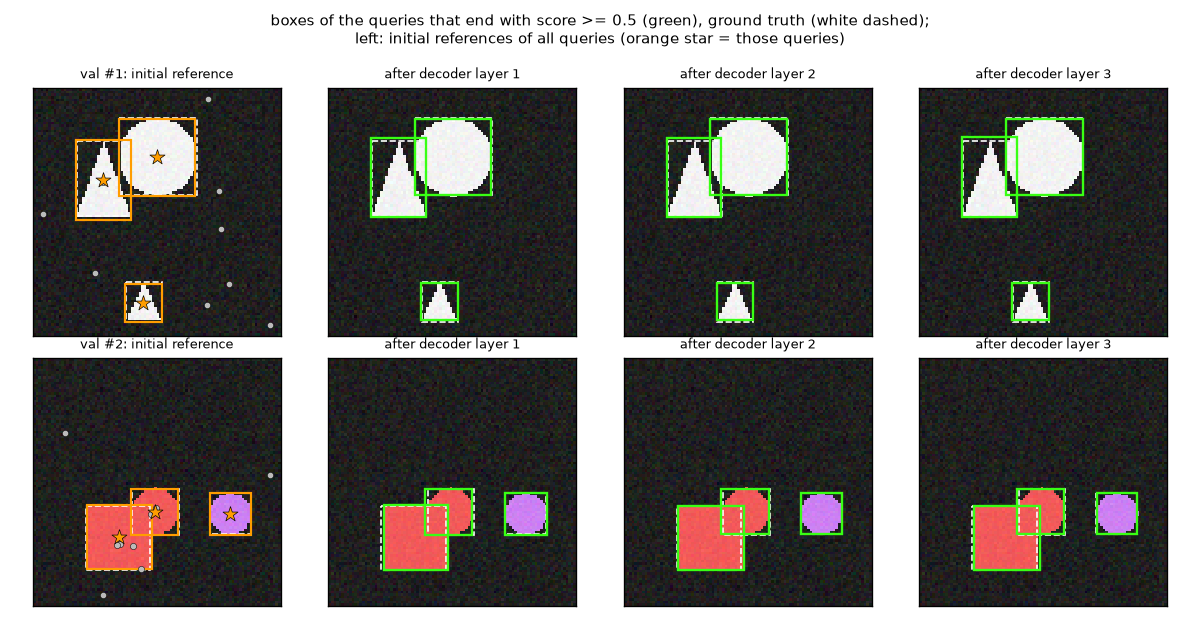
Compare Figure 8-11 side by side with Figure 8-7. The one-stage model's initial references were points independent of the image. The two-stage model's initial references are boxes that already enclose the objects, and they differ per image. The decoder's job is to polish them slightly and keep only one of the proposals crowding onto the same object (a few gray dots are inside objects; these are proposals that ended up scoring below 0.5, probably pointing at the same object).
This result benefits from the circumstances of this data. The backbone built in Chapter 7 has a receptive field (the input area seen by one output cell) of 43 pixels, which covers the largest shape, so a single cell's features already contain information about the whole object. This does not mean proposals alone would do this well on COCO. Still, the direction matches the paper. In Table 1 of the paper, the two-stage variant has AP 0.8 higher than the model with iterative refinement alone (45.4 → 46.2). RF-DETR uses this two-stage query selection by default.
What did not go as expected
To avoid reading only the good numbers, here is what in this experiment went against expectations or could not be explained.
- Chapter 7's DETR has higher AP50. Final AP50 is 0.9863 for Chapter 7 and 0.9795 here, while AP and AP75 are higher here. In other words, this chapter's model was better at "fitting boxes precisely", while in this experiment Chapter 7's model was slightly ahead at "finding every object and outputting it with the right class and ranking". The number of predictions scoring 0.5 or higher points the same way: there are 1,265 ground-truth objects, and this chapter's model output 1,206 while Chapter 7's output 1,290. This means more objects were missed or given low scores, the triangle missed in #3 of Figure 8-8 being one example. The cause was not analyzed. Plausible candidates are the tendency of scores trained with focal loss to come out low, the fixed reference points of the 12 queries, and post-processing that allows one query to be selected under two classes. The two-stage model, with AP50 0.9921, does not show this gap.
- Faster convergence cannot be attributed to deformable attention alone. As noted, several things changed together, and in the ablations the largest contribution came from iterative box refinement.
- On a 12×12 map, deformable attention was not fast. One cross-attention took 2.6× as long as ordinary attention. The benefit appears with large maps.
- No effect of multi-scale or the encoder was visible. The differences are within the chance range (±0.02).
- A connection to Chapter 4's experiment. In Chapter 4's imbalanced classification experiment, focal loss did not always win either. The effect of changing a single loss depends on the task and settings, and this chapter did not measure it separately.
What the paper reported
To keep them separate from the mini experiments, here are the numbers the paper reported on COCO (Deformable DETR paper, Table 1, ResNet-50 backbone, COCO 2017 validation set).
| Model | Epochs | AP | AP50 | AP75 | APS (small objects) | Training GPU hours | Inference FPS |
| Faster R-CNN + FPN | 109 | 42.0 | 62.1 | 45.5 | 26.6 | 380 | 26 |
| DETR | 500 | 42.0 | 62.4 | 44.2 | 20.5 | 2000 | 28 |
| DETR-DC5 | 500 | 43.3 | 63.1 | 45.9 | 22.5 | 7000 | 12 |
| DETR-DC5 | 50 | 35.3 | 55.7 | 36.8 | 15.2 | 700 | 12 |
| DETR-DC5+ (focal loss, 300 queries) | 50 | 36.2 | 57.0 | 37.4 | 16.3 | 700 | 12 |
| Deformable DETR | 50 | 43.8 | 62.6 | 47.7 | 26.4 | 325 | 19 |
| + iterative box refinement | 50 | 45.4 | 64.7 | 49.0 | 26.8 | 325 | 19 |
| ++ two-stage | 50 | 46.2 | 65.2 | 50.0 | 28.8 | 340 | 19 |
- Epochs. Deformable DETR reaches AP 43.8 in 50 epochs, surpassing DETR (42.0) and DETR-DC5 (43.3) trained for 500 epochs. In the paper's words, "better performance with 10× fewer training epochs". DETR-DC5 trained for the same 50 epochs reaches only 35.3.
- Small objects. Small-object AP rises from DETR's 20.5 to 26.4, close to Faster R-CNN + FPN (26.6), which uses multi-scale features.
- Refinement and two-stage. Iterative box refinement adds 1.6 AP (43.8 → 45.4), and two-stage adds another 0.8 (→ 46.2).
- Speed. Inference runs at 19 images per second, faster than DETR-DC5 (12) and slower than DETR (28), which uses a single feature map, and Faster R-CNN + FPN (26).
Compared with this chapter's mini experiments, "high AP in few epochs", "the gain from refinement", and "the gain from two-stage" pointed the same way. "Strong on small objects" and "the gain from multi-scale" could not be confirmed in the shapes world. And the tenfold gap of 500 versus 50 epochs in the paper belongs to COCO; in the shapes world, even Chapter 7's DETR reached AP 0.84 in 60 epochs.
Summary
- The Deformable DETR paper traces DETR's slow convergence and weakness on small objects to the way attention handles feature maps. At first it looks at all cells almost uniformly (\(\approx 1/N_k\)), and the cost of encoder self-attention is quadratic in the number of cells, so large maps are out of reach.
- Deformable attention reads only \(M \cdot L \cdot K\) sampling points around each query's reference point \(p_q\). The offsets \(\Delta p\) and weights \(A\) are predicted from the query vector \(z_q\) by linear layers, with no dot product with keys.
- Bilinear interpolation is a weighted average of four neighbors: the weights are \((1 - t_x)(1 - t_y)\), \(t_x(1 - t_y)\), \((1 - t_x)t_y\), \(t_x t_y\) and sum to 1. The cell grid is \(u_x = xW - 0.5\) (
align_corners=False), and outside the map is 0. - The value read is differentiable with respect to the sampling location: \(\partial v / \partial x = W[(1 - t_y)(v_{01} - v_{00}) + t_y(v_{11} - v_{10})]\). That is why offsets can be learned by gradient descent without ground truth. The gradient sees only four neighbors.
- With a point reference, the offset unit is a cell of that level (\(\Delta p / (W_l, H_l)\)); with a box reference, it is \(1/K\) of half the box size (\(\Delta p / K \cdot (w, h)/2\)). Weights are softmaxed over \(L \cdot K\) points per head. Initially, \(k\) cells in eight directions, with weights \(1/(LK)\).
- The (query, position) pairs read drop from \(N_q \cdot HW\) to \(N_q \cdot MLK\), but the value projection is still applied to every cell. In this chapter's measurements, deformable attention was actually slower on small maps and overtook on large maps.
- Boxes are corrected from a reference: \(\hat{b}^{d} = \sigma(\Delta b^{d} + \sigma^{-1}(\operatorname{sg}(\hat{b}^{d-1})))\), \(\sigma^{-1}(x) = \log\frac{x}{1-x}\). Adding in logit space keeps them within 0 – 1, and the gradient is cut when passing to the next layer.
- Classification uses per-class sigmoids without ∅ and focal loss; the matching classification cost is "loss if treated as positive − loss if treated as negative", and the full cost is \(2\,C_{\text{cls}} + 5\,\lVert \hat{b}_i - b_j \rVert_1 - 2\,\operatorname{GIoU}\).
- In two-stage query selection, every cell produces a proposal box (starting at the cell center with size \(0.05 \cdot 2^{l}\)) and a score, and the top \(N\) become the decoder's reference boxes.
- In the shapes world, this chapter's model learned much faster than Chapter 7's (7 epochs vs. 50 epochs to AP 0.8) and reached a higher final AP (0.898 vs. 0.838). But this cannot be attributed to deformable attention alone, and Chapter 7 had higher AP50. In the ablations, the differences from iterative box refinement and two-stage were clear (one seed).
DETR turned detection into set prediction, and Deformable DETR turned that into a model that learns quickly and can afford large feature maps. Deformable attention that reads only around a reference point, boxes corrected from a reference, and queries chosen by looking at the image were all inherited by RF-DETR's decoder, each in a slightly altered form. What remains is speed. The paper's Deformable DETR runs at 19 images per second, still far from real time. Chapter 9 is about making this lineage fast: how RT-DETR turned the DETR family into real-time detectors, and how LW-DETR, with a ViT backbone, window attention, and a shallow deformable decoder, built the direct skeleton of RF-DETR.
Review questions
- 1. Bilinear interpolation by hand — A 2×2 feature map has values \((0,\ 10)\) in row 0 and \((20,\ 40)\) in row 1. Find the value read at point \((x, y) = (0.4,\ 0.7)\), and check that the four weights sum to 1.
- \(u_x = 0.4 \times 2 - 0.5 = 0.3\) and \(u_y = 0.7 \times 2 - 0.5 = 0.9\), so the top-left neighbor is (row 0, column 0), with \(t_x = 0.3\), \(t_y = 0.9\).
- The weights are \(0.7 \times 0.1 = 0.07\), \(0.3 \times 0.1 = 0.03\), \(0.7 \times 0.9 = 0.63\), \(0.3 \times 0.9 = 0.27\), summing to 1.
- The value is \(0.07 \times 0 + 0.03 \times 10 + 0.63 \times 20 + 0.27 \times 40 = 0 + 0.3 + 12.6 + 10.8 = 23.7\).
- 2. Gradient with respect to the sampling location — In the setting of question 1, find \(\partial v / \partial x\) and \(\partial v / \partial y\). Use the gradient to estimate the value read if the sampling point moves \(0.01\) in the \(x\) direction.
- \(\partial v / \partial x = W\,[(1 - t_y)(v_{01} - v_{00}) + t_y(v_{11} - v_{10})] = 2 \times [0.1 \times 10 + 0.9 \times 20] = 2 \times 19 = 38\).
- \(\partial v / \partial y = H\,[(1 - t_x)(v_{10} - v_{00}) + t_x(v_{11} - v_{01})] = 2 \times [0.7 \times 20 + 0.3 \times 30] = 2 \times 23 = 46\).
- Moving \(x\) by \(0.01\) gives \(23.7 + 38 \times 0.01 = 24.08\). Since the interpolation formula is linear in \(t_x\), this estimate is exact within the same four neighbors.
- 3. Coordinate convention — When the normalized coordinate \((0.5,\ 0.5)\) is read on (a) a 3×3 feature map and (b) a 12×12 feature map, which cells are used, and with what weights?
- (a) \(u_x = u_y = 0.5 \times 3 - 0.5 = 1.0\). This is exactly the center of cell (row 1, column 1), so \(t_x = t_y = 0\) and that cell's value comes out unchanged with weight 1. For the map in the text, that is 5.
- (b) \(u_x = u_y = 0.5 \times 12 - 0.5 = 5.5\). This is midway between columns 5 and 6 and rows 5 and 6, so \(t_x = t_y = 0.5\), and the four cells (5, 5), (5, 6), (6, 5), (6, 6) are used with weight \(0.25\) each.
- With an odd number of cells, the image center is a cell center; with an even number, it is the corner where four cells meet. Treating "normalized coordinate × \(W\)" as the column index without subtracting 0.5 puts you off by half a cell.
- 4. Sampling point positions — The offset is \(\Delta p = (2,\ -1)\). (a) With a point reference \((0.30,\ 0.60)\), find the sampling points at the 12×12 level and the 6×6 level. (b) With a box reference \((c_x, c_y, w, h) = (0.30,\ 0.60,\ 0.20,\ 0.40)\) and \(K = 4\), find the sampling point.
- (a) 12×12: \((0.30 + 2/12,\ 0.60 - 1/12) = (0.4667,\ 0.5167)\). 6×6: \((0.30 + 2/6,\ 0.60 - 1/6) = (0.6333,\ 0.4333)\). The same offset goes twice as far on the coarser level.
- (b) \(\big(0.30 + \tfrac{2}{4} \times \tfrac{0.20}{2},\ \ 0.60 - \tfrac{1}{4} \times \tfrac{0.40}{2}\big) = (0.30 + 0.05,\ 0.60 - 0.05) = (0.35,\ 0.55)\). It does not depend on the level size, and if the box doubles in size, the sampling point moves twice as far from the center.
- 5. Counting operations — RF-DETR Medium uses resolution 576, patch size 16, and 300 queries, and its decoder cross-attention uses 16 heads, 1 level, and 2 sampling points. Find (a) the number of cells in the feature map, (b) the number of (query, position) pairs ordinary cross-attention would read at once, and (c) the number of pairs deformable attention reads and the ratio. (d) With the paper's defaults \(M = 8\), \(L = 4\), \(K = 4\), how many outputs does the linear layer producing offsets have?
- (a) \(576 / 16 = 36\), so \(36 \times 36 = 1{,}296\) cells.
- (b) \(300 \times 1{,}296 = 388{,}800\) pairs.
- (c) \(300 \times 16 \times 1 \times 2 = 9{,}600\) pairs. The ratio is \(388{,}800 / 9{,}600 = 40.5\)×. As seen in the text, though, this is a ratio of "positions read", not of total multiplications or actual time.
- (d) \(2MLK = 2 \times 8 \times 4 \times 4 = 256\) (the weight layer has \(MLK = 128\)).
- 6. Inverse sigmoid and box refinement — A reference box has center \(x\) coordinate \(0.25\), and the box head output \(\Delta b_x = 0.4\). (a) Find the new coordinate (\(\log 3 = 1.0986\), \(e^{0.6986} = 2.0110\)). (b) What must \(\Delta b_x\) be to move the coordinate to exactly \(0.5\)?
- (a) \(\sigma^{-1}(0.25) = \log\frac{0.25}{0.75} = -\log 3 = -1.0986\). Adding gives \(-1.0986 + 0.4 = -0.6986\). \(\sigma(-0.6986) = \frac{1}{1 + e^{0.6986}} = \frac{1}{3.0110} = 0.3321\).
- (b) We need \(\sigma^{-1}(0.5) = 0\), so \(\Delta b_x = 0 - (-1.0986) = 1.0986\). In terms of odds, this turns \(1/3\) into \(1\), i.e., triples it (\(= e^{1.0986}\)).
- 7. Focal matching cost — A prediction gives probability \(\hat{p} = 0.5\) to the ground-truth class entry. With \(\alpha = 0.25\), \(\gamma = 2\), find the classification cost \(C_{\text{cls}}\) (\(-\log 0.5 = 0.6931\)). Compared with another prediction with \(\hat{p} = 0.9\) (\(-1.3986\) in the text), which does matching choose if the box costs are equal?
- Loss if treated as positive: \(0.25 \times 0.5^2 \times 0.6931 = 0.0433\). Loss if treated as negative: \(0.75 \times 0.5^2 \times 0.6931 = 0.1300\).
- \(C_{\text{cls}} = 0.0433 - 0.1300 = -0.0866\) (computed from the unrounded values \(0.04332 - 0.12997\)).
- It chooses the prediction with \(\hat{p} = 0.9\) (\(-1.3986\)), which has the smaller cost. In the full cost, this difference is multiplied by the coefficient 2.
- 8. What the experiment can tell us — This chapter's model reached AP 0.8 in 7 epochs, while Chapter 7's MiniDETR took 50. Explain why this result alone does not support the conclusion "deformable attention speeds up convergence", and propose one experiment that would test that claim directly.
- Because several things changed between the two models. Besides the type of cross-attention, box prediction relative to a reference with per-layer refinement, separate per-layer heads, focal loss with prior-probability bias initialization, sigmoid classification without ∅ and its matching cost, the presence of an encoder, and the number of feature levels all changed together. In the ablations, removing iterative box refinement alone dropped 15-epoch AP from 0.8763 to 0.7500, so a large share of the fast convergence may lie elsewhere than deformable attention. On top of that, there is only one seed.
- To test it, compare two models that differ in only one thing. For example, train Chapter 7's MiniDETR with only the classification changed to focal loss and sigmoids to measure the loss's share (DETR-DC5+ in Table 1 of the paper is this kind of experiment), or train this chapter's model with only the cross-attention reverted to ordinary attention, keeping the rest (box prediction from a reference, focal loss), and compare. Either way, multiple seeds are needed.
See also
Favorite site
- 08. Deformable DETR: Looking Only Where It Matters
- ch08_deformable.py - hands-on code for this chapter
- Deformable DETR: Deformable Transformers for End-to-End Object Detection (Zhu et al., ICLR 2021)
- Deformable Convolutional Networks (Dai et al., 2017)