RF-DETR:Tutorial:07-DETR
lastmod 2026-11-18created 2026-11-183 edits
DETR: Detection as Set Prediction is Chapter 7 of the RF-DETR tutorial and the first chapter of Part 2 (the DETR lineage). It brings together all the parts built so far (boxes (Chapter 2), scoring (Chapter 3), the classification loss (Chapter 4), attention (Chapter 5) and the backbone (Chapter 6)) to build the first detector. The idea behind DETR is "a detector's answer is a set, so train it to output the set directly." The chapter follows the Hungarian matching and set loss that make this work all the way through, with equations and hand calculations, and then trains a mini DETR from scratch in the shape world to check whether NMS is really unnecessary. RF-DETR keeps the skeleton from this chapter, and Deformable DETR in the next chapter addresses this chapter's limitations (slow convergence and a cost that grows quadratically with resolution).
Topics covered: what must change to detect without anchors and NMS (the set prediction view); a fixed number \(N\) of prediction slots and "no object (∅)"; bipartite matching and the Hungarian algorithm; the three terms of DETR's matching cost and why the classification term uses probabilities rather than log probabilities; the set loss (Hungarian loss) and a hand calculation of the loss for one image; how one-to-one matching removes duplicate predictions; the DETR architecture (CNN backbone → encoder → decoder → heads) with object queries, parallel decoding and auxiliary losses; and finally the mini DETR's training curve, query specialization, cross-attention, per-layer AP, the NMS experiment, and the limitations of DETR.
- Original: 07. DETR: Detection as Set Prediction
- Practice code:
code/ch07_detr.py(brute-force matching,HungarianMatcher,SetCriterion,MiniDETR, the training loop and post-processing). It trains for 60 epochs (7,500 steps) on 4,000 shape-world images, which takes about 15 minutes on a laptop GPU;--quickis a 2-epoch reduced version for catching errors (about ten-odd seconds on a CPU). Reading time for the original is about 100 minutes; difficulty ★★★★☆. - Previous: 06. Vision Transformer and DINOv2 / Next: 08. Deformable DETR: Looking Only Where Needed
- Notation in this chapter
- \(N\): the number of object queries (prediction slots). In Chapter 5 it was the number of tokens, but in this chapter it is always the number of queries. The DETR paper uses 100; the mini model in this chapter uses 12.
- \(T\): the number of ground-truth objects in one image. Always \(T \le N\). (Chapter 2 wrote the number of ground truths as \(M\), but from Chapter 5 onward \(M\) denotes the bundle of image tokens produced by the encoder, so here we use \(T\), as in the code.)
- \(K\): the number of classes (3 in the shape world). The "no object" class is written \(\varnothing\) and occupies the last slot of the logits (index \(K\)). So the classification output has \(K + 1\) entries.
- \(i\): the index of a prediction (query); \(j\): the index of a ground truth. To match the code, counting starts at 0. "Prediction 1" is the second prediction.
- \(\hat{p}_i(c)\): the probability that prediction \(i\) assigns to class \(c\) ("p-hat"). \(\hat{b}_i\): the box of prediction \(i\). Symbols with a hat (^) are model predictions; those without (\(c_j\), \(b_j\)) are ground truth. All boxes are normalized \((c_x, c_y, w, h)\).
- \(C\): the cost matrix, of shape \((N, T)\). \(C_{ij}\) is the cost of assigning prediction \(i\) to ground truth \(j\). In Chapter 2 \(C\) was the enclosing box, but in this chapter it is used only for the cost matrix.
- \(\sigma\) ("sigma"): an assignment. \(\sigma(j)\) is the index of the prediction paired with ground truth \(j\). Because it is the same letter as the sigmoid \(\sigma(\cdot)\) from Chapter 4, this chapter does not write the sigmoid as a formula and only mentions it in words.
- \(B\): batch size, \(D\): model dimension, \(H \times W\): height and width of the feature map, \(L\): the number of decoder layers.
Can we get rid of the hand-crafted components?
Anchors and NMS revisited
Chapter 1 surveyed the detectors that came before DETR. Those detectors lay thousands to tens of thousands of candidate locations (anchors, grid cells, region proposals) over the image and ask at each one, "Is there an object here, and if so, how much should the box be adjusted?" Human-designed rules creep into this approach in two places.
- During training: which location is responsible for which ground truth. This is decided by rules such as "every anchor whose IoU with a ground-truth box exceeds a threshold is responsible for that ground truth." Since several locations share one ground truth, a well-trained detector outputs several similar boxes for a single object. These are the duplicate predictions seen in Chapter 3.
- During inference: how duplicates are removed. The NMS (non-maximum suppression) from Chapter 3 walks through predictions in score order and removes those that overlap heavily. This adds one more knob, the IoU threshold, and as Chapter 3 showed, it can remove real objects that sit close together.
The anchor sizes and aspect ratios, the rules that assign ground truths, and the NMS threshold are all set by hand rather than learned from data. The DETR paper calls these "hand-designed components that explicitly encode prior knowledge about the task" and points out that a detector's performance depends heavily on how they are designed.
Changing the question
Why do duplicates arise? Because of the training rule "several locations share one ground truth." So the question can be changed as follows.
- The question of this chapter
- Can a model be trained to produce exactly one prediction per object? Then there would be no duplicates to remove, so NMS would be unnecessary, and there would be no need to lay candidate locations densely, so anchors would be unnecessary too.
DETR (DEtection TRansformer) from 2020 (Carion et al., "End-to-End Object Detection with Transformers", ECCV 2020) is the model that answered this question. The answer has two ingredients. One is a loss that pairs predictions with ground truths one to one; the other is a Transformer architecture in which predictions can see each other. Feed in an image and the final answer comes out directly without hand-crafted post-processing, and the loss computed from that answer is backpropagated in one pass from start to finish. This approach is called end-to-end detection.
Set prediction
A fixed number of slots and "no object"
As Chapter 1 said, a detector's answer is a set of (class, box) pairs. The number of elements differs from image to image, and the elements have no order. A neural network outputs tensors of fixed size, so it cannot directly output "a set whose size varies each time." DETR solves this problem very simply.
- Keep a fixed number \(N\) of prediction positions. These are called prediction slots. Each slot produces one (class probabilities, box) pair.
- Choose \(N\) comfortably larger than the number of objects that can appear in one image. The DETR paper used \(N = 100\) for COCO (7 objects per image on average, at most 63 in the training set), and the mini model for the shape world (1 – 4 objects per image) uses \(N = 12\).
- With more slots than objects, some slots are left over. The leftover slots are made to answer "no object." This is the background class \(\varnothing\) seen in Chapter 4. With \(K\) classes, the classification output has \(K + 1\) entries.
This makes the output shape fixed regardless of the image: classification logits (B, N, K+1) and boxes (B, N, 4). For an image with 2 objects, 2 of the 12 slots answer with objects and 10 answer ∅. The problem of "outputting, in one go, a set made of a fixed number of elements" is called set prediction.
- Analogy
- Suppose a restaurant has 12 servers. Guests (objects) arrive 1 – 4 parties at a time. In a good restaurant, exactly one server attends each party and the rest wait as "no party assigned." Two servers attending the same party and placing the same order twice (a duplicate prediction) is not acceptable, and neither is a party left with no server (a miss). DETR's approach is not to have a person decide who takes which party, but to let the servers look at each other and split the work on their own.
What produces the slots is the object query previewed in Chapter 5. An object query is a learned vector tasked with "go find one object." \(N\) of them enter the decoder and become \(N\) output vectors, and each output vector becomes the prediction of one slot. The architecture is covered in detail in the DETR architecture section later. For now, read it as "query \(i\) = slot \(i\) = prediction \(i\)."
Comparing unordered sets
Now for training. The model has produced \(N\) predictions, and there are \(T\) ground truths. To compute a loss, we must decide "which prediction to compare with which ground truth." For a classifier there is nothing to think about: there is one output and one ground truth. In detection, however, this is not fixed.
- Ground truths have no order. Whether the circle or the triangle is listed first in the annotation file, it is the same ground truth.
- Slots have no fixed duties either. No person sets a convention such as "slot 0 is the leftmost object" (if one did, that would be yet another hand-crafted rule).
What happens if we pair them by index, "compare prediction \(i\) with ground truth \(i\)"? A large loss appears when the predictions match the ground truths exactly in content but come out in a different order. The model would have to solve a problem it does not need to solve (guessing the line order of the annotation file). So a set prediction loss must give the same value no matter how the predictions are ordered. This property is called permutation invariance (Chapter 5's permutation equivariance meant "shuffle the input and the output is shuffled the same way," while permutation invariance means "shuffle it and the value stays the same").
DETR's solution is this: before computing the loss, look at the current predictions and first find the best-matching pairs. The prediction that best matches ground truth \(j\) becomes its partner, but no prediction may be the partner of two ground truths. Once the pairs are fixed, the rest is ordinary loss computation. This "pair finding" is the bipartite matching of the next section.
Bipartite matching
The cost matrix and assignments
Let us write pair finding as a problem. The ingredient is a single table. For every pair of prediction \(i\) and ground truth \(j\), a table recording as a number "how poorly these two match if paired" is called the cost matrix, written \(C\). Its shape is \((N, T)\), and the smaller \(C_{ij}\) is, the better prediction \(i\) matches ground truth \(j\).
Choosing one prediction for each ground truth is called an assignment, written \(\sigma\). \(\sigma(j)\) is the index of the prediction paired with ground truth \(j\). There is one condition.
\(j \ne j' \;\Rightarrow\; \sigma(j) \ne \sigma(j') \qquad \text{(different ground truths are paired with different predictions)}\)
That is, one prediction per ground truth, and at most one ground truth per prediction. This is one-to-one matching. The total cost of an assignment is the sum of the costs of the paired cells, and what we want is the assignment \(\hat{\sigma}\) ("sigma-hat") with the smallest total cost.
\(\hat{\sigma} = \operatorname{arg\,min}_{\sigma} \sum_{j=0}^{T-1} C_{\sigma(j),\, j}\)
\(\operatorname{arg\,min}_{\sigma}\) means "the \(\sigma\) that makes the following value smallest." Since this is the problem of lining up predictions on one side and ground truths on the other and choosing lines that connect the two sides, it is called bipartite matching ("bipartite" means the points split into two groups and lines run only between groups). In mathematics it has long been studied under the name assignment problem.
- Comparing with the paper's notation
- Equation (1) of the DETR paper is \(\hat{\sigma} = \operatorname{arg\,min}_{\sigma \in \mathfrak{S}_N} \sum_{i}^{N} \mathcal{L}_{\text{match}}(y_i, \hat{y}_{\sigma(i)})\). The paper pads the ground-truth set with \(\varnothing\) to size \(N\) and then finds the minimum over permutations of \(N\) elements (\(\mathfrak{S}_N\) is the set of all such permutations). In the paper, \(i\) is the index of a ground truth and \(\sigma(i)\) is the index of its paired prediction. This chapter writes the ground-truth index as \(j\) only to match the rows and columns of the cost matrix; it is the same equation. As the paper says, the cost against a ground truth padded with \(\varnothing\) is a constant independent of the prediction, so only the partners of the \(T\) real ground truths need to be determined. This point is used again a little later.
Solving by hand: trying all twenty-four
Let us solve a small example by hand. The image has 4 predictions (\(N = 4\)) and 3 ground truths (\(T = 3\): circle, circle, triangle). Suppose the cost matrix is as follows. (Where these numbers come from is computed in the next section, DETR's matching cost. It is the same example used by toy_example in the practice code.)
| \(C_{ij}\) | GT 0 (circle) | GT 1 (circle) | GT 2 (triangle) |
| Prediction 0 | −1.3618 | −0.2609 | 5.5975 |
| Prediction 1 | −0.2370 | 2.2602 | 6.8998 |
| Prediction 2 | 5.8077 | 4.2476 | −1.4608 |
| Prediction 3 | 4.3247 | 1.8215 | 3.7627 |
Negative costs are nothing strange. A cost only expresses the ordering "smaller means a better match," so it may be below 0. We write an assignment as (partner of GT 0, partner of GT 1, partner of GT 2). For example, \((1, 0, 2)\) means GT 0 ↔ prediction 1, GT 1 ↔ prediction 0, GT 2 ↔ prediction 2. There are 4 ways to choose the partner of GT 0, 3 remaining ways for GT 1, and 2 remaining ways for GT 2, so there are \(4 \times 3 \times 2 = 24\) assignments in total. Computing all of them and sorting by total cost gives the following.
| Rank | Assignment | Total cost | Rank | Assignment | Total cost | Rank | Assignment | Total cost |
| 1 | (1, 0, 2) | −1.9587 | 9 | (0, 2, 3) | 6.6485 | 17 | (2, 1, 3) | 11.8307 |
| 2 | (0, 3, 2) | −1.0011 | 10 | (1, 3, 0) | 7.1820 | 18 | (3, 1, 0) | 12.1825 |
| 3 | (0, 1, 2) | −0.5624 | 11 | (0, 3, 1) | 7.3595 | 19 | (2, 0, 1) | 12.4466 |
| 4 | (1, 3, 2) | 0.1237 | 12 | (1, 2, 3) | 7.7734 | 20 | (2, 3, 0) | 13.2268 |
| 5 | (3, 0, 2) | 2.6030 | 13 | (2, 0, 3) | 9.3096 | 21 | (2, 1, 0) | 13.6655 |
| 6 | (1, 0, 3) | 3.2648 | 14 | (1, 2, 0) | 9.6082 | 22 | (3, 2, 0) | 14.1699 |
| 7 | (0, 1, 3) | 4.6611 | 15 | (0, 2, 1) | 9.7856 | 23 | (2, 3, 1) | 14.5290 |
| 8 | (3, 1, 2) | 5.1242 | 16 | (3, 0, 1) | 10.9636 | 24 | (3, 2, 1) | 15.4722 |
(These values were computed the same way as brute_force_assignment in the practice code and are given to four decimal places.) Let us check the top row by hand.
- Total cost of the optimal assignment (1, 0, 2)
- \(C_{1,0} = -0.2370, \qquad C_{0,1} = -0.2609, \qquad C_{2,2} = -1.4608\)
- The assignment \((1, 0, 2)\) is \(\sigma(0) = 1\), \(\sigma(1) = 0\), \(\sigma(2) = 2\). Read the three cells from the table in (row = prediction, column = ground truth) order.
- Add the three cells. No total cost among the 24 is smaller than this. Prediction 3 is not paired with any ground truth, and it will later learn "no object."
The optimal assignment for the hand-calculated example is as follows (Figure 7-1 in the original). On the left are the 4 predictions (queries); on the right are the 3 ground truths and ∅. The parentheses show the class each prediction gave the highest probability and that probability, and the costs \(C_{ij}\) are rounded.
- Prediction 1 (circle 0.60) — GT 0 (circle): cost −0.24
- Prediction 0 (circle 0.70) — GT 1 (circle): cost −0.26
- Prediction 2 (triangle 0.60) — GT 2 (triangle): cost −1.46
- Prediction 3 (∅ 0.80): no partner. It is connected to ∅ by a dotted line and learns ∅.
The total cost is \(-0.24 - 0.26 - 1.46 = -1.96\), the minimum among the 24. Each ground truth has exactly one line, and each prediction has at most one.
There are two things to read from the figure. First, predictions 0 and 1 both answered "circle," and both boxes are near GT 0 (checked in the next section). Even so, the two cannot share GT 0. Second, the lines therefore cross. Prediction 0 gave up GT 0, its own best match (\(-1.36\)), to prediction 1 and went to GT 1. Why that is better overall is the next topic.
Why greedy assignment fails
Is there an easier way than trying all 24? The first idea that comes to mind is "starting from GT 0, give each ground truth the cheapest of the remaining predictions." Grabbing whatever looks best at the moment like this is called greedy assignment. Applied to the table above, it goes like this.
- Following greedy assignment
- \(\text{GT 0:}\quad \min(-1.3618,\; -0.2370,\; 5.8077,\; 4.3247) = -1.3618 \;\Rightarrow\; \text{prediction 0}\)
- The smallest value in the GT 0 column is prediction 0. Prediction 0 can no longer be used.
- The smallest value in the GT 1 column after excluding prediction 0 (\(-0.2609\)). GT 0 has already taken prediction 0, the only one that matched GT 1 reasonably well.
- Choose between the remaining predictions 1 and 2.
- The total cost of the greedy assignment \((0, 3, 2)\) is \(-1.0011\), rank 2 in the table. It is \(0.9576\) worse than the optimum.
Where was the loss incurred? It becomes clear when GT 0 and GT 1 are looked at in isolation. Greedy produced \(-1.3618 + 1.8215 = 0.4597\), while the optimum produced \(-0.2370 - 0.2609 = -0.4979\). Prediction 0 is useful for both GT 0 and GT 1, but prediction 1 is useful only for GT 0 (\(2.2602\) against GT 1). So it is better to give prediction 1, which is useful in only one place, to GT 0, and move the versatile prediction 0 to GT 1. This answer cannot be found by looking at one cell; it only emerges from looking at the whole table. That is why the assignment problem is harder than "picking the minimum in each column separately."
The combinatorial explosion
Then why not always try everything? Let us count the assignments.
- Number of assignments with \(N\) predictions and \(T\) ground truths
- \(N \times (N-1) \times (N-2) \times \cdots \times (N-T+1)\)
- The partner of GT 0 can be chosen in \(N\) ways, the partner of GT 1 in the remaining \(N - 1\) ways, …, and the partner of the last ground truth \(T - 1\) in the remaining \(N - T + 1\) ways. Since the choices are made in sequence, multiply.
- \(N! = N \times (N-1) \times \cdots \times 1\) is "\(N\) factorial." Dividing out the trailing \((N-T)!\) part of \(N!\) leaves only the product of the first \(T\) factors.
- This is the example above. It equals the number of rows in the table.
| Case | \(N\) | \(T\) | Number of assignments \(N!/(N-T)!\) |
| Hand-calculated example | 4 | 3 | 24 |
| This chapter's mini DETR, image with 4 objects | 12 | 4 | \(12 \times 11 \times 10 \times 9 = 11{,}880\) |
| DETR (\(N = 100\)), 7 objects (the COCO average) | 100 | 7 | \(80{,}678{,}106{,}432{,}000 \approx 8.1 \times 10^{13}\) |
| DETR (\(N = 100\)), 20 objects | 100 | 20 | \(\approx 1.3 \times 10^{39}\) |
Even with a computer that evaluates a billion (\(10^{9}\)) assignments per second, matching a single image with 7 objects would take \(8.1 \times 10^{13} / 10^{9} \approx 80{,}678\) seconds, a little over 22 hours. With 20 objects it would take \(1.3 \times 10^{30}\) seconds, more than \(10^{22}\) years. Training must do this matching at every step for every image. Trying everything (brute-force search) is usable only at toy sizes.
The intuition behind the Hungarian algorithm
Fortunately, the exact optimal assignment for this problem can be found without trying everything. The classic method is the Hungarian algorithm (Kuhn, 1955). Its running time grows only with roughly the cube of the matrix's side length, so for \(N = 100\) it takes a little over \(100^3 = 10^{6}\) operations, incomparably smaller than \(10^{39}\). Because DETR finds its pairs this way, the pairing is called Hungarian matching.
Covering the full algorithm with proofs is beyond the scope of this tutorial. Here we check just one idea underlying it, using a small example with a square matrix. The idea is this.
- Key observation
- In a square cost matrix, subtracting the same number from every cell of one row (or one column) does not change the optimal assignment. Every assignment uses exactly one cell in that row, so the total cost of every assignment drops by the same amount and the ranking stays the same.
Using this observation, we reshape the matrix into one with "many zeros." If every cell is at least 0 and an assignment can be completed using only zero cells, that assignment's total cost is 0; no total cost can be below 0, so it is optimal. Let us try it on an example that gives 3 jobs (columns) to 3 workers (rows), one each.
- 3×3 example — subtracting from rows and columns
- \(A = \begin{pmatrix} 4 & 1 & 3 \\ 2 & 0 & 5 \\ 3 & 2 & 2 \end{pmatrix}\)
- The starting matrix. \(A_{ij}\) is the cost for worker \(i\) to take job \(j\). There are \(3! = 6\) assignments.
- Subtract each row's minimum (1, 0, 2) from that row. Now every row has at least one zero. The total subtracted is \(1 + 0 + 2 = 3\).
- Subtract each column's minimum (1, 0, 0) from that column. Now every column has a zero too. The total subtracted so far is \(3 + 1 = 4\).
- Check whether an assignment can be completed using only zeros. The zeros of worker 0 and worker 1 are both only in job 1. The two cannot take the same job, so not yet.
- Create more zeros. Subtract 1 from rows 0 and 1, which lack zeros (1 is the smallest nonzero cell in these two rows), and add 1 to column 1, which would otherwise become \(-1\), to bring it back to 0 or above. We only subtracted from rows and added to a column, so the optimal assignment is still the same. The total subtracted is \(4 + 1 + 1 - 1 = 5\).
- Now the zero cells \((0,1), (1,0), (2,2)\) complete an assignment. Its total cost in the original matrix is 5, equal to the total subtracted so far, 5. Trying all six gives total costs of 6, 11, 5, 7, 9 and 6, confirming that 5 is the minimum.
The Hungarian algorithm systematically repeats the work of "checking whether an assignment can be completed with zeros alone and, if not, deciding which rows to subtract from and which columns to add to." The rules for that decision and the proof that the repetition always terminates are the heart of the algorithm, which we do not cover here. We need only two facts: the answer it finds is exactly optimal, and it is fast.
- When there are more predictions than ground truths
- Our cost matrix is \((N, T)\), not square. In that case only subtracting from columns is safe. Every assignment uses each column (ground truth) exactly once, but some rows (predictions) go unused, so "every assignment uses one cell in that row" does not hold. The simplest fix, as in the paper, is to append \(N - T\) dummy columns whose costs are all 0 to make an \(N \times N\) square. A dummy column means "paired with ∅," and since its cost is a constant (0) independent of the prediction, it does not affect the partners of the real ground truths. Seen this way an assignment becomes a permutation of \(N\) elements, giving \(N!\) of them, but the \((N - T)!\) ways of permuting the dummy columns among themselves are the same assignment, so the number of distinct ones is the \(N!/(N-T)!\) counted earlier.
Checking brute force against SciPy
In practice we do not implement it ourselves but use SciPy's scipy.optimize.linear_sum_assignment(cost). It accepts a rectangular matrix as is and returns (row indices, column indices) of the assignment with the minimum total cost. RF-DETR's public code (matcher.py) also solves the matching with this function.
- Note — the algorithm inside SciPy
- The documentation for SciPy 1.18, used in this chapter, says the function is implemented with "a modified Jonker – Volgenant algorithm." It is a different (faster) algorithm that solves the same problem and produces the same minimum total cost as the Hungarian algorithm. Because the DETR paper wrote that it "computes it with the Hungarian algorithm," in this lineage it is called Hungarian matching whatever solver is used. What matters to us is not the solver's internals but the promise that it "returns the optimal one-to-one assignment."
Rather than just trusting that promise, let us verify it. The practice code includes a brute-force search over all assignments and a greedy assignment.
def brute_force_assignment(cost: np.ndarray):
    """비용 행렬에서 총비용이 가장 작은 일대일 배정을 "전부 해 보고" 찾는다.

    cost: (N, T) — cost[i, j] 는 예측 i 를 정답 j 에 배정하는 비용. N ≥ T (예측이 정답보다 많다).
    정답 0, 1, …, T−1 에 서로 다른 예측을 하나씩 고르는 방법은 N·(N−1)·…·(N−T+1) 가지다.
    돌려주는 값: (정답 j 가 짝지어진 예측 번호의 튜플, 그 총비용, 훑어본 배정의 수).
    N = 100, T = 20 이면 약 10^39 가지라 이 방법은 쓸 수 없다 → 헝가리안 알고리즘이 필요한 이유.
    """
    num_preds, num_targets = cost.shape
    best_rows, best_cost, tried = None, float("inf"), 0
    for rows in itertools.permutations(range(num_preds), num_targets):  # rows[j] = 정답 j 의 짝
        total = sum(cost[rows[j], j] for j in range(num_targets))
        tried += 1
        if total < best_cost:
            best_rows, best_cost = rows, total
    return best_rows, float(best_cost), tried

def greedy_assignment(cost: np.ndarray):
    """비교용 탐욕 배정: 정답 0 부터 차례로, 아직 안 쓰인 예측 가운데 비용이 가장 작은 것을 고른다.

    빠르지만 총비용이 최소라는 보장이 없다 (앞의 정답이 뒤의 정답에게 더 필요한 예측을 가져갈 수 있다).
    """
    used, rows = set(), []
    for j in range(cost.shape[1]):
        order = [i for i in np.argsort(cost[:, j]) if i not in used]
        rows.append(int(order[0]))
        used.add(int(order[0]))
    return tuple(rows), float(sum(cost[rows[j], j] for j in range(cost.shape[1])))
itertools.permutations(range(N), T) yields, one after another, every way of "choosing \(T\) of \(N\) in order," that is, all \(N!/(N-T)!\) assignments. The output of applying all three methods to the cost matrix above is as follows (it is the first part printed when this chapter's practice file is run; the full run is in the Reading the results section later).
무차별 탐색: 배정 24가지 가운데 최소 — 정답 0,1,2 의 짝 = 예측 (1, 0, 2), 총비용 -1.9587
scipy linear_sum_assignment: 예측 (1, 0, 2), 총비용 -1.9587
탐욕 배정(정답 0 부터 가장 싼 예측): 예측 (0, 3, 2), 총비용 -1.0011
check 무차별 탐색 = scipy: True
check 무작위 6×T 비용 행렬 200개: 최소 비용의 최대 차이 = 8.88e-16
This agrees with the answer found by hand. The last line is a check added because a single example is not convincing. On 200 randomly generated \(6 \times T\) cost matrices (\(T\) from 1 to 4), the brute-force minimum total cost was compared with SciPy's total cost, and the largest difference was \(8.88 \times 10^{-16}\) (the level of 64-bit floating-point rounding error). SciPy found the true minimum in all 200.
DETR's matching cost
Definitions of the three terms
Now it is time to see where the numbers in the cost matrix come from. "How poorly prediction \(i\) and ground truth \(j\) match" requires looking at two things together: whether the class is right and whether the boxes are close. DETR's matching cost is the sum of three terms.
\(C_{ij} \;=\; \underbrace{-\,\hat{p}_i(c_j)}_{\text{class}} \;+\; \lambda_{\text{L1}}\,\underbrace{\lVert \hat{b}_i - b_j \rVert_1}_{\text{L1 distance}} \;+\; \lambda_{\operatorname{GIoU}}\,\underbrace{\big(-\operatorname{GIoU}(\hat{b}_i, b_j)\big)}_{\text{overlap}}, \qquad \lambda_{\text{L1}} = 5, \quad \lambda_{\operatorname{GIoU}} = 2\)
- Class term \(-\hat{p}_i(c_j)\). The softmax probability that prediction \(i\) gave to the class \(c_j\) of ground truth \(j\), with a negative sign. The more probability given to the correct class, the smaller the cost. It ranges from \(-1\) to \(0\).
- L1 term. The L1 distance from Chapter 2: the sum of the absolute differences of the four numbers \((c_x, c_y, w, h)\).
- GIoU term. The GIoU from Chapter 2 with a negative sign. A larger GIoU means better overlap (from \(-1\) to \(1\)), so flipping the sign turns it into a cost where "smaller is better."
The coefficients \(\lambda_{\text{L1}} = 5\) and \(\lambda_{\operatorname{GIoU}} = 2\) are the values from Appendix A.4 of the DETR paper (the paper writes the latter as \(\lambda_{\text{iou}}\)), and the class term's coefficient is 1. These are the same coefficients as the box loss \(\mathcal{L}_{\text{box}}\) at the end of Chapter 2. Writing out the three terms for the hand-calculated example separately gives the following (exactly as output by the practice code).
[손계산 예] 예측 4개 × 정답 3개 (정답: 원, 원, 삼각형)
C_cls = −p̂_i(c_j)
 [[-0.7  -0.7  -0.1 ]
 [-0.6  -0.6  -0.1 ]
 [-0.1  -0.1  -0.6 ]
 [-0.05 -0.05 -0.1 ]]
C_L1 = ‖b̂_i − b_j‖₁
 [[0.12 0.24 0.86]
 [0.18 0.54 1.08]
 [0.9  0.66 0.08]
 [0.8  0.44 0.7 ]]
C_GIoU = −GIoU
 [[-0.6309 -0.3805  0.6988]
 [-0.2685  0.0801  0.7999]
 [ 0.7039  0.5238 -0.6304]
 [ 0.1874 -0.1642  0.1814]]
C = 1·C_cls + 5·C_L1 + 2·C_GIoU
 [[-1.3618 -0.2609  5.5975]
 [-0.237   2.2602  6.8998]
 [ 5.8077  4.2476 -1.4608]
 [ 4.3247  1.8215  3.7627]]
All four matrices have shape (number of predictions, number of ground truths) \(= (4, 3)\). In the mini DETR it is \((12, T)\) per image, and with the DETR paper's settings it would be \((100, T)\). The predictions and ground truths in this example are as follows.
| Class probabilities [circle, square, triangle, ∅] | Box \((c_x, c_y, w, h)\) | |
| Prediction 0 | [0.70, 0.10, 0.10, 0.10] | (0.33, 0.31, 0.24, 0.24) |
| Prediction 1 | [0.60, 0.20, 0.10, 0.10] | (0.24, 0.26, 0.16, 0.16) |
| Prediction 2 | [0.10, 0.20, 0.60, 0.10] | (0.66, 0.70, 0.30, 0.24) |
| Prediction 3 | [0.05, 0.05, 0.10, 0.80] | (0.50, 0.50, 0.40, 0.40) |
| GT 0 | Circle | (0.30, 0.30, 0.20, 0.20) |
| GT 1 | Circle | (0.42, 0.34, 0.30, 0.30) |
| GT 2 | Triangle | (0.70, 0.70, 0.30, 0.20) |
The first two columns of \(C_{\text{cls}}\) are identical because GT 0 and GT 1 are the same class (circle). The class alone cannot tell the two circles apart; the box terms do.
Computing one cell by hand
Let us compute from scratch the cell \(C_{1,0}\) (prediction 1 and GT 0) used in the optimal assignment. GIoU is computed after converting to the corner representation, in the same order as in Chapter 2.
- Computing \(C_{1,0}\)
- \(-\hat{p}_1(c_0) = -\hat{p}_1(\text{circle}) = -0.60\)
- The class term. The class of GT 0 is circle, and prediction 1 gave circle a probability of 0.60.
- The L1 term. Subtract matching components of \((c_x, c_y, w, h)\) and add the absolute values.
- Convert the center representation to the corner representation \((x_1, y_1, x_2, y_2)\) by subtracting and adding half the width and height from the center.
- The left and top of the intersection rectangle are the larger of the two boxes' values (\(0.20, 0.20\)); the right and bottom are the smaller (\(0.32, 0.34\)).
- Inclusion–exclusion: add the two areas and subtract the overlap once.
- The smallest box containing both boxes. Use the smaller values for left and top and the larger values for right and bottom.
- GIoU is IoU minus "the fraction of the enclosing box not covered by the two boxes" (Chapter 2).
- Add the three terms with their coefficients. This equals \(-0.237\), the first cell of the second row of \(C\) in the output.
Computing prediction 0 against GT 0 the same way gives \(-0.70 + 5 \times 0.12 - 2 \times 0.6309 = -1.3618\). Prediction 0 matches GT 0 much better than prediction 1 does (its box is closer and its probability higher). The reason the optimal assignment still gave GT 0 to prediction 1 was shown earlier: prediction 0 was the only candidate that could also take GT 1.
- Difference from the paper's formula — one constant
- The paper writes the box part of the matching cost the same way as the loss, \(\mathcal{L}_{\text{box}} = \lambda_{\text{iou}}\,(1 - \operatorname{GIoU}) + \lambda_{\text{L1}} \lVert \cdot \rVert_1\). This chapter's code (and RF-DETR's public code) uses \(-\operatorname{GIoU}\) instead of \(1 - \operatorname{GIoU}\). The difference is a constant \(\lambda_{\operatorname{GIoU}} \times 1 = 2\) per cell. Every assignment uses exactly \(T\) cells, so the total cost of every assignment shifts by the same \(2T\), and the optimal assignment is the same. In this example, the minimum total cost computed with the paper's formula is \(-1.9587 + 2 \times 3 = 4.0413\), and the assignment is still \((1, 0, 2)\).
Why probabilities rather than log probabilities
In Chapter 4 the classification loss was \(-\log \hat{p}\). The class term of the matching cost, however, is \(-\hat{p}\) without the log. The paper explains that the matching cost uses probabilities instead of log probabilities because this makes the class term commensurable with the box term \(\mathcal{L}_{\text{box}}\), and that it also gave better results in experiments. The numbers make the meaning clear.
| Probability given to the correct class \(\hat{p}\) | 0.9 | 0.5 | 0.1 | 0.01 | 0.001 |
| \(-\hat{p}\) (DETR's matching cost) | −0.9 | −0.5 | −0.1 | −0.01 | −0.001 |
| \(-\log \hat{p}\) (if the log were used) | 0.105 | 0.693 | 2.303 | 4.605 | 6.908 |
- \(-\hat{p}\) always lies between \(-1\) and \(0\). The difference in class cost between two predictions is at most 1.
- \(-\log \hat{p}\) grows without bound as the probability approaches 0. At \(\hat{p} = 0.001\) it is 6.9.
- What about the box side? In the hand-calculated example, \(5 \times C_{\text{L1}}\) lies between 0.4 and 5.4, and \(2 \times C_{\operatorname{GIoU}}\) between \(-1.26\) and \(1.60\). By definition the GIoU term cannot leave the range \(-2\) to \(2\).
With probabilities, all three terms are bounded and can be compared with each other. With the log, the class term alone can grow without bound, so early in training, when the model barely knows the classes, a prediction whose "box is nearly exact but whose probability is very low" is easily pushed out of the matching. That last sentence is this tutorial's interpretation; the paper gives only the reasons above (matching the scale and better experimental results).
From Deformable DETR onward, classification switches to per-class sigmoids and the focal loss, and the class term of the matching changes to a focal-loss form as well (Chapter 8). The practice code's HungarianMatcher already accepts class_cost="focal" for that purpose. This chapter uses only "prob".
Matching has no gradient
The output of matching is indices, such as "GT 0's partner is prediction 1." Indices are integers; a tiny change to the predictions usually leaves them unchanged until, at some point, they abruptly switch to different indices. For such values, the gradient learned in Chapter 4 (how much something changes when the input changes slightly) is undefined. So matching is done outside gradient computation. In PyTorch this is @torch.no_grad().
- Matching only decides who pairs with whom. The values of the cost matrix themselves do not enter the loss.
- Once the pairs are fixed, they are treated as given constants and the loss is computed. Gradients flow only through that loss.
- Matching is done afresh at every step for every image. As training progresses and predictions change, the pairs can change too. A query that handled an object yesterday may handle ∅ today.
Set loss
The Hungarian loss formula
With the pairs fixed, compute the loss. First, set a target class \(t_i\) for each query.
\(t_i = \begin{cases} c_j & \text{when prediction } i \text{ is the partner of GT } j \text{ } \big(i = \hat{\sigma}(j)\big) \\ \varnothing & \text{when prediction } i \text{ has no partner} \end{cases}\)
Then Equation (2) of the DETR paper, the set loss, reads as follows in this chapter's notation. The paper calls it the Hungarian loss.
\(\mathcal{L}_{\text{Hungarian}} \;=\; \underbrace{\sum_{i=0}^{N-1} -\log \hat{p}_i(t_i)}_{\text{classification of all queries}} \;+\; \underbrace{\sum_{j=0}^{T-1} \mathcal{L}_{\text{box}}\big(b_j,\, \hat{b}_{\hat{\sigma}(j)}\big)}_{\text{boxes of matched queries}}\)
- The classification term applies to all \(N\) queries. Matched queries must predict the ground-truth class, and unmatched ones must predict \(\varnothing\). It is exactly the softmax cross-entropy (CE) of Chapter 4.
- The box term applies only to the \(T\) matched queries. Unmatched queries have no ground-truth box to compare against, so there is no loss wherever their boxes are.
- The box loss is Chapter 2's \(\mathcal{L}_{\text{box}}(b, \hat{b}) = \lambda_{\text{L1}} \lVert b - \hat{b} \rVert_1 + \lambda_{\operatorname{GIoU}}\,(1 - \operatorname{GIoU}(b, \hat{b}))\) with coefficients 5 and 2. Here it is \(1 - \operatorname{GIoU}\) (so that the loss is at least 0).
The matching cost and the loss look alike but are different things. Placing them side by side makes the difference clear.
| Matching cost \(C_{ij}\) | Set loss | |
| Role | Decides who pairs with whom | Trains the model with the fixed pairs |
| Scope of computation | All pairs \((N, T)\) | Matched pairs only (\(T\) pairs) + classification over all \(N\) |
| Class term | \(-\hat{p}_i(c_j)\) (probability) | \(-\log \hat{p}_i(t_i)\) (log probability) |
| Box term | \(5 \cdot \text{L1} - 2 \cdot \operatorname{GIoU}\) | \(5 \cdot \text{L1} + 2 \cdot (1 - \operatorname{GIoU})\) |
| Handling of ∅ | Does not appear (constant) | Target class of unmatched queries |
| Gradient | None ( | Yes (backpropagation) |
Why "no object" is down-weighted
Using the formula above as is has one problem: the target of most queries is \(\varnothing\).
- With the DETR paper's settings (\(N = 100\), an average of 7 objects per COCO image), 93 of the 100 classification terms say "predict ∅."
- For this chapter's mini model (\(N = 12\)), the 500 validation images contain 1,265 ground truths, so on average 2.53 per image are objects and 9.47 are ∅.
This is the class imbalance seen in Chapter 4. Left alone, simply answering "always ∅" removes most of the classification loss, so the model drifts in that direction. DETR's remedy is simple: multiply terms whose target is ∅ by a weight of 0.1. In the paper's words, "we down-weight the log-probability term when \(c_i = \varnothing\) by a factor 10 to account for class imbalance," and it adds that this plays the same role as Faster R-CNN's subsampling of proposals to balance positives and negatives.
Counting the "loudness" after weighting, in the paper's setting the ∅ side is \(93 \times 0.1 = 9.3\) and the object side \(7 \times 1 = 7\), roughly equal. In the mini model, the ∅ side is \(9.47 \times 0.1 = 0.947\) and the object side \(2.53\). If Chapter 4's focal loss is a refined remedy that "reduces the loss of easy examples," this is a crude remedy that "reduces the loss of ∅ wholesale." From Chapter 8 onward it is replaced by the focal loss family.
Normalization: the paper's formula versus the implementation
Equation (2) is written as a sum, but a sum varies in size with the batch size and number of objects, so in practice it is divided. Precisely, this chapter's implementation (SetCriterion) computes the following three terms. \(T_{\text{batch}}\) is the number of ground-truth objects in the whole batch, \(w(c)\) is the class weight (0.1 for \(\varnothing\), 1 otherwise), and the sums run over all images in the batch.
\(\mathcal{L}_{\text{cls}} = \frac{\sum_{i} w(t_i)\,\big(-\log \hat{p}_i(t_i)\big)}{\sum_{i} w(t_i)}, \qquad \mathcal{L}_{\text{L1}} = \frac{1}{T_{\text{batch}}} \sum_{j} \lVert b_j - \hat{b}_{\hat{\sigma}(j)} \rVert_1, \qquad \mathcal{L}_{\operatorname{GIoU}} = \frac{1}{T_{\text{batch}}} \sum_{j} \Big(1 - \operatorname{GIoU}\big(b_j, \hat{b}_{\hat{\sigma}(j)}\big)\Big)\)
\(\mathcal{L} = 1 \cdot \mathcal{L}_{\text{cls}} + 5 \cdot \mathcal{L}_{\text{L1}} + 2 \cdot \mathcal{L}_{\operatorname{GIoU}}\)
- The denominator of the classification loss is not "the number of objects"
- Appendix A.2 of the paper says "all losses are normalized by the number of objects inside the batch." This chapter's implementation does exactly that for the two box-loss terms (dividing by \(T_{\text{batch}}\), clamped to at least 1 so that a batch with no objects does not divide by 0). The classification loss, however, uses PyTorch's
F.cross_entropy(..., weight=...), which divides the weighted sum by the sum of the weights (a weighted mean). So the denominator is not \(T_{\text{batch}}\) but \(T_{\text{batch}} + 0.1 \times (\text{number of queries whose target is ∅})\). DETR's public code is known to use this function as well, but the repository was not available in the environment where this tutorial was made, so this could not be checked directly. The two approaches differ only slightly in the size of the classification loss (0.4518 versus 0.4669 in the hand calculation below); the intent, "scale the ∅ terms down by a factor of 10," is the same.
Computing the loss of one image all the way through
Returning to the hand-calculated example, we compute the loss all the way through for the optimal assignment \((1, 0, 2)\). There is one image, so \(T_{\text{batch}} = 3\).
- Classification loss
- \(t_0 = c_1 = \text{circle}, \qquad t_1 = c_0 = \text{circle}, \qquad t_2 = c_2 = \text{triangle}, \qquad t_3 = \varnothing\)
- Set the target class for each query. Prediction 0's partner is GT 1, prediction 1's is GT 0, prediction 2's is GT 2, and prediction 3 has no partner.
- The negative log (natural log) of the probability each query gave its target class. Prediction 0 gave 0.70 to circle, prediction 1 gave 0.60 to circle, prediction 2 gave 0.60 to triangle, and prediction 3 gave 0.80 to ∅.
- Multiply by the weights and add. Only the term for prediction 3, whose target is ∅, is scaled by 0.1, giving \(0.0223\).
- The sum of the weights.
- The weighted mean. Dividing by the number of objects, 3, would have given \(1.4006 / 3 = 0.4669\).
- Box loss and total
- \(\lVert b_0 - \hat{b}_1 \rVert_1 = 0.18, \qquad \lVert b_1 - \hat{b}_0 \rVert_1 = 0.09 + 0.03 + 0.06 + 0.06 = 0.24, \qquad \lVert b_2 - \hat{b}_2 \rVert_1 = 0.04 + 0 + 0 + 0.04 = 0.08\)
- The L1 distance for each pair. The first value was computed earlier; the others are obtained the same way from the boxes in the table. They can also be read from cells \((1,0)\), \((0,1)\) and \((2,2)\) of \(C_{\text{L1}}\) in the output.
- Divide the sum over the three pairs by the number of objects, 3.
- \(1 - \operatorname{GIoU}\) for each pair. The GIoU values are read from the same three cells of \(C_{\operatorname{GIoU}}\) in the output with the sign flipped.
- Divide the sum over the three pairs by the number of objects.
- Multiply the three terms by their coefficients and add (the middle two products use the unrounded \(0.5/3\) and \(1.7206/3\)).
The practice code's output gives the same values.
손실: loss_ce 0.4518, loss_bbox 0.1667, loss_giou 0.5735 → 전체 1·ce + 5·bbox + 2·giou = 2.4322
질의별 목표 클래스: ['circle', 'circle', 'triangle', 'no-object'] −log p̂: [0.3567 0.5108 0.5108 0.2231] 가중치: [1.  1.  1.  0.1]
check 가중 교차 엔트로피 손계산 0.451820 vs SetCriterion 0.451819
There is something to read in these numbers. Of the total 2.43, the GIoU term is 1.15, the L1 term 0.83 and the classification term 0.45. In this example, the box side makes up most of the loss. Also, although prediction 3 gave only 0.80 to ∅, it added just 0.0223 to the classification loss, because of the 0.1 weight. Prediction 3's box \((0.50, 0.50, 0.40, 0.40)\) was not used anywhere.
Why duplicate predictions disappear
Now back to this chapter's opening question. Why does training with this loss leave only one prediction per object? Let us work through one situation with numbers. Suppose queries A and B both output nearly the same box on one circle, and both answer "circle 0.90, ∅ 0.05." Under Chapter 3's scoring, one would be a true positive and the other a false positive (a duplicate prediction).
- Matching. There is one ground truth, so one-to-one matching takes only the one with even slightly lower cost, say A, as the partner. B has no partner.
- A's loss. The target is circle. The classification term is small, \(-\log 0.90 = 0.105\), and the box loss pulls the box to be more precise. A is rewarded.
- B's loss. The target is ∅. B gave ∅ only 0.05, so the classification term is \(0.1 \times (-\log 0.05) = 0.1 \times 2.996 = 0.300\). Had B given ∅ 0.90, it would have been \(0.1 \times 0.105 = 0.011\). B is penalized even though it was just as accurate.
In other words, as long as two queries both point at the same object with high scores, one of them is bound to receive a gradient saying "you should have answered ∅." The state with the smallest loss is the one in which exactly one query per object gives a high score and all the others answer ∅. In effect, Chapter 3's scoring rule "each ground truth is used only once" has been turned into a training rule. What NMS did in Chapter 3 after the output came out, DETR builds into the model through training.
There is one condition, though. B must be able to know that "A has taken this circle." If the queries answered by looking only at the image, without seeing each other at all, A and B would have no way of deciding who should back off. The channel for this is the decoder's self-attention (Chapter 5). In each decoder layer the queries look at each other's states and negotiate "that query is already pointing at the object, so I'll go to ∅." The DETR paper explains that because the Transformer's self-attention models all pairwise interactions between elements, it is particularly well suited to set prediction constraints such as removing duplicate predictions.
- Only the score is penalized
- Unmatched queries have no box loss. So B's box overlapping A's is not penalized in itself; only B's score being high is. Even in a well-trained DETR, low-score predictions may still sit on top of objects. As the experiment in Chapter 3 showed, low-score duplicates barely reduce AP, so that is enough. Keep this in mind when the later experiment counts "whether duplicates are exactly 0."
DETR architecture
Overall flow and tensor shapes
With the loss settled, let us look at the model trained with it. As the paper says, the architecture is surprisingly simple, with only three parts: a CNN backbone that extracts features from the image, a Transformer encoder and decoder, and small heads that make the final predictions. All the parts were built in Chapters 4 – 5.
This chapter's mini DETR is connected as follows (Figure 7-2 in the original). Parentheses give the tensor shape after passing through each part.
- Image
(B, 3, 96, 96)→ CNN backbone →(B, 128, 12, 12) - 1×1 convolution and flatten →
(B, 144, 128) - Encoder × 3 →
(B, 144, 128). A sinusoidal positional encoding(144, 128)is added to the attention queries and keys in every layer (not to the values). - Decoder × 3: the input is zeros
(B, 12, 128), and the learned object queries(12, 128)and positional encoding are added in every layer →(B, 12, 128) - Classification head → \(K + 1 = 4\) logits per query
(B, 12, 4); box head → 4 values \((c_x, c_y, w, h)\) passed through a sigmoid(B, 12, 4)
It has the same layout as Figure 2 of the DETR paper, only smaller.
Following the figure from left to right, we point out where the shapes change. The right column lists the paper's settings alongside (the paper's values are taken from Sections 3.2 and 4 and Appendix A.4 of the DETR paper).
| Stage | Role | This chapter's mini DETR | DETR paper (ResNet-50) |
| Input | Image | | \((3, H_0, W_0)\), shorter side 480 – 800 pixels |
| Backbone | A CNN extracts features while reducing resolution | 6 layers of 3×3 convolution, stride 8 → | ResNet-50, stride 32 → \((2048, H_0/32, W_0/32)\) |
| 1×1 convolution | Sets the number of channels to the model dimension \(D\) | 128 → 128, | 2048 → 256 |
| Flatten | Turns the grid into one row of tokens (row-major) | | \((HW, 256)\) |
| Positional encoding | 2D sinusoidal (fixed) | | \((HW, 256)\) |
| Encoder | Self-attention among image tokens → FFN | 3 layers, 8 heads, FFN 256 → | 6 layers, 8 heads |
| Object queries | Learned positional embedding | | \((100, 256)\), \(N = 100\) |
| Decoder | Self-attention → cross-attention → FFN | 3 layers → | 6 layers → \((100, 256)\) |
| Classification head | A single linear layer | | \((100, K + 1)\) |
| Box head | 3-layer MLP (hidden size \(D\), ReLU) → sigmoid | | \((100, 4)\) |
| Dropout | 0 | 0.1 | |
| Parameters | 1,333,608 | 41.3 million (ResNet-50 23.5 million + Transformer 17.8 million) |
- Backbone. A stack of the convolutions from Chapter 4. Passing through three stride-2 layers reduces the size \(96 \to 48 \to 24 \to 12\). The paper's ResNet-50 has stride 32, but applied as is to a 96-pixel image it would leave only a \(3 \times 3\) grid, so the stride was reduced to 8.
- 1×1 convolution and flatten. A 1×1 convolution mixes only the channels in each cell to set the channel count to \(D\) (Chapter 4). In the mini model the backbone output already has 128 channels, so the count stays the same, but the layer is kept in the same place as in the paper. Then \((B, D, H, W)\) is flattened to \((B, HW, D)\). Each grid cell becomes one token (Chapter 5).
- Encoder. The post-norm encoder layer from Chapter 5. All 144 image tokens see each other. The paper takes the view that the encoder uses global self-attention to separate objects from one another, and reports that removing the encoder layers entirely drops AP by 3.9 (Table 2 of the paper, COCO).
- Decoder. The post-norm decoder layer from Chapter 5: self-attention among queries → cross-attention to image tokens → FFN. The encoder output (\(M\) in Chapter 5,
memoryin the code) is only read. - Heads. These turn the \(N\) vectors produced by the decoder into predictions one at a time, independently. The classification head is a single linear layer and the box head is a 3-layer MLP. A sigmoid at the end of the box head keeps all four numbers between 0 and 1, i.e., normalized coordinates. As the paper says, DETR predicts the box itself directly rather than how much to adjust some reference (an anchor).
What is an object query?
What is the object query fed into the decoder? The implementation is almost anticlimactically simple: nn.Embedding(12, 128), that is, a single learned table of shape (12, 128). It consists of just \(12 \times 128 = 1{,}536\) numbers, and the same values go in regardless of the image. The paper calls these "learned positional encodings" and names them object queries. In the terms of Chapter 6, they are a (learned) positional embedding.
The decoder input is split into two parts. We use the variable names from the code.
-
tgt(B, N, D): the content of the queries. The first layer receives a tensor filled with zeros. Information read from the image accumulates here as it passes through the layers. -
query_pos(N, D): the object queries. They are added to the attention queries and keys in every layer, acting as fixed "name tags."
Here is what goes in as query, key and value in the two attentions of one decoder layer (pos is the sinusoidal positional encoding of the image tokens).
| Attention | Query | Key | Value | Shape of the weights (averaged over heads) |
| Self-attention (among queries) | | | | |
| Cross-attention (query → image) | | | | |
Why must each query be different? Chapter 5 showed that attention layers do not know order (they are permutation equivariant). Feed the decoder 12 identical vectors and all 12 go through the same computation and produce identical outputs. Twelve identical predictions are useless. The paper gives the same reason: since the decoder is permutation-invariant, the \(N\) input embeddings must be different to produce different results. The learned object queries provide that "difference." What should differ is decided by training, not by a person. The later experiment shows what the queries actually end up dividing among themselves.
- The self-attention of the first decoder layer conveys nothing
- In the first layer,
tgtis 0. The self-attention values aretgt, so whatever the weights are, the ingredients of the weighted average are all the same (0 plus a bias). So even after the first layer's self-attention, the 12 queries'tgtare identical. The queries first see the image in the cross-attention that follows, and the chance to talk to each other after seeing the image comes only from the second layer. The paper likewise explains that a single decoder layer cannot compute the relations between output elements and is therefore prone to predicting the same object multiple times. This is why, in the later experiment, the first layer's output has the most duplicates.
Parallel decoding
Chapter 5 said that the original Transformer decoder generates words one at a time (feeding each generated word in as the next input). DETR's decoder does not. All \(N\) queries go in at once, and the \(N\) predictions come out in a single forward pass. This is called parallel decoding.
- Objects have no "first" or "second," so there is no reason to generate them in sequence. This is possible because the set loss is independent of the order of predictions (permutation invariant).
- Sequential generation would require running the decoder repeatedly, once per object, but with parallel decoding the computation is the same whether there is 1 object or 50.
- There is no need for the causal mask that hides the future (Chapter 5). The queries see each other freely.
Where the positional encoding goes
Attention does not know order, so the image tokens must be told their positions. DETR uses the 2D sinusoidal positional encoding from Chapter 5 (fixed values, not learned), but adds it in a different place from the original Transformer. Instead of adding it once to the initial input, it adds it to the queries and keys in every attention layer of the encoder and decoder. It is not added to the values. In the table above, the encoder self-attention has query = key = src + pos and value = src, and the key of the decoder cross-attention is memory + pos.
In effect, position is used for "where to look" (the dot product of queries and keys) and only content is used for "what to fetch" (the values). The paper compared several ways of adding positional encodings (Table 3, COCO) and reports that adding them only once at the input, as in the original Transformer, gave 1.4 lower AP than feeding them into the attention of every layer.
Post-processing: from outputs to a list of predictions
At inference there is neither matching nor loss. All that is needed is to turn the model outputs (B, N, K+1) and (B, N, 4) into the (box, score, class) list that Chapter 3's evaluator accepts.
- Apply softmax to the logits to get probabilities.
- Among the \(K\) entries excluding ∅, the largest probability is the query's score and its position is the class.
- All \(N\) queries are output as predictions. Queries that answered ∅ have small probabilities in the remaining entries, so their scores are automatically low, and as Chapter 3 showed, low-score predictions barely reduce AP.
There is no NMS. The paper does the same and notes that using the second-highest class and its probability as the prediction, instead of discarding slots that predict ∅, raised AP by 2 (for a slot where ∅ is highest, "the maximum excluding ∅" is exactly the second-highest class). When only "confident" predictions are needed, as when showing them in a figure, filter with a score threshold (0.5 in this chapter).
Auxiliary losses
DETR has one more device to help training. The loss is applied not only to the output of the last decoder layer but to the outputs of all decoder layers. Losses applied to the outputs of intermediate layers are called auxiliary losses. The procedure is as follows.
- Feed the output
(B, N, D)of decoder layer \(l\) into the same layer normalization, the same classification head and the same box head to make predictions. The heads are not separate per layer; all layers share them. - Redo the matching from scratch with those predictions. Each layer's predictions differ, so the pairs may differ too.
- Compute the same set loss and add them all up.
\(\mathcal{L}_{\text{total}} \;=\; \sum_{l=1}^{L} \Big( \mathcal{L}_{\text{cls}}^{(l)} + 5\,\mathcal{L}_{\text{L1}}^{(l)} + 2\,\mathcal{L}_{\operatorname{GIoU}}^{(l)} \Big)\)
\(L\) is the number of decoder layers (3 for the mini model, 6 in the paper), and the superscript \((l)\) means "computed from the output of layer \(l\) with that layer's matching \(\hat{\sigma}^{(l)}\)." The term with \(l = L\) is the original loss, and the remaining \(L - 1\) are auxiliary losses. At inference only the last layer's predictions are used.
Why does this help? The paper says the auxiliary losses helped, especially in getting the model to output the correct number of objects of each class. Spelling out the reasons, one can read it as follows (this is a general explanation, not the paper's text).
- A shortcut for gradients. If the loss is only at the last layer, the lower layers receive only gradients that have passed through several upper layers. With a loss at every layer, every layer directly receives the signal "how far am I from the ground truth."
- A "readable" answer at every layer. Since the same heads read every layer's output, the output of any layer must on its own be a representation that decodes into (class, box). The decoder learns in the form "the first layer produces a rough answer and the following layers refine it bit by bit."
The second property has an important by-product: predictions come out no matter which layer you stop at. The paper measured AP on the output of each decoder layer and reports that AP rises with every layer, with a difference of 8.2 AP and 9.5 AP50 between the first and last layers (Figure 4 of the paper, COCO). Read the other way, "a detector that is slightly less accurate but faster by using fewer layers" comes for free.
- Foreshadowing RF-DETR
- RF-DETR uses this property as part of its design. The RF-DETR paper explains that because the loss is applied to the outputs of all decoder layers, some or all decoder layers can be dropped at inference, and it makes the number of decoder layers one of the knobs chosen by weight-sharing NAS. The same weights give both "a fast model with 2 decoder layers" and "an accurate model with 6." Details are covered in Chapter 12. This chapter's experiment also measures per-layer AP.
Walking through the implementation
Now we read code/ch07_detr.py in the order seen above: matching → loss → model → training loop → post-processing. Box operations come from ch02_boxes.py in Chapter 2, scoring and NMS from ch03_metrics.py in Chapter 3, and data from rf_shapes.py. This file's HungarianMatcher and SetCriterion are also shared components that the practice code from Chapter 8 onward reuses as is.
Matching: HungarianMatcher
class HungarianMatcher(nn.Module):
    """예측 N 개와 정답 T 개 사이의 비용 행렬을 만들고, 총비용이 최소인 일대일 배정을 구한다.

    비용 = cost_class · C_cls + cost_bbox · C_L1 + cost_giou · C_GIoU
      C_L1[i, j]   = ‖b̂_i − b_j‖₁                     (cxcywh 네 숫자의 차의 절댓값 합)
      C_GIoU[i, j] = −GIoU(b̂_i, b_j)
      C_cls[i, j]  = class_cost 에 따라
        "prob"  (DETR)            : −p̂_i(c_j)   — 소프트맥스 확률. 로짓의 마지막 칸은 ∅ 클래스.
        "focal" (Deformable DETR~): α(1−p)^γ(−log p) − (1−α)p^γ(−log(1−p)),  p = σ(로짓_i[c_j])
                                    — 클래스별 시그모이드. ∅ 칸이 없다 (8장부터 쓴다).
    DETR 의 계수는 (1, 5, 2), Deformable DETR · RF-DETR 은 (2, 5, 2) 이다.
    매칭은 "누가 누구의 짝인가" 만 정하는 이산 연산이라 기울기가 필요 없다 → no_grad.
    """

    def __init__(self, cost_class: float = 1.0, cost_bbox: float = 5.0, cost_giou: float = 2.0,
                 class_cost: str = "prob", focal_alpha: float = 0.25, focal_gamma: float = 2.0):
        super().__init__()
        assert class_cost in ("prob", "focal")
        self.cost_class, self.cost_bbox, self.cost_giou = cost_class, cost_bbox, cost_giou
        self.class_cost, self.focal_alpha, self.focal_gamma = class_cost, focal_alpha, focal_gamma

    @torch.no_grad()
    def cost_parts(self, logits, boxes, tgt_labels, tgt_boxes):
        """세 비용 행렬을 따로 돌려준다. logits (Q, K 또는 K+1), boxes (Q, 4), tgt_labels (T,), tgt_boxes (T, 4).

        돌려주는 값: C_cls, C_L1, C_GIoU — 모두 (Q, T). 박스는 정규화 (cx, cy, w, h).
        """
        if self.class_cost == "prob":
            prob = logits.softmax(-1)  # (Q, K+1)
            c_cls = -prob[:, tgt_labels]  # (Q, T): 열 j 는 정답 j 의 클래스에 준 확률 (부호 −)
        else:
            prob = logits.sigmoid()[:, tgt_labels]  # (Q, T)
            alpha, gamma = self.focal_alpha, self.focal_gamma
            positive = alpha * (1 - prob) ** gamma * (-(prob + 1e-8).log())  # 이 칸을 양성으로 볼 때의 포컬 손실
            negative = (1 - alpha) * prob**gamma * (-(1 - prob + 1e-8).log())  # 음성으로 볼 때의 포컬 손실
            c_cls = positive - negative
        c_l1 = torch.cdist(boxes, tgt_boxes, p=1)  # (Q, T)
        c_giou = -generalized_box_iou(box_cxcywh_to_xyxy(boxes), box_cxcywh_to_xyxy(tgt_boxes))
        return c_cls, c_l1, c_giou

    @torch.no_grad()
    def cost_matrix(self, logits, boxes, tgt_labels, tgt_boxes):
        c_cls, c_l1, c_giou = self.cost_parts(logits, boxes, tgt_labels, tgt_boxes)
        return self.cost_class * c_cls + self.cost_bbox * c_l1 + self.cost_giou * c_giou

    @torch.no_grad()
    def forward(self, outputs, targets):
        """outputs: {"pred_logits": (B, N, K 또는 K+1), "pred_boxes": (B, N, 4)}, targets: 길이 B 의 목록.

        돌려주는 값: 길이 B 의 목록. b 번째는 (pred_idx, tgt_idx) — 둘 다 길이 T_b 의 LongTensor 이고,
        "그림 b 의 예측 pred_idx[k] 의 짝은 정답 tgt_idx[k]" 라는 뜻이다. 짝이 없는 예측은 목록에 없다.
        """
        batch, num_queries = outputs["pred_logits"].shape[:2]
        sizes = [len(t["labels"]) for t in targets]
        # 배치의 모든 예측 (B·N) × 배치의 모든 정답 (ΣT) 을 한 번에 계산한 뒤, 그림별로 자기 정답 열만 잘라 쓴다
        cost = self.cost_matrix(
            outputs["pred_logits"].flatten(0, 1), outputs["pred_boxes"].flatten(0, 1),
            torch.cat([t["labels"] for t in targets]), torch.cat([t["boxes"] for t in targets]),
        ).view(batch, num_queries, -1).cpu()
        indices = []
        for b, block in enumerate(cost.split(sizes, dim=-1)):  # block: (B, N, T_b)
            rows, cols = linear_sum_assignment(block[b].numpy())  # 헝가리안 풀이 (scipy)
            indices.append((torch.as_tensor(rows, dtype=torch.long), torch.as_tensor(cols, dtype=torch.long)))
        return indices
-
cost_partsbuilds the three cost matrices.prob[:, tgt_labels]is an indexing operation that picks only the columns corresponding to the ground-truth classes from the probability table(Q, K+1)to form(Q, T). If the ground truths are [circle, circle, triangle], it extracts column 0, column 0 and column 2 in turn. That is why the first two columns of \(C_{\text{cls}}\) were identical in the hand-calculated example. -
torch.cdist(boxes, tgt_boxes, p=1)gives the L1 distance for all pairs(Q, T), andgeneralized_box_iougives Chapter 2's "all pairs" GIoU(Q, T). Boxes are converted to the corner representation before being passed in. -
forwardprocesses the batch in one go. It computes one large cost matrix between all \(B \cdot N\) predictions in the batch and all \(\sum T\) ground truths in the batch, reshapes it to(B, N, ΣT), splits the columns by each image's number of ground truths (split), and passes only the pieceblock[b]where image \(b\)'s predictions meet image \(b\)'s ground truths tolinear_sum_assignment. Cells that pair with other images' ground truths are computed but not used. It looks wasteful, but computing everything at once on the GPU is faster than doing it separately per image. - The Hungarian solver runs on the CPU with NumPy arrays (
.cpu(),.numpy()). It returns one pair (prediction indices, ground-truth indices) per image. - All three methods are
@torch.no_grad(). As seen earlier, matching has no gradient.
Loss: SetCriterion
class SetCriterion(nn.Module):
    """DETR 의 집합 손실(헝가리안 손실).

    1) 매칭으로 (예측, 정답) 짝을 정한다.
    2) 분류: 모든 질의에 대해 교차 엔트로피. 짝이 있는 질의의 목표는 정답 클래스, 없는 질의의 목표는 ∅(번호 K).
       ∅ 가 목표인 항에는 가중치 eos_coef = 0.1 을 곱한다 (질의 대부분이 ∅ 라서 그대로 두면 ∅ 만 배운다).
    3) 박스: 짝이 있는 질의만. L1 과 (1 − GIoU) 를 더해 배치의 객체 수로 나눈다.
    4) 디코더의 중간 층 출력(outputs["aux_outputs"])과, 있으면 인코더 제안(outputs["enc_outputs"], 8장)에도
       매칭부터 다시 해서 같은 손실을 건다 → 보조 손실.

    전체 = Σ_층 (w_cls · loss_ce + w_bbox · loss_bbox + w_giou · loss_giou).  DETR 의 계수는 (1, 5, 2).
    뒤 장은 loss_labels 만 갈아 끼워 포컬 손실(8장) · IA-BCE(9장)로 바꾼다.
    """

    def __init__(self, num_classes: int, matcher: HungarianMatcher, eos_coef: float = 0.1,
                 loss_ce: float = 1.0, loss_bbox: float = 5.0, loss_giou: float = 2.0):
        super().__init__()
        self.num_classes, self.matcher = num_classes, matcher
        self.weights = {"loss_ce": loss_ce, "loss_bbox": loss_bbox, "loss_giou": loss_giou}
        class_weight = torch.ones(num_classes + 1)
        class_weight[-1] = eos_coef  # 마지막 칸(∅)의 가중치
        self.register_buffer("class_weight", class_weight)

    def match(self, outputs, targets):
        """매칭을 하고, 손실 계산에 쓰기 좋은 번호 세 줄로 편다 (모두 길이 ΣT 의 LongTensor).

        batch_idx[k], query_idx[k] : k 번째 짝의 예측은 pred[batch_idx[k], query_idx[k]]
        tgt_idx[k]                 : 그 짝의 정답은 "배치의 정답을 한 줄로 이어 붙인 것" 의 tgt_idx[k] 번째
        """
        indices = self.matcher(outputs, targets)
        offsets = np.cumsum([0] + [len(t["labels"]) for t in targets])
        batch_idx = torch.cat([torch.full_like(rows, b) for b, (rows, _) in enumerate(indices)])
        query_idx = torch.cat([rows for rows, _ in indices])
        tgt_idx = torch.cat([cols + int(offsets[b]) for b, (_, cols) in enumerate(indices)])
        device = outputs["pred_boxes"].device
        return batch_idx.to(device), query_idx.to(device), tgt_idx.to(device)

    def loss_labels(self, outputs, tgt_labels, matched, num_boxes):
        """분류 손실. pred_logits (B, N, K+1). 목표 (B, N): 기본값 ∅(= K), 짝이 있는 자리만 정답 클래스.

        tgt_labels: (ΣT,) 배치의 정답 클래스를 이어 붙인 것. matched: match() 가 돌려준 번호 세 줄.
        """
        logits = outputs["pred_logits"]
        batch_idx, query_idx, tgt_idx = matched
        target_classes = torch.full(logits.shape[:2], self.num_classes, dtype=torch.long, device=logits.device)
        target_classes[batch_idx, query_idx] = tgt_labels[tgt_idx]
        # 가중 교차 엔트로피: Σ w(c_i)·(−log p̂_i(c_i)) / Σ w(c_i)   (PyTorch 의 weight 인자가 하는 일)
        return F.cross_entropy(logits.flatten(0, 1), target_classes.flatten(), weight=self.class_weight)

    def loss_boxes(self, outputs, tgt_boxes, matched, num_boxes):
        """박스 손실 두 가지 (짝이 있는 예측만). 둘 다 배치의 객체 수 num_boxes 로 나눈다. tgt_boxes: (ΣT, 4)."""
        batch_idx, query_idx, tgt_idx = matched
        pred = outputs["pred_boxes"][batch_idx, query_idx]  # (ΣT, 4)
        target = tgt_boxes[tgt_idx]  # (ΣT, 4)
        loss_bbox = F.l1_loss(pred, target, reduction="sum") / num_boxes
        giou = paired_generalized_box_iou(box_cxcywh_to_xyxy(pred), box_cxcywh_to_xyxy(target))
        loss_giou = (1 - giou).sum() / num_boxes
        return loss_bbox, loss_giou

    def layer_loss(self, outputs, targets, tgt_labels, tgt_boxes, num_boxes):
        """출력 한 벌(디코더 층 하나)에 대한 매칭 + 세 손실."""
        matched = self.match(outputs, targets)
        loss_bbox, loss_giou = self.loss_boxes(outputs, tgt_boxes, matched, num_boxes)
        return {"loss_ce": self.loss_labels(outputs, tgt_labels, matched, num_boxes),
                "loss_bbox": loss_bbox, "loss_giou": loss_giou}

    def forward(self, outputs, targets):
        """outputs: 모델 출력 사전, targets: 길이 B 의 목록 ({"labels": (T_b,), "boxes": (T_b, 4)}).

        돌려주는 값: 사전. "loss" 가 역전파할 전체 손실(가중합)이고, 나머지는 기록용 낱개 손실이다.
        "loss_ce" · "loss_bbox" · "loss_giou" 는 마지막 디코더 층, "loss_ce_0" … 은 보조(중간) 층,
        "loss_ce_enc" … 은 인코더 제안의 값이다 (모두 가중치를 곱하기 전).
        """
        num_boxes = max(sum(len(t["labels"]) for t in targets), 1)
        tgt_labels = torch.cat([t["labels"] for t in targets])  # (ΣT,)
        tgt_boxes = torch.cat([t["boxes"] for t in targets])  # (ΣT, 4)
        losses = self.layer_loss(outputs, targets, tgt_labels, tgt_boxes, num_boxes)
        for i, aux in enumerate(outputs.get("aux_outputs", [])):  # 보조 손실: 층마다 매칭부터 다시
            aux_losses = self.layer_loss(aux, targets, tgt_labels, tgt_boxes, num_boxes)
            losses.update({f"{k}_{i}": v for k, v in aux_losses.items()})
        if "enc_outputs" in outputs:
            enc_losses = self.layer_loss(outputs["enc_outputs"], targets, tgt_labels, tgt_boxes, num_boxes)
            losses.update({f"{k}_enc": v for k, v in enc_losses.items()})
        losses["loss"] = sum(self.weights["_".join(k.split("_")[:2])] * v for k, v in losses.items())
        return losses
- The
class_weightin__init__is \([1, 1, 1, 0.1]\). Only the last entry (∅) iseos_coef = 0.1. (eosstands for end of sequence, marking the end of a sentence, and the name is said to come from DETR's public code. Here, just read it as "the weight of ∅.") -
matchflattens the matching result into three rows of indices.pred[batch_idx[k], query_idx[k]]is the prediction of the \(k\)-th pair, andtgt_idx[k]is the position of that pair's ground truth in "the batch's ground truths concatenated into one row." Moving small tensors to the GPU one at a time is slow, so they are moved all at once like this. -
loss_labels: first fill the target class table(B, N)entirely with ∅ (index \(K\)), then write the ground-truth class only into matched positions. This is exactly the definition of \(t_i\) above. Next comes the single line of weighted cross-entropy. -
loss_boxes: select only the matched predictions (pred_boxes[batch_idx, query_idx]), line them up with the ground truths, and divide the sum of L1 and the sum of \(1 - \operatorname{GIoU}\) each bynum_boxes(the number of objects in the batch). This uses Chapter 2's "pairwise" GIoU (paired_generalized_box_iou). Matching covers all pairs; the loss covers matched pairs only. -
forward: callslayer_lossonce with the last layer's output and once for each intermediate layer inaux_outputs. Matching is redone for every layer. The last line is the total loss"loss", which multiplies every individual loss by its coefficient (1, 5, 2) and adds them up; only this one is backpropagated.
- The "loss" in the log is the sum over three layers
-
"loss"is the sum of the losses of all three decoder layers. Meanwhile"loss_ce","loss_bbox"and"loss_giou"are values for the last layer only, before multiplying by the coefficients. So in the training log later, the "loss" is about 3 times the weighted sum of the three values in parentheses. Do not mix them up (review question 7).
Components: positional encoding, backbone, encoder layer, decoder layer
These are the components of the model. They work on the same principles as those built in Chapter 5, so only the differences are pointed out. The code is collapsed; expand it to read.
def sine_embed(coords: torch.Tensor, dim: int, temperature: float = 10000.0) -> torch.Tensor:
    """0 – 1 로 정규화한 좌표를 사인 · 코사인 벡터로 바꾼다. coords (..., k) → (..., k · dim).

    좌표 하나 u 마다 dim 칸: 주파수 번호 i = 0 … dim/2 − 1 에 대해
      [sin(2π·u / T^(2i/dim)), cos(2π·u / T^(2i/dim))]   (T = temperature)
    5장의 1차원 위치 인코딩과 같은 식이고, 위치 대신 2π·u 를 넣은 것이다.
    """
    index = torch.arange(dim, dtype=torch.float32, device=coords.device)
    freq = temperature ** (2 * torch.div(index, 2, rounding_mode="floor") / dim)  # (dim,): 같은 값이 두 번씩
    angle = coords[..., None] * (2 * torch.pi) / freq  # (..., k, dim)
    embed = torch.stack((angle[..., 0::2].sin(), angle[..., 1::2].cos()), dim=-1).flatten(-2)  # sin, cos 교대로
    return embed.flatten(-2)  # (..., k · dim)

def sine_position_2d(height: int, width: int, dim: int, device=None) -> torch.Tensor:
    """H × W 특징 맵의 2차원 사인 위치 인코딩 (H·W, dim). 앞 절반은 x 좌표, 뒤 절반은 y 좌표의 인코딩.

    칸 (행 r, 열 c) 의 좌표는 칸의 중심 ((c + 0.5) / W, (r + 0.5) / H) 이다. 토큰 순서는 행 우선(r·W + c).
    """
    ys = (torch.arange(height, dtype=torch.float32, device=device) + 0.5) / height
    xs = (torch.arange(width, dtype=torch.float32, device=device) + 0.5) / width
    grid_y, grid_x = torch.meshgrid(ys, xs, indexing="ij")  # (H, W)
    coords = torch.stack([grid_x, grid_y], dim=-1).reshape(-1, 2)  # (H·W, 2): (x, y)
    return sine_embed(coords, dim // 2)  # (H·W, dim)
sine_embed turns coordinates between 0 and 1 into sine and cosine vectors, and sine_position_2d uses it to build the positional encoding (HW, D) of an \(H \times W\) grid. The formula is the same as in Chapter 5 (the coordinates are multiplied by \(2\pi\), the frequencies decrease as powers of \(10000\), and sines and cosines alternate). sine_embed is kept separate because from Chapter 8 onward it is reused to embed box coordinates the same way.
class SmallBackbone(nn.Module):
    """작은 CNN 백본. 그림 (B, 3, 96, 96) → 특징 맵 (B, 4·width, 12, 12)  (스트라이드 8).

    3×3 합성곱 6층. 스트라이드 2 인 층 셋이 해상도를 96 → 48 → 24 → 12 로 줄인다.
    마지막 칸 하나가 보는 입력 범위(수용 영역)는 43 픽셀로, 가장 큰 도형(약 40 픽셀)을 덮는다.
    DETR 의 ResNet-50(스트라이드 32)을 이 작은 그림에 맞게 줄인 것이다.
    """

    def __init__(self, width: int = 32):
        super().__init__()

        def block(cin, cout, stride):
            return nn.Sequential(nn.Conv2d(cin, cout, 3, stride, 1, bias=False), nn.BatchNorm2d(cout), nn.ReLU())

        self.net = nn.Sequential(
            block(3, width, 2), block(width, width, 1),  # 96 → 48
            block(width, 2 * width, 2), block(2 * width, 2 * width, 1),  # 48 → 24
            block(2 * width, 4 * width, 2), block(4 * width, 4 * width, 1),  # 24 → 12
        )
        self.out_channels = 4 * width
        self.stride = 8

    def forward(self, images: torch.Tensor) -> torch.Tensor:
        return self.net((images - 0.5) / 0.25)  # 0 – 1 의 그림을 대략 −2 – 2 로 맞춰 넣는다
Six blocks of 3×3 convolution – batch normalization – ReLU. The input region seen by one cell of the final feature map (the receptive field) is 43 pixels, which covers the largest shape in the shape world (about 40 pixels).
class TransformerEncoderLayer(nn.Module):
    """인코더 한 층: 자기 어텐션 → 더하고 층 정규화 → FFN → 더하고 층 정규화 (post-norm, DETR 과 같다).

    위치 인코딩 pos 는 층마다 질의 · 열쇠에만 더한다 (값에는 더하지 않는다) — DETR 의 방식.
    """

    def __init__(self, dim: int, heads: int, ffn_dim: int, dropout: float = 0.0):
        super().__init__()
        self.self_attn = nn.MultiheadAttention(dim, heads, dropout=dropout, batch_first=True)
        self.norm1 = nn.LayerNorm(dim)
        self.ffn = nn.Sequential(nn.Linear(dim, ffn_dim), nn.ReLU(), nn.Dropout(dropout), nn.Linear(ffn_dim, dim))
        self.norm2 = nn.LayerNorm(dim)
        self.dropout = nn.Dropout(dropout)

    def forward(self, src: torch.Tensor, pos: torch.Tensor) -> torch.Tensor:
        """src (B, HW, D), pos (HW, D) 또는 (B, HW, D) → (B, HW, D)."""
        q = src + pos
        attended, _ = self.self_attn(q, q, src, need_weights=False)  # 질의 = 열쇠 = src + pos, 값 = src
        src = self.norm1(src + self.dropout(attended))
        return self.norm2(src + self.dropout(self.ffn(src)))
class TransformerDecoderLayer(nn.Module):
    """DETR 디코더 한 층: 질의끼리 자기 어텐션 → 그림 특징에 교차 어텐션 → FFN (각각 뒤에 더하고 층 정규화).

    tgt        (B, N, D)  : 질의의 "내용" — 첫 층에는 0 이 들어온다
    query_pos  (N, D)     : 질의 위치 임베딩(학습됨) = 객체 질의. 층마다 질의 · 열쇠에 더한다
    memory     (B, HW, D) : 인코더 출력
    pos        (HW, D)    : 특징 맵의 사인 위치 인코딩 (교차 어텐션의 열쇠에 더한다)
    """

    def __init__(self, dim: int, heads: int, ffn_dim: int, dropout: float = 0.0):
        super().__init__()
        self.self_attn = nn.MultiheadAttention(dim, heads, dropout=dropout, batch_first=True)
        self.norm1 = nn.LayerNorm(dim)
        self.cross_attn = nn.MultiheadAttention(dim, heads, dropout=dropout, batch_first=True)
        self.norm2 = nn.LayerNorm(dim)
        self.ffn = nn.Sequential(nn.Linear(dim, ffn_dim), nn.ReLU(), nn.Dropout(dropout), nn.Linear(ffn_dim, dim))
        self.norm3 = nn.LayerNorm(dim)
        self.dropout = nn.Dropout(dropout)

    def forward(self, tgt, query_pos, memory, pos):
        """돌려주는 값: 새 tgt (B, N, D), 교차 어텐션 가중치 (B, N, HW) — 머리 평균, 행마다 합이 1."""
        # ① 자기 어텐션: 질의끼리 서로를 본다 → "그 객체는 내가 맡았으니 너는 다른 것을" 을 주고받는 통로
        q = tgt + query_pos
        attended, _ = self.self_attn(q, q, tgt, need_weights=False)
        tgt = self.norm1(tgt + self.dropout(attended))
        # ② 교차 어텐션: 질의가 그림의 HW 개 토큰 전부를 본다
        attended, weights = self.cross_attn(tgt + query_pos, memory + pos, memory, need_weights=True)
        tgt = self.norm2(tgt + self.dropout(attended))
        # ③ FFN
        tgt = self.norm3(tgt + self.dropout(self.ffn(tgt)))
        return tgt, weights
The decoder layer's forward follows the table above exactly. ① Self-attention: query and key are tgt + query_pos, value is tgt. ② Cross-attention: query is tgt + query_pos, key is memory + pos, value is memory. ③ FFN. Each step is followed by a residual connection and layer normalization (post-norm). The cross-attention weights (B, N, HW) are also returned and are used later to draw attention maps. The attention itself uses PyTorch's nn.MultiheadAttention. Chapter 5 confirmed that its output matches the hand-built version, so here we trust the built-in module.
The model: MiniDETR
class MiniDETR(nn.Module):
    """미니 DETR. 그림 (B, 3, 96, 96) → 질의 N 개마다 (클래스 로짓 K+1 개, 박스 4개).

    백본(12×12 특징 맵) → 1×1 합성곱으로 D 채널 → 토큰 144개 + 사인 위치 인코딩
    → 인코더 → 디코더(객체 질의 N 개) → 분류 머리(Linear) · 박스 머리(3층 MLP → 시그모이드).
    두 머리와 마지막 층 정규화는 모든 디코더 층이 함께 쓴다 (보조 손실용 중간 출력도 같은 머리로 읽는다).
    """

    def __init__(self, num_classes: int = NUM_CLASSES, num_queries: int = 12, dim: int = 128, heads: int = 8,
                 enc_layers: int = 3, dec_layers: int = 3, ffn_dim: int = 256, dropout: float = 0.0,
                 backbone_width: int = 32):
        super().__init__()
        self.num_classes, self.num_queries, self.dim = num_classes, num_queries, dim
        self.backbone = SmallBackbone(backbone_width)
        self.input_proj = nn.Conv2d(self.backbone.out_channels, dim, kernel_size=1)
        self.encoder = nn.ModuleList(TransformerEncoderLayer(dim, heads, ffn_dim, dropout) for _ in range(enc_layers))
        self.decoder = nn.ModuleList(TransformerDecoderLayer(dim, heads, ffn_dim, dropout) for _ in range(dec_layers))
        self.decoder_norm = nn.LayerNorm(dim)
        self.query_embed = nn.Embedding(num_queries, dim)  # 객체 질의 = 학습되는 질의 위치 임베딩 (N, D)
        self.class_embed = nn.Linear(dim, num_classes + 1)  # 분류 머리: 클래스 K 개 + ∅
        self.bbox_embed = MLP(dim, dim, 4, num_layers=3)  # 박스 머리: (cx, cy, w, h) 의 로짓
        for module in (self.encoder, self.decoder):  # DETR 처럼 Transformer 의 행렬은 Xavier 균등 초기화
            for p in module.parameters():
                if p.dim() > 1:
                    nn.init.xavier_uniform_(p)

    def forward(self, images: torch.Tensor, return_attn: bool = False):
        """돌려주는 값: {"pred_logits": (B, N, K+1), "pred_boxes": (B, N, 4) — 정규화 cxcywh,
                       "aux_outputs": [중간 디코더 층마다 같은 두 키의 사전, …]}
        return_attn=True 면 "cross_attn": [층마다 (B, N, HW)] 도 넣는다.
        """
        feature = self.input_proj(self.backbone(images))  # (B, D, H, W)
        batch, _, height, width = feature.shape
        memory = feature.flatten(2).transpose(1, 2)  # (B, HW, D): 행 우선으로 편 토큰
        pos = sine_position_2d(height, width, self.dim, device=images.device)  # (HW, D)
        for layer in self.encoder:
            memory = layer(memory, pos)

        query_pos = self.query_embed.weight  # (N, D)
        tgt = torch.zeros(batch, self.num_queries, self.dim, device=images.device)  # 디코더 입력은 0 에서 출발
        layer_outputs, attn_maps = [], []
        for layer in self.decoder:
            tgt, weights = layer(tgt, query_pos, memory, pos)
            hidden = self.decoder_norm(tgt)  # (B, N, D)
            layer_outputs.append({"pred_logits": self.class_embed(hidden),
                                  "pred_boxes": self.bbox_embed(hidden).sigmoid()})
            attn_maps.append(weights)
        outputs = dict(layer_outputs[-1])
        outputs["aux_outputs"] = layer_outputs[:-1]
        if return_attn:
            outputs["cross_attn"] = attn_maps
        return outputs
- The first four lines of
forwardare the left half of Figure 7-2: backbone → 1×1 convolution →flatten(2).transpose(1, 2)to(B, HW, D)→ 3 encoder layers. -
query_pos = self.query_embed.weightis the object queries(N, D), andtgt = torch.zeros(...)is the decoder input starting from 0. - After each decoder layer, its output goes through
decoder_norm→ the two heads to produce predictions, which are stacked in a list. The last one is the main output and the rest areaux_outputs(for the auxiliary losses). All three layers use the samedecoder_norm,class_embedandbbox_embed. This matches the paper's statement (the prediction FFNs share parameters, and so does the layer normalization that normalizes their input). -
self.bbox_embed(hidden).sigmoid(): squeezes the box head's output between 0 and 1 with a sigmoid.
class MLP(nn.Module):
    """Linear → ReLU 를 되풀이하고 마지막은 Linear 로 끝나는 작은 다층 퍼셉트론 (박스 머리 등에 쓴다)."""

    def __init__(self, input_dim: int, hidden_dim: int, output_dim: int, num_layers: int):
        super().__init__()
        dims = [input_dim] + [hidden_dim] * (num_layers - 1) + [output_dim]
        self.layers = nn.ModuleList(nn.Linear(a, b) for a, b in zip(dims[:-1], dims[1:]))

    def forward(self, x):
        for i, layer in enumerate(self.layers):
            x = layer(x)
            if i < len(self.layers) - 1:
                x = F.relu(x)
        return x
The 1,333,608 parameters break down as decoder 596,352, encoder 397,440, backbone 287,456, box head 33,540, 1×1 convolution 16,512, object queries 1,536, classification head 516 and final layer normalization 256. The object queries and heads account for less than 3% of the total. One could say that what makes DETR a detector lies not in its parameters but in its loss.
Training loop and post-processing
def targets_to(targets, device):
    """정답 목록을 장치로 옮긴다. 작은 텐서를 하나씩 옮기면 느리므로, 이어 붙여 한 번에 옮긴 뒤 다시 나눈다."""
    sizes = [len(t["labels"]) for t in targets]
    boxes = torch.cat([t["boxes"] for t in targets]).to(device).split(sizes)
    labels = torch.cat([t["labels"] for t in targets]).to(device).split(sizes)
    return [{"boxes": b, "labels": c} for b, c in zip(boxes, labels)]

def train_one_epoch(model, criterion, loader, optimizer, device, max_norm: float = 0.1):
    """한 에폭 학습. 돌려주는 값: 손실 이름 → 에폭 평균 (criterion 이 돌려준 모든 키)."""
    model.train()
    sums, steps = {}, 0
    for images, targets in loader:
        losses = criterion(model(images.to(device)), targets_to(targets, device))
        optimizer.zero_grad(set_to_none=True)
        losses["loss"].backward()
        nn.utils.clip_grad_norm_(model.parameters(), max_norm)  # 기울기 자르기 (DETR: 최대 노름 0.1)
        optimizer.step()
        for k, v in losses.items():
            sums[k] = sums.get(k, 0.0) + v.detach()
        steps += 1
    return {k: float(v) / steps for k, v in sums.items()}

def is_eval_epoch(epoch: int, total: int) -> bool:
    """검증 AP 를 재는 에폭: 처음 10 에폭은 매번, 그 뒤로는 5 에폭마다, 그리고 마지막 에폭 (채점이 느려서)."""
    return epoch <= 10 or epoch % 5 == 0 or epoch == total

def split_layers(outputs):
    """모델 출력을 디코더 층 순서의 목록으로 편다: [첫 층, …, 마지막 층], 각각 pred_logits · pred_boxes."""
    last = {"pred_logits": outputs["pred_logits"], "pred_boxes": outputs["pred_boxes"]}
    return list(outputs.get("aux_outputs", [])) + [last]

@torch.no_grad()
def collect_outputs(model, dataset, device, batch_size: int = 250):
    """데이터셋 전체를 순전파해 디코더 층별 출력을 CPU 에 모은다.

    돌려주는 값: 길이 L(디코더 층 수)의 목록, 각각 {"pred_logits": (n, N, ·), "pred_boxes": (n, N, 4)}.
    """
    model.eval()
    chunks = []
    for start in range(0, len(dataset), batch_size):
        images = dataset.images[start:start + batch_size].to(device).float() / 255.0
        chunks.append([{k: v.cpu() for k, v in layer.items()} for layer in split_layers(model(images))])
    return [{k: torch.cat([chunk[i][k] for chunk in chunks]) for k in ("pred_logits", "pred_boxes")}
            for i in range(len(chunks[0]))]

def evaluate(model, dataset, device, postprocess_fn=postprocess):
    """마지막 디코더 층의 예측으로 AP 를 잰다. 돌려주는 값: (evaluate_ap 의 결과 사전, 예측 목록)."""
    predictions = postprocess_fn(collect_outputs(model, dataset, device)[-1])
    return evaluate_ap(predictions, dataset.targets, NUM_CLASSES), predictions

def fit(model, criterion, optimizer, scheduler, loader, val_set, epochs, device, postprocess_fn=postprocess,
        max_norm: float = 0.1):
    """epochs 에폭 학습하며 기록을 남긴다. 돌려주는 값: 기록 사전.

    "epoch" · "loss" · "loss_ce" · "loss_bbox" · "loss_giou" · "time"(누적 초) 은 에폭마다,
    "ap_epoch" · "AP" · "AP50" · "AP75" 는 채점한 에폭(is_eval_epoch)마다 한 칸씩 늘어난다.
    """
    history = {k: [] for k in ("epoch", "loss", "loss_ce", "loss_bbox", "loss_giou", "time",
                               "ap_epoch", "AP", "AP50", "AP75")}
    start = time.time()
    for epoch in range(1, epochs + 1):
        losses = train_one_epoch(model, criterion, loader, optimizer, device, max_norm)
        scheduler.step()
        for k in ("loss", "loss_ce", "loss_bbox", "loss_giou"):
            history[k].append(losses[k])
        history["epoch"].append(epoch)
        history["time"].append(time.time() - start)
        if is_eval_epoch(epoch, epochs):
            result, _ = evaluate(model, val_set, device, postprocess_fn)
            history["ap_epoch"].append(epoch)
            for k in ("AP", "AP50", "AP75"):
                history[k].append(result[k])
            print(f"에폭 {epoch:3d} | 손실 {losses['loss']:7.4f} (ce {losses['loss_ce']:.4f} "
                  f"bbox {losses['loss_bbox']:.4f} giou {losses['loss_giou']:.4f}) | "
                  f"검증 AP {result['AP']:.4f} AP50 {result['AP50']:.4f} AP75 {result['AP75']:.4f} | "
                  f"{time.time() - start:5.0f}초", flush=True)
    print(f"학습 끝: {time.time() - start:.0f}초")
    return history
train_one_epoch is exactly the five-step training loop from Chapter 4: forward pass → loss (criterion) → zero the gradients → backpropagation → update. The one addition is clip_grad_norm_(…, 0.1), gradient clipping that scales the overall size (norm) of the gradients down to 0.1 if it exceeds 0.1. This is the value from Appendix A.4 of the paper (details in Chapter 11). fit records the loss every epoch and measures validation AP every epoch for the first 10 epochs and every 5 epochs after that (Chapter 3's evaluate_ap is pure Python and slow, so it is not run every time).
@torch.no_grad()
def postprocess(outputs):
    """DETR 방식 후처리: 모델 출력 → evaluate_ap 가 받는 예측 목록. NMS 가 없다.

    질의마다 소프트맥스 확률에서 ∅ 칸을 뺀 K 칸 가운데 최댓값이 점수, 그 자리가 클래스다.
    질의 N 개가 모두 예측으로 나간다 (∅ 라고 본 질의는 점수가 낮아 순위에서 저절로 밀린다).
    outputs: {"pred_logits": (B, N, K+1), "pred_boxes": (B, N, 4)}
    돌려주는 값: 길이 B 의 목록, 각각 {"boxes": (N, 4), "scores": (N,), "labels": (N,)}.
    """
    prob = outputs["pred_logits"].softmax(-1)
    scores, labels = prob[..., :-1].max(-1)
    return [{"boxes": b, "scores": s, "labels": c} for b, s, c in zip(outputs["pred_boxes"], scores, labels)]
The post-processing described earlier fits in three lines. prob[..., :-1].max(-1) is "the maximum excluding the ∅ entry and its position."
Differences from the paper
This chapter's mini DETR is the paper's DETR scaled down to train in 15 minutes. The principles (matching, loss, architectural layout) are the same, but the following differ.
| Item | This chapter's practice code | DETR paper | Reason |
| Backbone | 6 layers of 3×3 convolution, trained from scratch, batch normalization also trained | ResNet-50 pretrained on ImageNet, batch normalization frozen | Small images, short training time |
| Learning rate | \(2 \times 10^{-4}\) for everything | Transformer \(10^{-4}\), backbone \(10^{-5}\) | The backbone is not pretrained, so there is no reason to lower its rate separately. Doubled because the model is small (not tested against \(10^{-4}\)) |
| Size | \(D = 128\), 3 encoder and 3 decoder layers, \(N = 12\), dropout 0 | \(D = 256\), 6 and 6 layers, \(N = 100\), dropout 0.1 | Smaller |
| Schedule | Batch 32, 60 epochs, learning rate × 1/10 after epoch 48 | Batch 64, 300 epochs (× 1/10 after 200) or 500 epochs (× 1/10 after 400) | The point of the drop (80%) matches the 500-epoch schedule |
| Data augmentation | None | Resizing, random cropping | Synthetic data |
| Positional encoding coordinates | Cell center \((c + 0.5)/W\); first half of the vector is \(x\), second half \(y\) | The public-code approach seen in Chapter 5: 1-based index divided by \(W\); first half is \(y\) | To match the "pixel center" coordinate convention of Chapters 2 and 8. The frequencies and the sine/cosine layout are the same; the half-cell offset and the order of the halves do not affect function |
| Padding mask | None | Yes (to batch images of different sizes) | All shape-world images are the same size |
| Denominator of the classification loss | Sum of the weights | Equation (2) is a sum; the appendix says "normalized by the number of objects" | See the caution box above |
| GIoU term of the matching | \(-\operatorname{GIoU}\) | \(1 - \operatorname{GIoU}\) | Constant offset; the assignment is the same |
For the record, the following are the same as in the paper: the matching cost coefficients (1, 5, 2), the loss coefficients (1, 5, 2) and the ∅ weight of 0.1, the auxiliary losses (rematching per layer, shared heads), the AdamW optimizer with weight decay \(10^{-4}\), gradient clipping at 0.1, Xavier initialization of the Transformer weights, a zero decoder input with object queries added in every layer, and NMS-free post-processing.
Reading the results
Running it
The training data is 4,000 shape-world images (ShapesDataset(4000, seed=0)), and the validation data is 500 images (seed=1, 1,265 ground-truth objects). Training runs for 60 epochs at batch size 32 (125 steps per epoch, 7,500 steps in total).
$ python ch07_detr.py            # 노트북 GPU 로 약 15분 (다른 작업과 GPU 를 나눠 쓰며 잰 값)
$ python ch07_detr.py --quick    # 2 에폭짜리 축소판, 오류 확인용 (CPU 로 십여 초)
The output of the hand-calculated example shown earlier comes first, followed by the training log. Below is the output of the actual run as is. In your run the numbers may differ slightly because of nondeterminism in GPU computation.
학습 4000장 · 검증 500장, 배치 32, 에폭 60 (에폭당 125 스텝), 학습률 0.0002 → 에폭 48 뒤 2e-05
MiniDETR 매개변수 1,333,608개, 객체 질의 12개
에폭   1 | 손실 12.6154 (ce 1.2969 bbox 0.2971 giou 0.7206) | 검증 AP 0.0048 AP50 0.0250 AP75 0.0002 |    19초
에폭   2 | 손실 10.1097 (ce 1.1764 bbox 0.2141 giou 0.5627) | 검증 AP 0.0140 AP50 0.0578 AP75 0.0019 |    35초
에폭   3 | 손실  8.8297 (ce 0.9631 bbox 0.1905 giou 0.5117) | 검증 AP 0.0405 AP50 0.1603 AP75 0.0075 |    54초
에폭   4 | 손실  7.0474 (ce 0.6766 bbox 0.1537 giou 0.4396) | 검증 AP 0.1456 AP50 0.4354 AP75 0.0639 |    72초
에폭   5 | 손실  5.3105 (ce 0.4792 bbox 0.1119 giou 0.3541) | 검증 AP 0.1915 AP50 0.5406 AP75 0.0706 |    91초
에폭   6 | 손실  4.1738 (ce 0.3691 bbox 0.0853 giou 0.2896) | 검증 AP 0.3426 AP50 0.7499 AP75 0.2352 |   111초
에폭   7 | 손실  3.6388 (ce 0.3052 bbox 0.0747 giou 0.2617) | 검증 AP 0.4193 AP50 0.8290 AP75 0.3580 |   130초
에폭   8 | 손실  3.1404 (ce 0.2531 bbox 0.0637 giou 0.2308) | 검증 AP 0.4669 AP50 0.8717 AP75 0.4399 |   148초
에폭   9 | 손실  2.8969 (ce 0.2171 bbox 0.0602 giou 0.2189) | 검증 AP 0.5264 AP50 0.9187 AP75 0.5359 |   168초
에폭  10 | 손실  2.6690 (ce 0.1904 bbox 0.0565 giou 0.2052) | 검증 AP 0.5788 AP50 0.9294 AP75 0.6682 |   186초
에폭  15 | 손실  1.9690 (ce 0.0971 bbox 0.0437 giou 0.1650) | 검증 AP 0.6327 AP50 0.9637 AP75 0.7393 |   240초
에폭  20 | 손실  1.6111 (ce 0.0532 bbox 0.0371 giou 0.1427) | 검증 AP 0.7039 AP50 0.9756 AP75 0.8523 |   283초
에폭  25 | 손실  1.3062 (ce 0.0279 bbox 0.0310 giou 0.1200) | 검증 AP 0.7081 AP50 0.9853 AP75 0.8592 |   362초
에폭  30 | 손실  1.1662 (ce 0.0174 bbox 0.0282 giou 0.1089) | 검증 AP 0.7576 AP50 0.9836 AP75 0.9104 |   440초
에폭  35 | 손실  1.0231 (ce 0.0128 bbox 0.0243 giou 0.0979) | 검증 AP 0.7381 AP50 0.9848 AP75 0.9078 |   516초
에폭  40 | 손실  0.9763 (ce 0.0090 bbox 0.0233 giou 0.0958) | 검증 AP 0.7358 AP50 0.9868 AP75 0.9080 |   586초
에폭  45 | 손실  0.9123 (ce 0.0067 bbox 0.0222 giou 0.0892) | 검증 AP 0.7923 AP50 0.9895 AP75 0.9315 |   652초
에폭  50 | 손실  0.5119 (ce 0.0029 bbox 0.0123 giou 0.0470) | 검증 AP 0.8386 AP50 0.9865 AP75 0.9549 |   703초
에폭  55 | 손실  0.4543 (ce 0.0016 bbox 0.0111 giou 0.0414) | 검증 AP 0.8381 AP50 0.9862 AP75 0.9514 |   754초
에폭  60 | 손실  0.4232 (ce 0.0011 bbox 0.0104 giou 0.0383) | 검증 AP 0.8375 AP50 0.9863 AP75 0.9500 |   845초
학습 끝: 845초
검증 AP 가 처음 0.5 이상이 된 에폭(채점한 에폭 가운데): 9
검증 AP 가 처음 0.8 이상이 된 에폭(채점한 에폭 가운데): 50
검증 AP 가 처음 0.9 이상이 된 에폭(채점한 에폭 가운데): 도달하지 못함
ch07_detr.pt · ch07_history.json 저장

[최종] 검증 AP 0.8375, AP50 0.9863, AP75 0.9500, 클래스별 AP circle 0.8741, rectangle 0.8010, triangle 0.8374
On each line, "손실" (loss) is the sum over the three decoder layers (the value backpropagated), the values in parentheses are the last layer's individual losses, and what follows is the validation AP measured with Chapter 3's evaluator. AP was measured every epoch for the first 10 epochs and every 5 epochs after that, so some epochs are missing from the log. The final scores are AP 0.8375, AP50 0.9863, AP75 0.9500. A 1.3-million-parameter model with neither anchors nor NMS finds nearly all the shapes using only Hungarian matching and the set loss. Per class, rectangle is lowest at 0.8010; the cause was not analyzed separately.
Training curves
- Figure: Figure 7-3 Training curves of the mini DETR. Left: the three training-loss terms of the last decoder layer (multiplied by their coefficients; log-scale vertical axis). Right: validation AP50 (green dotted), AP (blue solid) and AP75 (orange dash-dot).
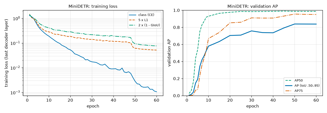
There are four things to read from this figure.
- The stall in the first three epochs. Validation AP is near the floor at 0.0048 → 0.0140 → 0.0405. The loss is falling, 12.6 → 10.1 → 8.8, but AP does not follow, then suddenly starts rising to 0.1456 at epoch 4 and 0.3426 at epoch 6. Early in training the predictions are nearly random, so the matching changes a lot from step to step (the query handling a given object keeps changing), and the cross-attention does not yet know where to look. This experiment did not directly measure how much the matching changes, so this is noted only as a possible explanation.
- AP50 rises fast, AP75 slowly. AP50 is already 0.9294 at epoch 10. At the same point AP75 is 0.6682, rising over dozens of epochs to 0.8523 at epoch 20, 0.9104 at epoch 30 and 0.9549 at epoch 50. As learned in Chapter 3, AP50 counts a hit "once IoU exceeds 0.5," while AP75 requires "exceeding 0.75." The model quickly learns to find objects roughly, but takes a long time to fit the boxes precisely. The left panel tells the same story. The classification loss (blue line) drops steeply, reaching 0.001 by the end, but the two box-loss terms decrease much more slowly and make up nearly all of the loss at the end.
- A step where the learning rate drops. When the learning rate is cut to one tenth after epoch 48, the loss falls like a step (0.9123 at epoch 45 → 0.5119 at epoch 50), and AP rises from 0.7923 to 0.8386. Boxes that wobbled around the ground truth at the large learning rate settle into place at the small one.
- Fluctuation. AP dips slightly from 0.7576 at epoch 30 to 0.7381 at epoch 35 and 0.7358 at epoch 40, then rises again. With a single seed and measurements every 5 epochs, it is hard to read meaning into ups and downs of this size.
It is also worth noting that AP stopped at 0.84. Since AP50 is 0.986, nearly all objects are found. AP is the average over ten IoU thresholds from 0.50 to 0.95 (Chapter 3), so it loses points at strict thresholds such as 0.90 and 0.95. In a 96-pixel image, exceeding such an IoU requires each box edge to be within one or two pixels.
Prediction examples
- Figure: Figure 7-4 Predictions on validation images 0 – 7. White dashed lines are ground truths; green solid lines are predictions with score 0.5 or higher (labels show the class and score). "k pred / m gt" in each title is the number of predictions with score 0.5 or higher and the number of ground truths.
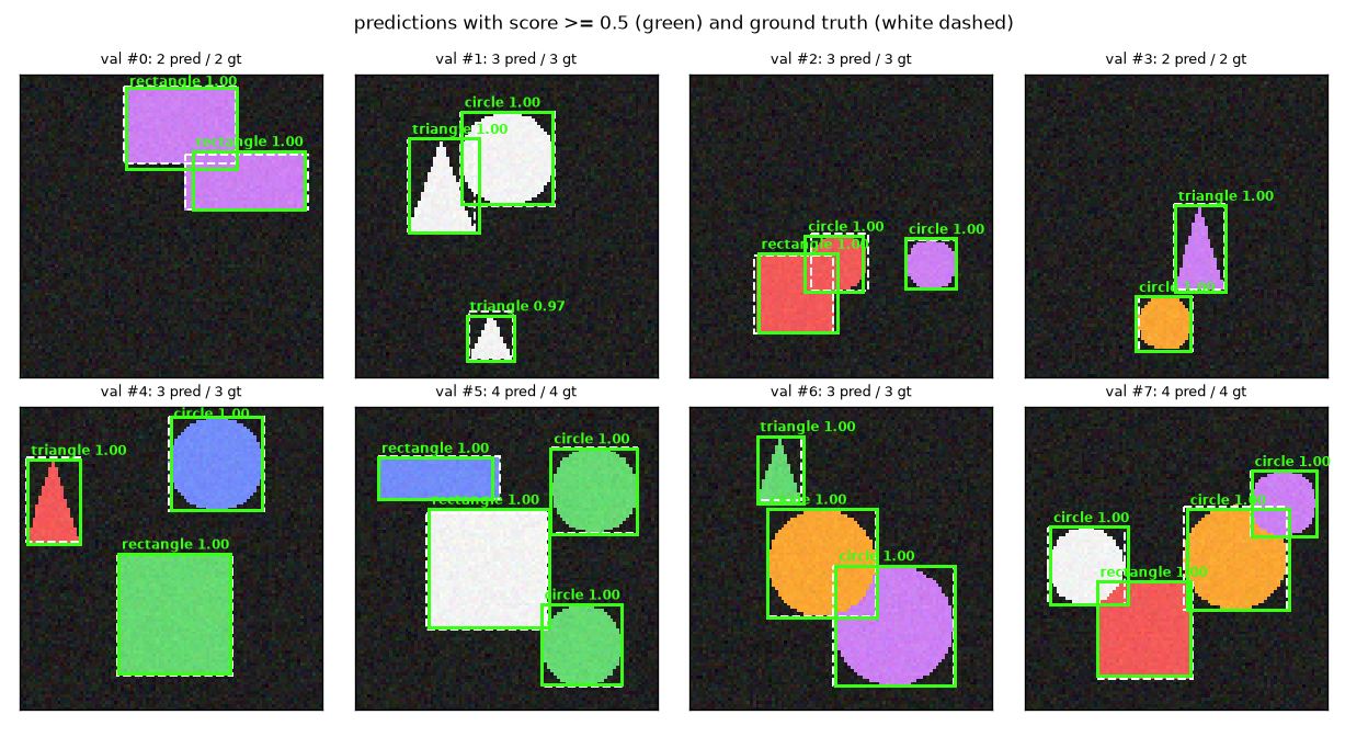
- In all eight images the number of predictions equals the number of ground truths, and the green solid lines nearly coincide with the white dashed lines. Most scores are 1.00; only the small triangle in image 1 is 0.97.
- Even in images where shapes overlap (images 2, 6 and 7), there is one box per object. Despite there being no NMS, nowhere do two green boxes overlap on the same object.
- These eight images are not the whole story, though. Of the 500 validation images, 443 have the same number of predictions with score 0.5 or higher as ground truths, and 57 differ. It is "right most of the time," not "always right."
Query specialization
The object queries are 12 fixed vectors independent of the image. After training, what has each query come to handle? We plot the centers of the boxes produced by each query across all 500 validation images. This is the same kind of figure as Figure 7 of the paper.
- Figure: Figure 7-5 Centers of predicted boxes per query (500 validation images). Each panel is one query, and each point is that query's prediction on one image. Colored points are predictions with score 0.5 or higher: green circles are small boxes (longer side less than 0.28 of the image), orange squares are large wide boxes, and blue triangles are large tall boxes. Pale gray points have score below 0.5 (images where the query answered "no object"). "object in k%" in each title is the fraction of images in which that query produced a score of 0.5 or higher.
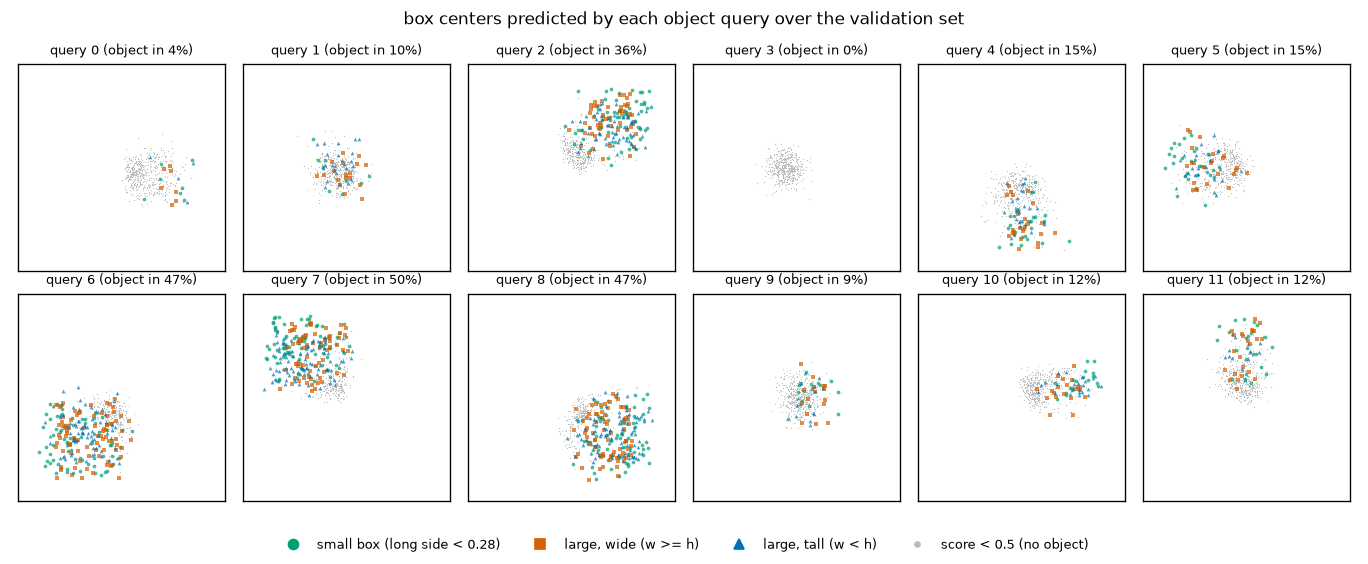
[질의의 전문화] 질의별로: 점수≥0.5 로 '객체가 있다' 고 답한 그림의 비율, 그때 낸 박스의 평균(± 표준편차)
질의 | 쓰인 비율 | 중심 x        중심 y        | 너비          높이
  0  |   0.04    | 0.75 ± 0.07   0.57 ± 0.08  | 0.26 ± 0.08   0.27 ± 0.06
  1  |   0.10    | 0.47 ± 0.07   0.50 ± 0.07  | 0.30 ± 0.07   0.29 ± 0.08
  2  |   0.36    | 0.70 ± 0.09   0.29 ± 0.08  | 0.28 ± 0.08   0.28 ± 0.08
  3  |   0.00    | (거의 쓰이지 않음)
  4  |   0.15    | 0.51 ± 0.06   0.74 ± 0.09  | 0.27 ± 0.08   0.27 ± 0.07
  5  |   0.15    | 0.28 ± 0.09   0.49 ± 0.08  | 0.27 ± 0.08   0.27 ± 0.08
  6  |   0.47    | 0.32 ± 0.10   0.69 ± 0.10  | 0.29 ± 0.08   0.28 ± 0.08
  7  |   0.50    | 0.30 ± 0.10   0.29 ± 0.09  | 0.27 ± 0.08   0.28 ± 0.08
  8  |   0.47    | 0.70 ± 0.09   0.68 ± 0.10  | 0.28 ± 0.08   0.28 ± 0.08
  9  |   0.09    | 0.57 ± 0.06   0.49 ± 0.08  | 0.27 ± 0.09   0.28 ± 0.08
 10  |   0.12    | 0.74 ± 0.08   0.44 ± 0.05  | 0.27 ± 0.08   0.29 ± 0.08
 11  |   0.12    | 0.49 ± 0.06   0.27 ± 0.09  | 0.27 ± 0.08   0.26 ± 0.08
그림마다 점수≥0.5 인 예측 수가 정답 객체 수와 같은 그림: 443 / 500장
- Each query covers a different location. Query 7 covers the top left (center 0.30, 0.29), query 2 the top right (0.70, 0.29), query 6 the bottom left (0.32, 0.69) and query 8 the bottom right (0.70, 0.68) (\(y\) increases downward). These four split the image into four quadrants and are used in 36 – 50% of images, while the queries covering the center and edges (1, 4, 5, 9, 10, 11) are used in 9 – 15% of images. No one told them "you take the top left." In the course of reducing the loss under one-to-one matching, the queries divided the regions among themselves. Training has effectively taken over the role of the hand-crafted anchors.
- No specialization by size is visible. The paper reports that on COCO each slot covers a different region and box size. In this experiment all three colors are mixed in every panel, and the mean widths and heights in the table are nearly the same for every query, at 0.26 – 0.30. Only positional specialization was confirmed. One possible reason is that object sizes in the shape world are not as varied as in COCO, but this was not verified.
- Some queries go unused. Query 3 never exceeded a score of 0.5 in the 500 images (0%), and query 0 only in 4%. With at most 4 objects per image and 12 queries, it is natural for some to be left over. The usage fractions add up to 2.57, nearly equal to the average of 2.53 objects per image.
- The gray points (boxes in images where the query answered ∅) also cluster in one place for each query. Unmatched queries have no box loss, so when there is no object, the box stays near that query's "default position."
Cross-attention maps
We can also see where in the image a query looks when producing its box. For validation image 1 (3 objects), we plotted the last decoder layer's cross-attention weights of the three queries with score 0.5 or higher. One query's weights form a probability distribution (summing to 1) over the 144 image tokens, so they can be drawn as a \(12 \times 12\) map (averaged over the 8 heads).
- Figure: Figure 7-6 Cross-attention on validation image 1. Left: the image and ground-truth boxes. The three panels on the right show the last decoder layer's cross-attention maps of queries 2, 4 and 7 (brighter means larger weight) with each query's predicted box (green). Each panel has its own color scale.
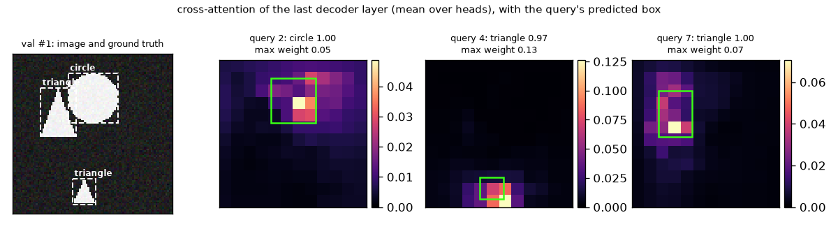
[교차 어텐션] 검증 그림 #1: 점수≥0.5 인 질의 [2, 4, 7]. 지도는 144칸에 걸친 확률 분포(합 1)이고, 칸마다 고르게 보면 1/144 = 0.0069
  질의 2: 가장 큰 가중치 0.049, 상위 5칸의 합 0.171
  질의 4: 가장 큰 가중치 0.126, 상위 5칸의 합 0.406
  질의 7: 가장 큰 가중치 0.071, 상위 5칸의 합 0.210
- Each query looks near its own object. For query 2 the area near the circle at the top is bright, for query 4 the small triangle at the bottom, and for query 7 the triangle at the top left. This agrees with the regions seen in the table above (query 2 top right, query 4 bottom center, query 7 top left).
- Far more concentrated than uniform attention. Uniform attention over 144 cells would give 0.0069 per cell, but the largest weights are 0.049 – 0.126, 7 – 18 times that. The top 5 cells account for 17 – 41% of the weight.
- It does not cover the whole box evenly. The bright cells cluster in a few cells inside and around the box, and for queries 4 and 7 the brightest cell is on the bottom edge of the box. The paper likewise observes that decoder attention is fairly local and mostly looks at object extremities (such as heads or legs), and hypothesizes that since the encoder has already separated the objects, the decoder only needs to read off their boundaries. Our figure is a single image, so all we can say is that "the same kind of pattern is visible."
Per-layer AP and the NMS experiment
Now for the experiment promised in Chapter 3. We apply Chapter 3's nms to the trained DETR's output to see whether it is really unnecessary. Thanks to the auxiliary losses, every decoder layer produces predictions, so for each layer we measure the following.
- AP measured on that layer's predictions, and AP after applying per-class NMS (IoU threshold 0.5)
- The number of predictions with score 0.5 or higher
- The number of pairs among those predictions that overlap each other with IoU above 0.5. The shape world is generated so that IoU between ground truths never exceeds 0.2, so such pairs point at one object twice (duplicate predictions).
def apply_nms(predictions, iou_threshold: float = 0.5):
    """예측 목록에 클래스별 NMS 를 건다 (3장의 nms). DETR 에는 필요 없음을 확인하는 용도."""
    kept = []
    for pred in predictions:
        keep = []
        for cls in pred["labels"].unique():
            index = torch.nonzero(pred["labels"] == cls).flatten()
            chosen = nms(box_cxcywh_to_xyxy(pred["boxes"][index]), pred["scores"][index], iou_threshold)
            keep.append(index[chosen])
        keep = torch.cat(keep) if keep else torch.zeros(0, dtype=torch.long)
        kept.append({k: v[keep] for k, v in pred.items()})
    return kept

def count_duplicates(predictions, score_threshold: float = 0.5, iou_threshold: float = 0.5):
    """점수가 문턱값 이상인 예측끼리 IoU 가 iou_threshold 를 넘게 겹치는 쌍의 수 (클래스 무관).

    도형 세상의 정답끼리는 IoU 가 0.2 를 넘지 않으므로, 이런 쌍은 "한 객체를 두 번 예측한 것" 이다.
    돌려주는 값: (겹치는 쌍의 수, 점수가 문턱값 이상인 예측의 수).
    """
    pairs, confident = 0, 0
    for pred in predictions:
        boxes = box_cxcywh_to_xyxy(pred["boxes"][pred["scores"] >= score_threshold])
        confident += len(boxes)
        if len(boxes) > 1:
            iou, _ = box_iou(boxes, boxes)
            pairs += int((torch.triu(iou, diagonal=1) > iou_threshold).sum())
    return pairs, confident
[디코더 층별 예측과 중복]
디코더 층 | AP     AP50   AP75  | NMS 뒤 AP  AP50  | 점수≥0.5 예측 수 | 그중 IoU>0.5 로 겹치는 쌍
    1     | 0.8067 0.9742 0.9197 | 0.8082  0.9878 |     1367         |    153
    2     | 0.8365 0.9872 0.9536 | 0.8335  0.9893 |     1305         |     55
    3     | 0.8375 0.9863 0.9500 | 0.8359  0.9884 |     1290         |     45
검증 정답 객체 수 1265개. 마지막 층: 점수≥0.5 예측 1290개, 겹치는 쌍 45개, NMS 전후 AP 차이 -0.0016
- Figure: Figure 7-7 AP (left) and AP50 (right) per decoder layer. The blue solid line is without NMS; the orange dotted line is after applying NMS. The vertical axes have a very narrow range (AP 0.805 – 0.84, AP50 0.974 – 0.990). Be careful not to read the gaps between lines as large.
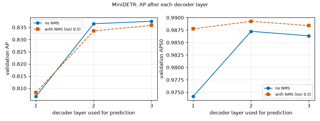
Here is what to read from the table and figure.
- Last layer: NMS brings no gain. Applying NMS lowers AP by 0.0016, from 0.8375 to 0.8359, and raises AP50 by 0.0021, from 0.9863 to 0.9884. In effect there is no change. Compared with Chapter 3's experiment, where applying NMS to predictions with many duplicates raised AP substantially, this means the model's output has almost no duplicates for NMS to profit from removing.
- That does not mean there are zero duplicates. In the last layer there are 1,290 predictions with score 0.5 or higher, 25 more than the 1,265 ground truths, and 45 pairs overlap each other, about 3.6% of the 1,265 objects. What this experiment shows is not "DETR produces no duplicates at all" but "duplicates are rare even without NMS, and applying NMS gains nothing."
- The first layer has many duplicates. The first layer's output has 153 overlapping pairs (about 12% of the objects), and NMS raises AP50 by 0.0136, from 0.9742 to 0.9878. Through the layers, overlapping pairs drop 153 → 55 → 45, and NMS's AP50 gain shrinks +0.0136 → +0.0021 → +0.0021. As the note box above explained, the first layer's queries had no chance to talk to each other after seeing the image. From the second layer on, they coordinate through self-attention and duplicates decrease.
- The effect of the auxiliary losses. The first layer's output alone gives AP 0.8067. Passing through more layers raises it to 0.8365 and 0.8375. "A slightly less accurate but faster model using fewer decoder layers" is actually obtained.
This picture points in the same direction as what the DETR paper reported on COCO (Figure 4 of the paper). According to the paper, NMS improves performance on the first decoder layer's predictions, but the gain shrinks with depth, and in the last layers it wrongly removes true positives and lowers AP slightly. The magnitudes should not be conflated, however. The paper reports an AP difference of 8.2 between the first and last layers of a 6-layer decoder, whereas in this chapter's 3-layer mini model it is 0.03. Also, differences of about ±0.002 in our results (before and after NMS in the second and third layers) were measured with a single seed and may be within chance.
- Why NMS slightly lowers AP
- NMS keeps the higher-scoring one of overlapping predictions. But the higher-scoring one is not necessarily the one with the more accurate box. If the less accurate box survives, it is still correct at the IoU 0.5 criterion (AP50) but wrong at stricter thresholds, so AP50 can go up while AP goes down. This experiment did not count how many such predictions there actually were, so this is noted only as a possible explanation.
The paper's slow convergence and this experiment
DETR is known for being "slow to train." The numbers the paper reported are as follows.
- DETR paper: on COCO (about 118,000 training images), the ablation experiments were trained for 300 epochs (3 days on 16 V100 GPUs), and the main experiments compared against Faster R-CNN were trained for 500 epochs; the 500-epoch schedule gave 1.5 higher AP than the 300-epoch one. The paper itself notes that it "requires extra-long training schedules."
- Deformable DETR paper: points out that DETR needs 500 epochs to converge on COCO, 10 – 20 times slower than Faster R-CNN.
This chapter's experiment does not reproduce that slowness. The mini DETR exceeds AP 0.5 at epoch 9 and reaches 0.84 at epoch 60 (7,500 steps). Since this differs from expectations, it is recorded as is. Points worth considering as to why it might differ are as follows (none were verified with separate experiments).
- Fewer places to look. The cross-attention has only 144 image tokens to scan. In the paper's setting, even at stride 32 a single image yields around a thousand tokens (for example, \(25 \times 38 = 950\) for \(800 \times 1216\) pixels).
- The problem is easy. The background is dark and simple, the shapes are large relative to the image, and there are 3 classes, at most 4 objects and 12 queries.
- An "epoch" is a different size. Our epoch is 125 steps. The paper's 500 epochs are about 920,000 steps at batch size 64 (\(118{,}000 \times 500 / 64\)).
Still, traces of slowness appeared in two places: the stall in the first three epochs (AP below 0.05) and AP75 and AP rising slowly over dozens of epochs even after AP50 had topped out. "Slow" is always relative to something. In Chapter 8, Deformable DETR is trained on the same data with the same training loop and its curve is overlaid on this one. Then we can judge whether this chapter's curve was the slow one.
Limitations of DETR
DETR changed the framework of detection, but as is it was a hard model to use. In its conclusion the paper itself lists "training, optimization and performance on small objects" as new challenges, and the Deformable DETR paper, published the same year, traced their causes to the architecture. In summary there are three.
- Slow convergence. As seen above, 500 epochs on COCO. The Deformable DETR paper's diagnosis is that right after initialization, attention gives nearly equal weight to every cell of the feature map, and it takes long training for those weights to learn to concentrate on the sparse meaningful locations. The post-training cross-attention in this chapter's experiment, concentrated at 7 – 18 times the uniform value (0.0069), is what "after learning" looks like.
- Weak on small objects. In Table 1 of the paper (COCO), DETR and Faster R-CNN-FPN+ have the same AP of 42.0, but on small objects DETR is lower, with APS of 20.5 against Faster R-CNN's 26.6, and on large objects DETR is higher, with APL of 61.1 against 53.4. Finding small objects requires a high-resolution feature map, but DETR uses only a single coarse feature map at stride 32.
- The encoder's quadratic cost. Then why not raise the feature map's resolution? The encoder's self-attention has every token look at every token, so the cost grows with the square of the number of tokens (Chapter 5). The mini model has \(144^2 = 20{,}736\) pairs, but 950 tokens give \(950^2 = 902{,}500\) pairs, and doubling the resolution in both width and height makes 4 times as many tokens and 16 times as many pairs, \(14{,}440{,}000\). The DETR paper likewise notes that in the variant with doubled resolution (DETR-DC5), the cost of encoder self-attention increases 16-fold and the overall computation doubles. It is an architecture in which raising resolution for small objects is hard.
The three limitations share a single root: attention looks at every cell of the image. Because it looks at every cell, it takes a long time to learn where to look, and because it looks at every cell, the cost becomes unmanageable as the cells multiply. Deformable DETR in the next chapter replaces "every cell" with "a few necessary places" and relieves all three at once. The matching and loss built in this chapter carry over almost unchanged.
Summary
- DETR treats detection as set prediction. A fixed number \(N\) of slots (object queries) each produce one (class, box), and the leftover slots answer "no object (∅)." The outputs are
(B, N, K+1)and(B, N, 4). - Predictions and ground truths are unordered sets, so before computing the loss, the one-to-one assignment \(\hat{\sigma}\) with the minimum total cost is found from the cost matrix \(C\) \((N, T)\) (bipartite matching). There are \(N!/(N-T)!\) assignments, too many to try all of them, but the Hungarian algorithm family (
linear_sum_assignment) finds the exact optimum quickly. Greedy assignment may not be optimal. - The matching cost is \(C_{ij} = -\hat{p}_i(c_j) + 5\,\lVert \hat{b}_i - b_j \rVert_1 - 2\,\operatorname{GIoU}(\hat{b}_i, b_j)\). The class term uses probabilities rather than logs to match the scale of the box terms. Matching only decides indices, so it has no gradient.
- The set loss is the cross-entropy over all queries (the ground-truth class if matched, ∅ otherwise, with ∅ weighted 0.1) + the box loss of matched queries (\(5 \cdot \text{L1} + 2 \cdot (1 - \operatorname{GIoU})\), divided by the number of objects in the batch).
- Under one-to-one matching, if two queries point at one object, one of them is necessarily penalized and must predict ∅. Since the queries see each other and coordinate through the decoder's self-attention, duplicate predictions decrease and NMS becomes unnecessary.
- The architecture is CNN backbone → 1×1 convolution → flatten + 2D sinusoidal positional encoding → encoder → decoder (self-attention → cross-attention → FFN) → classification head and box head (sigmoid). The object queries are learned positional embeddings, the decoder input is zeros, and the \(N\) outputs come out in parallel.
- The auxiliary losses apply the same loss with the same heads to the outputs of all decoder layers (rematching per layer). So predictions come out wherever you stop, which is the basis for RF-DETR being able to drop decoder layers at inference.
- In this chapter's experiment, the mini DETR reached AP 0.8375 (AP50 0.9863) at 60 epochs. The queries divided the image into regions by position (no specialization by size was seen), and applying NMS to the last layer's output gave no gain, only lowering AP by 0.0016. Duplicates were not zero but rare (45 overlapping pairs; 153 in the first layer).
- On this small dataset, the slow convergence the paper reported on COCO (500 epochs) was not reproduced. Traces appeared only in the stall in the first three epochs and the slowly rising AP75.
- DETR's limitations are slow convergence, small objects and the encoder's quadratic cost, all stemming from "attention looks at every cell."
We now have a detector in hand: one trained with nothing but matching and a set loss, without anchors or NMS. But its attention looks at every cell of the image, so it takes long to learn, and raising the resolution makes the cost grow quadratically, so it misses small objects. Deformable DETR in Chapter 8 solves this with deformable attention, in which each query looks at only a few places around a reference point. It takes this chapter's HungarianMatcher and SetCriterion as they are, swaps only the classification loss for the focal loss, and overlays its training curve on this chapter's in the same shape world.
Review questions
- 1. Matching by hand — The cost matrix for 3 predictions and 2 ground truths is as follows (rows = predictions 0, 1, 2 / columns = GT 0, 1). \(C = \begin{pmatrix} 1 & 2 \\ 2 & 6 \\ 5 & 4 \end{pmatrix}\) (a) How many assignments are there in total? (b) Compute the total cost of every assignment and find the optimal one. (c) What is the total cost of the greedy assignment that picks in order starting from GT 0?
- (a) \(3!/(3-2)! = 3 \times 2 = 6\).
- (b) Writing assignments as (partner of GT 0, partner of GT 1): \((0,1)\): \(1 + 6 = 7\), \((0,2)\): \(1 + 4 = 5\), \((1,0)\): \(2 + 2 = 4\), \((1,2)\): \(2 + 4 = 6\), \((2,0)\): \(5 + 2 = 7\), \((2,1)\): \(5 + 6 = 11\). The optimum is \((1, 0)\), i.e., GT 0 ↔ prediction 1 and GT 1 ↔ prediction 0, with total cost 4. Prediction 2 learns ∅.
- (c) GT 0 takes the cheapest, prediction 0 (cost 1), and GT 1 chooses prediction 2 from the remaining prediction 1 (6) and prediction 2 (4). The total cost is \(1 + 4 = 5\), 1 more than the optimum. It has the same form as the example in the text: prediction 0 is useful for both ground truths, so it is better to yield it to GT 1.
- 2. Counting — RF-DETR's detection models use 300 queries. How many assignments are possible for an image with 5 objects? At \(10^{9}\) assignments per second, how long would trying them all take?
- \(300 \times 299 \times 298 \times 297 \times 296 = 2{,}349{,}940{,}507{,}200 \approx 2.35 \times 10^{12}\) assignments. \(2.35 \times 10^{12} / 10^{9} \approx 2{,}350\) seconds, about 39 minutes. Matching a single image with only 5 objects at a single step would take that long, so brute-force search is unusable.
- 3. One cell of the matching cost — The predicted box is \((0.50, 0.50, 0.20, 0.20)\), the ground-truth box is \((0.55, 0.50, 0.20, 0.20)\), and the prediction gave the ground-truth class a probability of 0.8. Compute DETR's matching cost (coefficients 1, 5, 2).
- Class term: \(-0.8\). L1: \(|0.50 - 0.55| + 0 + 0 + 0 = 0.05\).
- In corner representation the prediction is \((0.40, 0.40, 0.60, 0.60)\) and the ground truth \((0.45, 0.40, 0.65, 0.60)\). Intersection \((0.60 - 0.45) \times (0.60 - 0.40) = 0.15 \times 0.20 = 0.03\), union \(0.04 + 0.04 - 0.03 = 0.05\), \(\operatorname{IoU} = 0.6\). The enclosing box is \((0.65 - 0.40) \times 0.20 = 0.05\), the same as the union (the box was only shifted sideways, so there is no empty space), so \(\operatorname{GIoU} = 0.6 - 0 = 0.6\).
- \(C = -0.8 + 5 \times 0.05 - 2 \times 0.6 = -0.8 + 0.25 - 1.2 = -1.75\).
- 4. Set loss by hand — One image with 3 queries and 1 ground truth (rectangle). Matching made query 0 the ground truth's partner. Query 0 gave rectangle a probability of 0.5, its L1 distance to the partner is 0.10, and the GIoU is 0.70. Queries 1 and 2 gave ∅ 0.9 and 0.6, respectively. Following this chapter's implementation, compute \(\mathcal{L}_{\text{cls}}\), \(\mathcal{L}_{\text{L1}}\), \(\mathcal{L}_{\operatorname{GIoU}}\) and the total loss. (\(-\log 0.5 = 0.6931\), \(-\log 0.9 = 0.1054\), \(-\log 0.6 = 0.5108\))
- Classification: the weighted sum is \(1 \times 0.6931 + 0.1 \times 0.1054 + 0.1 \times 0.5108 = 0.6931 + 0.0105 + 0.0511 = 0.7547\), and the sum of weights is \(1 + 0.1 + 0.1 = 1.2\). \(\mathcal{L}_{\text{cls}} = 0.7547 / 1.2 = 0.6289\).
- Boxes: there is 1 object, so \(\mathcal{L}_{\text{L1}} = 0.10 / 1 = 0.10\) and \(\mathcal{L}_{\operatorname{GIoU}} = (1 - 0.70) / 1 = 0.30\).
- Total: \(0.6289 + 5 \times 0.10 + 2 \times 0.30 = 0.6289 + 0.5 + 0.6 = 1.7289\). The boxes of queries 1 and 2 were not used anywhere.
- 5. What changes the assignment — Answer for the \(4 \times 3\) cost matrix in the text. (a) Does adding 2 to every cell change the optimal assignment? (b) What about adding 10 to the entire GT 1 column? (c) What about adding 10 to the entire prediction 0 row?
- (a) No. Every assignment uses three cells, so every assignment's total cost increases by the same 6. This is why the paper's \(1 - \operatorname{GIoU}\) and the code's \(-\operatorname{GIoU}\) give the same assignment.
- (b) No. Every assignment uses exactly one cell in the GT 1 column, so all increase by 10.
- (c) Yes. There are more predictions than ground truths, so some assignments do not use prediction 0, and their total cost stays the same. In the table in the text, the best assignment not using prediction 0 is \((1, 3, 2)\) at 0.1237, while every assignment using prediction 0 increases by 10, so the best of them becomes \(-1.9587 + 10 = 8.0413\). The new optimal assignment is \((1, 3, 2)\). This is why only subtracting from columns was said to be safe for a rectangular matrix.
- 6. Duplicate predictions and ∅ — Queries A and B produced nearly the same box on one triangle. A gave triangle 0.95; B gave triangle 0.75 and ∅ 0.20. Matching chose A as the partner. (a) What is B's target class, and what does B add to the numerator of the classification loss? (\(-\log 0.2 = 1.609\)) (b) What loss does B's box receive? (c) What would become difficult without self-attention among the queries?
- (a) The target is ∅. \(0.1 \times (-\log 0.2) = 0.1 \times 1.609 = 0.161\). Even though it got the triangle right, it is penalized with "you should have answered ∅."
- (b) None. The box loss applies only to matched queries. Only B's score is penalized.
- (c) B would have no way of knowing that "A has taken this triangle." If each query answered separately by looking only at the image, there would be no way to decide which of two queries that both see the same object clearly should back off. In the experiment in the text, the first decoder layer's output, where the queries had no chance to talk to each other, had the most overlapping pairs, at 153.
- 7. Reading the loss in the log — The last line of the training log is
손실 0.4232 (ce 0.0011 bbox 0.0104 giou 0.0383). (a) Compute the weighted sum for the last decoder layer from the three values in parentheses. (b) How many times larger is the "loss" of 0.4232? Why? - (a) \(1 \times 0.0011 + 5 \times 0.0104 + 2 \times 0.0383 = 0.0011 + 0.0520 + 0.0766 = 0.1297\).
- (b) \(0.4232 / 0.1297 \approx 3.26\) times. The "loss" is the sum of the losses of all three decoder layers (the main loss + 2 auxiliary losses). It is 3.26 rather than exactly 3 because the earlier layers' losses are slightly larger than the last layer's (the other two layers sum to \(0.4232 - 0.1297 = 0.2935\), an average of 0.147 per layer). This agrees with predictions improving through the layers.
- 8. Shapes and cost — Feed one \(800 \times 1216\) pixel image into the DETR paper's setting (\(D = 256\), \(N = 100\), stride 32). (a) How many image tokens are there? (b) How many entries do the weight tables of encoder self-attention and decoder cross-attention have (per head)? (c) If the stride is changed to 16, by what factor does each of the two values in (b) grow?
- (a) \(800 / 32 = 25\) and \(1216 / 32 = 38\), so \(25 \times 38 = 950\) tokens.
- (b) Encoder self-attention is tokens × tokens, so \(950 \times 950 = 902{,}500\) entries; decoder cross-attention is queries × tokens, so \(100 \times 950 = 95{,}000\) entries.
- (c) The tokens become \(50 \times 76 = 3{,}800\), 4 times as many. Encoder self-attention grows \(4^2 = 16\) times (\(14{,}440{,}000\) entries) and decoder cross-attention 4 times (\(380{,}000\) entries). It is the encoder, not the decoder, that gets heavier. This matches the paper's note that in DETR-DC5, with doubled resolution, the cost of encoder self-attention increased 16-fold.
See also
Favorite site
- 07. DETR: Detection as Set Prediction
- code/ch07_detr.py
- End-to-End Object Detection with Transformers (DETR, arXiv:2005.12872)
- Deformable DETR: Deformable Transformers for End-to-End Object Detection (arXiv:2010.04159)
- RF-DETR: Neural Architecture Search for Real-Time Detection Transformers (arXiv:2511.09554)