RF-DETR:Tutorial:06-ViT-DINOv2
lastmod 2026-11-18created 2026-11-184 edits
Vision Transformer and DINOv2 is chapter 6 of the RF-DETR tutorial. To feed images into the Transformer encoder built in chapter 5, it builds a Vision Transformer (ViT), which turns an image into a sequence of small pieces (patches), and then covers DINO, a way to train that ViT without a single label, and its successor DINOv2. A ViT pretrained with DINOv2 is exactly the backbone of RF-DETR. The next chapter builds DETR, the first detector to tackle detection head-on with a Transformer.
Topics: why patch embedding is the same computation as a single convolution; the token count \(N = (H/p)(W/p)\) and a by-hand, part-by-part count of the roughly 22 million parameters in ViT-S; compute versus resolution and patch size, and position embedding interpolation (the basis of the NAS knobs in chapter 12); why ViT needs large datasets, and pretraining versus fine-tuning; DINO self-distillation (the student and the EMA teacher, temperature, cross-entropy, collapse and the centering and sharpening that prevent it); DINOv2 and register tokens; why RF-DETR chose this backbone; and PyTorch implementations of MiniViT and a mini DINO, with their results.
- Source text: 06. Vision Transformer and DINOv2
- Hands-on code:
code/ch06_vit.py(checking patch embedding and parameter counts, supervised MiniViT training, changing resolution, position embeddings, mini DINO, collapse experiments, linear classifier, CLS attention). All experiments take about 10 min 30 s on an 8 GB laptop GPU;--quickis a reduced version for catching errors. Patch features from the real DINOv2 are shown bycode/ch06_dinov2_features.py. Reading time for the source text is about 90 minutes; difficulty ★★★☆☆. - Previous: 05. Attention and Transformer / Next: 07. DETR: detection as set prediction
The detector's eyes: the backbone
Recall the big picture of RF-DETR from chapter 1. When an image comes in, the backbone first turns it into a feature map, the projector refines that map, and the decoder looks into the feature map to output boxes and classes. However smart the decoder is, it cannot find anything if the backbone's features carry no information that "something is here". A detector's accuracy depends heavily on how good the backbone's features are.
In RF-DETR, the backbone sits here (figure 6-1 in the source text). An image (B, 3, H, W) passes in turn through the backbone (a ViT pretrained with DINOv2, this chapter) → the projector (chapters 9 and 10) → the decoder (chapters 7–10) and becomes boxes and classes. The backbone turns the image into "a feature vector per patch", and every later component sees only these features. This chapter covers just the backbone box.
In one line, RF-DETR's backbone is "a ViT pretrained with DINOv2". That phrase contains three questions, and this chapter takes them in order.
- What is a ViT? How does it turn an image into a token sequence and feed it to a Transformer? How big is it, and how slow?
- Why is pretraining needed, and how is it done without labels? DINO's self-distillation, and DINOv2.
- Why did RF-DETR choose it, and how does it adapt it?
Turning an image into a token sequence
The Transformer encoder of chapter 5 takes a tensor of shape (B, T, D), that is, "a sequence of \(T\) vectors (tokens) of length \(D\)". For a sentence this is natural, since each word is a token. What about an image? If each pixel is a token, even a 96×96 image has 9,216 tokens. Self-attention computes over every pair of tokens, giving \(9216^2 \approx 8{,}500\) million (85 million) pairs. That is far too many.
The Vision Transformer (ViT) of Dosovitskiy et al. (2020) gave the simplest answer: cut the image into a grid like a checkerboard and treat each square as one token. That is what the paper title "An Image is Worth 16x16 Words" means: a 16×16-pixel piece is one word. After that, it uses the standard Transformer encoder almost unchanged.
Cutting into patches
The image is cut into non-overlapping square pieces with sides of \(p\) pixels. Each piece is called a patch, and \(p\) is the patch size. With image height \(H\) and width \(W\) (in this chapter \(H\) and \(W\) are always the image's size in pixels), there are \(H/p\) rows and \(W/p\) columns, so the number of patches \(N\) is:
\(N = \frac{H}{p}\cdot\frac{W}{p} = \frac{HW}{p^2}\)
\(N\) is the number of tokens the Transformer processes (the single CLS token added shortly is counted separately). \(H\) and \(W\) must be divisible by \(p\). The "/16" or "/14" in a model name is the patch size: ViT-S/14 means "a Small ViT with patch size 14".
- Counting tokens by hand
- \(\text{Shape World: } H = W = 96,\ p = 8 \;\Rightarrow\; \frac{96}{8} = 12,\quad N = 12 \times 12 = 144\)
- The setting used by this chapter's exercises: 12 patches per side, 144 in total.
- DINOv2 uses patch size 14 and does most of its pretraining at 224×224.
- At the end of pretraining, DINOv2 briefly raises the resolution to 518×518 (covered later). This is why the position embeddings in the released DINOv2 weights form a 37×37 grid.
- RF-DETR nano uses resolution 384 and patch size 16 (table 7 of the paper). 576 tokens pass through the backbone.
- Figure: Figure 6-2 Left: a 96×96 Shape World image with patch boundaries drawn. Right: the 144 cut-out 8×8 patches. Tokens are numbered in reading order (top left → right → next row).
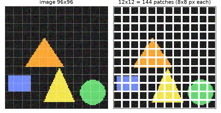
There are two things to read from figure 6-2. First, most patches are background, and a shape spans several patches. From one patch alone it is hard to tell whether it is part of a circle or the hypotenuse of a triangle. That is why self-attention, which lets patches exchange information, is needed. Second, the moment the patches are laid out in a single row, "which patch is next to or below which" is lost. Tokens 12 and 13 are neighbors in the sequence, but in the image they are the right end of one row and the left end of the next. This information is restored later with position embeddings.
Patch embedding: flatten and project linearly
A patch is \(p \times p\) pixels with \(C = 3\) color channels, so it holds \(C p^2\) numbers. Flattened, it becomes a vector of length \(Cp^2\); in Shape World, \(3 \times 8 \times 8 = 192\). Because the Transformer takes tokens of length \(D\), a single learned linear layer is applied to this vector to map it to length \(D\). Let \(x_n \in \mathbb{R}^{Cp^2}\) be the flattened \(n\)-th patch, \(E \in \mathbb{R}^{D \times Cp^2}\) the linear layer's weights and \(b \in \mathbb{R}^{D}\) its bias. Then
\(e_n = E\,x_n + b \;\in \mathbb{R}^{D}, \qquad n = 1, \dots, N\)
This \(e_n\) is called the patch embedding. Every patch uses the same \(E\) and \(b\). Each row of \(E\) (length \(Cp^2\)) is a template saying "respond strongly to patches with this pattern", and there are \(D\) such templates.
But "applying the same weights identically at many places in an image" is the definition of convolution seen in chapter 4. In fact, patch embedding is exactly the same computation as a single convolution whose kernel size and stride are both \(p\). Chapter 4 only checked this numerically at the end; here it is worked out with equations.
- Patch embedding = convolution with kernel and stride p
- \(y[k, i, j] = \sum_{c=1}^{C}\sum_{u=0}^{p-1}\sum_{v=0}^{p-1} K[k, c, u, v]\; I[c,\; s\,i + u,\; s\,j + v] + b[k]\)
- The definition of convolution. \(I\) is the input image, \(K\) a kernel of shape \((D, C, p, p)\), \(s\) the stride (the step by which the window moves), and \(y[k, i, j]\) the output at channel \(k\), row \(i\), column \(j\).
- The stride is set equal to the kernel size. The window jumps \(p\) cells at a time, so windows do not overlap, and the \((i, j)\)-th window covers rows \(pi \dots pi + p - 1\) and columns \(pj \dots pj + p - 1\). This is exactly the same region as the \((i, j)\)-th patch.
- \(x_n\) is the \(n = i \cdot (W/p) + j\)-th patch flattened in (channel, row, column) order. The kernel \(K\) is also flattened in the same order for each channel \(k\) and used as the \(k\)-th row of the matrix \(E\). \((c, u, v)\) denotes a single position index within the flattened vector.
- The triple sum is the dot product of the vector \(x_n\) with the \(k\)-th row of \(E\). The length-\(D\) vector at cell \((i, j)\) of the convolution output is the \(n\)-th patch embedding. The two computations perform the same additions and multiplications, just in a different order.
So the implementation is one line of convolution. Flattening the grid of the output (B, D, H/p, W/p) into (B, N, D) gives the token sequence. The patchify below implements "cut into patches and flatten" literally, and check_patch_embed checks that the two approaches give the same output.
def patchify(images: torch.Tensor, patch_size: int) -> torch.Tensor:
    """그림을 패치로 잘라, 패치 하나하나를 한 줄 벡터로 편다.

    images: (B, C, H, W)  →  돌려주는 값: (B, N, C·p·p),  N = (H/p)·(W/p)
    패치 순서는 글 읽는 순서(왼쪽 위에서 오른쪽으로, 다음 줄로)이고,
    한 패치 안의 값은 (채널, 행, 열) 순서로 편다 — 합성곱 가중치 (D, C, p, p) 를 펼 때와 같은 순서여야 한다.
    """
    B, C, H, W = images.shape
    p = patch_size
    gh, gw = H // p, W // p  # 세로 · 가로 패치 수
    x = images.reshape(B, C, gh, p, gw, p)  # 높이를 (패치 줄, 패치 안 행), 너비를 (패치 칸, 패치 안 열)로 쪼갠다
    x = x.permute(0, 2, 4, 1, 3, 5)  # (B, gh, gw, C, p, p): 패치 위치를 앞으로
    return x.reshape(B, gh * gw, C * p * p)
class PatchEmbed(nn.Module):
    """패치 임베딩: 그림 (B, 3, H, W) → 토큰 열 (B, N, D).

    커널 크기 = 스트라이드 = p 인 합성곱 하나다. 창이 겹치지 않고 p 칸씩 건너뛰므로
    "패치마다 같은 선형 층을 한 번씩 적용" 하는 것과 같은 계산이 된다.
    """

    def __init__(self, patch_size: int, dim: int, in_channels: int = 3):
        super().__init__()
        self.patch_size = patch_size
        self.proj = nn.Conv2d(in_channels, dim, kernel_size=patch_size, stride=patch_size)

    def forward(self, images: torch.Tensor) -> torch.Tensor:
        x = self.proj(images)  # (B, D, H/p, W/p): 격자 한 칸이 패치 하나
        return x.flatten(2).transpose(1, 2)  # (B, D, N) → (B, N, D)

def check_patch_embed(log=print):
    """합성곱 방식과 '펴서 선형 투영' 방식이 같은 값을 내는지 확인한다."""
    torch.manual_seed(0)
    embed = PatchEmbed(patch_size=8, dim=96)
    images = torch.rand(2, 3, 96, 96)
    by_conv = embed(images)  # (2, 144, 96)
    weight = embed.proj.weight.reshape(96, -1)  # (D, C, p, p) → (D, C·p·p) = (96, 192)
    by_linear = patchify(images, 8) @ weight.T + embed.proj.bias  # (2, 144, 192) @ (192, 96) → (2, 144, 96)
    diff = (by_conv - by_linear).abs().max().item()
    log(f"[check] 패치 임베딩: 합성곱 {tuple(by_conv.shape)} vs 펴서 선형 투영 {tuple(by_linear.shape)}, 최대 차이 {diff:.2e}")
    assert diff < 1e-5
The \(10^{-6}\) difference is 32-bit floating-point rounding error (from the different order of additions). The two approaches are the same computation.
- Note · patch embedding is "a single, very coarse convolution layer"
- An ordinary convolutional neural network stacks many layers of small kernels such as 3×3 with stride 1–2, reducing resolution gradually. ViT reduces it by a factor of \(p\) all at once in the first layer and never changes the resolution after that. Because one cell of the backbone's output feature map corresponds to \(p \times p\) pixels of the original image, it is called a "stride-\(p\) feature map" or "1/\(p\) resolution". For a 384×384 image, RF-DETR nano's backbone output is a 24×24 grid.
The CLS token and position embeddings
Two more things are added to the \(N\) patch embeddings before they enter the Transformer.
① The CLS token. When a single answer for the whole image is needed, as in image classification, one must decide which of the \(N\) patch outputs to use as the answer. Following the language model BERT, ViT inserts one learned vector \(x_{\text{cls}} \in \mathbb{R}^D\) that belongs to no patch at the front of the sequence. This is the CLS token (class token, [CLS]). It gathers information from all patches through self-attention, and its output at the last layer is used as a summary of the whole image. The token count becomes \(N + 1\).
② Position embeddings. As seen in chapter 5, self-attention does not know the order of tokens. Shuffle the input tokens and the output just comes out shuffled the same way. So "this token came from this part of the image" has to be written directly into the token. The original Transformer in chapter 5 added a fixed positional encoding built from sines and cosines. ViT instead keeps one learned vector per position and adds it. This is the position embedding; with one length-\(D\) vector for each of the \(N + 1\) positions, it is a parameter \(E_{\text{pos}}\) of shape \((N + 1) \times D\).
\(X_0 = \big[\,x_{\text{cls}};\; e_1;\; e_2;\; \dots;\; e_N\,\big] + E_{\text{pos}}, \qquad X_0 \in \mathbb{R}^{(N+1) \times D}\)
\([\,\cdot\,;\,\cdot\,]\) means stacking vectors as rows, and \(X_0\) is the token sequence entering the first block. Position embeddings start as random values and know nothing of 2D structure such as "positions 12 and 13 are far apart in the image". They must figure it out themselves during training (figure 6-6 later checks whether they really do).
- Caution · the size of the position embedding is tied to the resolution
- A convolution kernel can be reused as is when the image grows, but the position embedding is a table with a fixed number of positions, \(N + 1\). Feed a 128×128 image (257 positions) into a model trained at 96×96 (145 positions), and the table runs short. This problem and its solution (interpolation) are covered later in "Changing resolution and patch size". It is a hurdle RF-DETR must clear to use resolution as a knob.
Stacking encoder blocks
Now \(X_0\) passes through \(L\) Transformer encoder blocks from chapter 5 in turn. A block has two parts, multi-head self-attention (tokens exchange information) and an MLP (each token is processed separately), with layer normalization before each part and a residual connection around each part. Equations (2)–(4) of the ViT paper, in this chapter's notation, are as follows (\(\ell = 1, \dots, L\)).
\(\begin{aligned} X'_\ell &= X_{\ell-1} + \mathrm{MSA}\big(\mathrm{LN}(X_{\ell-1})\big) \\ X_\ell &= X'_\ell + \mathrm{MLP}\big(\mathrm{LN}(X'_\ell)\big) \\ Y &= \mathrm{LN}(X_L) \end{aligned}\)
- \(\mathrm{MSA}\) is multi-head self-attention and \(\mathrm{LN}\) is layer normalization.
- \(\mathrm{MLP}\) is two linear layers with a GELU activation function between them. It is the very component called the FFN in chapter 5; the ViT paper calls it the MLP. The hidden dimension in the middle is usually \(4D\), and this 4 is called the MLP ratio.
- Layer normalization sits before attention and the MLP, and the residual addition is outside the normalization. Of the two arrangements seen in chapter 5 (post-norm and pre-norm), this is pre-norm. Because the input is added all the way to the output without passing through normalization, training stays stable even with deep stacks.
- One more layer normalization follows the last block. The first row of the output \(Y \in \mathbb{R}^{(N+1)\times D}\) is the CLS output, and the remaining \(N\) rows are the patch features.
In image classification, a single linear layer (the classification head) on the CLS output produces class scores. In detection, the \(N\) rows of patch features are the stars instead. Folded back into an \((H/p) \times (W/p)\) grid, they form a feature map with \(D\) channels, and the decoder finds objects in this feature map.
Following the tensor shapes
In this chapter's MiniViT (96×96, patch 8, \(D = 96\), 4 layers), tensor shapes change at the following points (figure 6-3 in the source text).
- Image
(B, 3, 96, 96)→ patch embedding (Conv 8×8, stride 8) →(B, 144, 96) - Prepend the CLS token (one at the front) →
(B, 145, 96) - Add position embeddings (parameter
(1, 145, 96)) →(B, 145, 96) - Pre-norm block × 4 (4 heads, MLP hidden 384): x + self-attention(LN(x)) → x + MLP(LN(x)). The shape stays
(B, 145, 96) - After the final layer normalization, the CLS output
[:, 0]is(B, 96), a summary of the whole image, and the patch features[:, 1:]are(B, 144, 96), which become a 12×12 feature map.
Only the first two steps change the shape; the blocks keep (B, 145, 96) throughout. Classification attaches a head to the CLS output, and detection uses the patch features.
The code follows this figure exactly. SelfAttention and Block compute the same thing as in chapter 5 (they are implemented by hand so the attention maps can be extracted; whether the values match PyTorch's built-in nn.MultiheadAttention is checked at run time), and MiniViT ties everything together. The position embedding interpolation inside embed is explained shortly.
class SelfAttention(nn.Module):
    """다중 머리 자기 어텐션 (5장). 어텐션 가중치를 꺼내 볼 수 있게 직접 구현한다.

    x: (B, T, D) → (B, T, D).  T 는 토큰 수(CLS 1개 + 패치 N개), 머리 수 h, 머리 하나의 차원 D/h.
    """

    def __init__(self, dim: int, heads: int):
        super().__init__()
        assert dim % heads == 0
        self.heads = heads
        self.qkv = nn.Linear(dim, dim * 3)  # 질의 · 열쇠 · 값을 한 번에 만든다
        self.proj = nn.Linear(dim, dim)  # 머리들을 다시 합친 뒤의 출력 투영

    def forward(self, x: torch.Tensor, return_attention: bool = False):
        B, T, D = x.shape
        qkv = self.qkv(x).reshape(B, T, 3, self.heads, D // self.heads).permute(2, 0, 3, 1, 4)
        q, k, v = qkv[0], qkv[1], qkv[2]  # 각각 (B, h, T, D/h)
        scores = q @ k.transpose(-2, -1) / math.sqrt(D // self.heads)  # (B, h, T, T)
        attention = scores.softmax(dim=-1)  # 행마다 합이 1: 토큰 i 가 토큰 j 를 보는 비율
        out = (attention @ v).transpose(1, 2).reshape(B, T, D)  # (B, h, T, D/h) → (B, T, D)
        out = self.proj(out)
        return (out, attention) if return_attention else out

class Block(nn.Module):
    """pre-norm Transformer 인코더 블록: x + Attn(LN(x)), 그다음 x + MLP(LN(x))."""

    def __init__(self, dim: int, heads: int, mlp_ratio: int = 4):
        super().__init__()
        self.norm1 = nn.LayerNorm(dim)
        self.attn = SelfAttention(dim, heads)
        self.norm2 = nn.LayerNorm(dim)
        self.mlp = nn.Sequential(nn.Linear(dim, dim * mlp_ratio), nn.GELU(), nn.Linear(dim * mlp_ratio, dim))

    def forward(self, x: torch.Tensor) -> torch.Tensor:
        x = x + self.attn(self.norm1(x))  # 층 정규화를 먼저(pre-norm), 잔차 연결은 정규화 밖에서
        return x + self.mlp(self.norm2(x))
class MiniViT(nn.Module):
    """작은 Vision Transformer.

    그림 (B, 3, H, W)
      → 패치 임베딩 (B, N, D)
      → 맨 앞에 CLS 토큰을 붙여 (B, 1 + N, D)
      → 위치 임베딩을 더함
      → pre-norm 블록 L 개
      → 마지막 층 정규화 → (B, 1 + N, D).   [:, 0] 이 CLS(그림 전체의 요약), [:, 1:] 이 패치 특징.
    num_outputs > 0 이면 CLS 위에 선형 분류 머리를 하나 단다.
    """

    def __init__(self, image_size: int = 96, patch_size: int = 8, dim: int = 96, depth: int = 4, heads: int = 4,
                 mlp_ratio: int = 4, num_outputs: int = 0):
        super().__init__()
        self.patch_size = patch_size
        self.grid = image_size // patch_size  # 학습 해상도에서 한 변의 패치 수 (96 / 8 = 12)
        self.dim = dim
        self.patch_embed = PatchEmbed(patch_size, dim)
        self.cls_token = nn.Parameter(torch.zeros(1, 1, dim))
        self.pos_embed = nn.Parameter(torch.zeros(1, 1 + self.grid**2, dim))  # CLS 자리 1개 + 패치 자리 N개
        self.blocks = nn.ModuleList([Block(dim, heads, mlp_ratio) for _ in range(depth)])
        self.norm = nn.LayerNorm(dim)
        self.head = nn.Linear(dim, num_outputs) if num_outputs > 0 else None
        nn.init.trunc_normal_(self.cls_token, std=0.02)
        nn.init.trunc_normal_(self.pos_embed, std=0.02)

    def embed(self, images: torch.Tensor, interpolate: bool = True) -> torch.Tensor:
        """그림 → 위치 임베딩까지 더한 토큰 열 (B, 1 + N, D)."""
        B, _, H, W = images.shape
        assert H == W and H % self.patch_size == 0, "정사각형이고 패치 크기로 나누어떨어지는 그림만 받는다"
        x = self.patch_embed(images)  # (B, N, D)
        x = torch.cat([self.cls_token.expand(B, -1, -1), x], dim=1)  # (B, 1 + N, D)
        pos = self.pos_embed
        new_grid = H // self.patch_size
        if interpolate and new_grid != self.grid:
            # CLS 자리의 위치 임베딩은 그대로 두고, 패치 자리의 것만 2차원 격자로 보간한다
            patch_pos = interpolate_pos_embed(pos[:, 1:], self.grid, new_grid)
            pos = torch.cat([pos[:, :1], patch_pos], dim=1)
        return x + pos  # 보간을 끄고 격자 크기가 다르면 여기서 모양이 맞지 않아 오류가 난다

    def forward_tokens(self, images: torch.Tensor, interpolate: bool = True) -> torch.Tensor:
        x = self.embed(images, interpolate)
        for block in self.blocks:
            x = block(x)
        return self.norm(x)  # (B, 1 + N, D)

    def forward(self, images: torch.Tensor, interpolate: bool = True) -> torch.Tensor:
        cls = self.forward_tokens(images, interpolate)[:, 0]  # (B, D)
        return self.head(cls) if self.head is not None else cls

    @torch.no_grad()
    def last_attention(self, images: torch.Tensor) -> torch.Tensor:
        """마지막 블록에서 CLS 토큰이 각 패치를 보는 비율. (B, h, grid, grid)"""
        x = self.embed(images)
        for block in self.blocks[:-1]:
            x = block(x)
        last = self.blocks[-1]
        _, attention = last.attn(last.norm1(x), return_attention=True)  # (B, h, 1 + N, 1 + N)
        g = images.shape[-1] // self.patch_size
        return attention[:, :, 0, 1:].reshape(len(images), -1, g, g)  # 0번 행(CLS)의 1번 열부터(패치들)
Counting the size of a ViT
You often see the claim that "ViT-S has about 22 million parameters". Let us count where that number comes from, part by part. It builds intuition for model size and shows where the weight is. There are only two counting rules.
- Linear layer \(\text{Linear}(a \to b)\): \(a \times b\) weights + \(b\) biases = \(ab + b\)
- Layer normalization \(\text{LayerNorm}(D)\): \(D\) scales + \(D\) shifts = \(2D\)
Parameter count per component
We count ViT-S/16 configured for 224×224 images (the standard setting for ImageNet classification): \(D = 384\), \(L = 12\) blocks, 6 heads, MLP ratio 4 (hidden dimension \(4D = 1536\)), patch size \(p = 16\), token count \(N = (224/16)^2 = 196\), and 1,000 classes.
- Parameter count of ViT-S/16
- \(\text{Patch embedding: } \underbrace{3 \cdot 16 \cdot 16}_{768} \cdot 384 + 384 = 294{,}912 + 384 = 295{,}296\)
- A linear layer mapping the flattened patch length \(Cp^2 = 768\) to \(D = 384\) (= a convolution kernel \((384, 3, 16, 16)\) plus bias).
- The CLS token is one vector of length \(D\); the position embedding is one vector of length \(D\) for each of the \(N + 1 = 197\) positions.
- \(\text{Linear}(384 \to 3 \cdot 384)\), which merges the three linear layers producing queries, keys and values, and \(\text{Linear}(384 \to 384)\) after the heads' outputs are combined. The head count 6 appears nowhere. Heads are just a way of splitting the same matrix's output into 6 parts, so they do not change the parameter count.
- \(\text{Linear}(384 \to 1536)\) and \(\text{Linear}(1536 \to 384)\). Twice the attention. Two-thirds of a ViT's parameters are in the MLPs.
- Each block has two layer normalizations (before attention and before the MLP).
- All blocks have the same structure.
- The size of the backbone alone, excluding the classification head: about 21.7 million. This is the value that table 1 of the DINO paper lists as "21M" for ViT-S/16 (that table counts without the head).
- Including a 1,000-class classification head gives about 22.05 million, the commonly quoted "about 22 million". The 12 blocks account for 96.6% of the total.
The same count is turned into a function and compared with parameters() counted on a real model built with the same settings.
def vit_param_count(image_size: int, patch_size: int, dim: int, depth: int, mlp_ratio: int = 4, num_classes: int = 0,
                    in_channels: int = 3) -> dict:
    """ViT 의 매개변수 수를 부품별 공식으로 센다 (가중치 + 편향).

    선형 층 Linear(a, b) 는 a·b + b 개, 층 정규화 LayerNorm(d) 는 2d 개(배율 γ 와 이동 β)이다.
    머리 수는 매개변수 수에 영향을 주지 않는다 (같은 qkv 행렬을 머리 수만큼 나눠 쓸 뿐이다).
    """
    n_patches = (image_size // patch_size) ** 2
    hidden = dim * mlp_ratio
    counts = {
        "patch_embed": in_channels * patch_size * patch_size * dim + dim,
        "cls_token": dim,
        "pos_embed": (1 + n_patches) * dim,
        "block.norm x2": 2 * (2 * dim),
        "block.attn.qkv": dim * 3 * dim + 3 * dim,
        "block.attn.proj": dim * dim + dim,
        "block.mlp.fc1": dim * hidden + hidden,
        "block.mlp.fc2": hidden * dim + dim,
        "final_norm": 2 * dim,
        "head": (dim * num_classes + num_classes) if num_classes else 0,
    }
    counts["block"] = sum(v for k, v in counts.items() if k.startswith("block."))
    counts["total"] = (counts["patch_embed"] + counts["cls_token"] + counts["pos_embed"] + depth * counts["block"]
                       + counts["final_norm"] + counts["head"])
    return counts
[count] ViT-S/16: 패치 임베딩 295,296 + CLS 384 + 위치 임베딩 75,648 + 블록 12 × 1,774,464 + 마지막 LN 768 + 분류 머리 385,000 = 22,050,664
        블록 하나: LN 2개 1,536 + qkv 443,520 + proj 147,840 + MLP 591,360 + 590,208
        실제로 만든 모델 22,050,664개 → 일치 (분류 머리 빼면 21,665,664)
[count] ViT-B/16: 패치 임베딩 590,592 + CLS 768 + 위치 임베딩 151,296 + 블록 12 × 7,087,872 + 마지막 LN 1,536 + 분류 머리 769,000 = 86,567,656
        블록 하나: LN 2개 3,072 + qkv 1,771,776 + proj 590,592 + MLP 2,362,368 + 2,360,064
        실제로 만든 모델 86,567,656개 → 일치 (분류 머리 빼면 85,798,656)
| Model | Layers \(L\) | Dimension \(D\) | Heads | MLP hidden | One block | Total (with classification head) | Figure given in the paper |
| ViT-S/16 | 12 | 384 | 6 | 1536 | 1,774,464 | 22,050,664 | 21M (DINO table 1, without head) |
| ViT-B/16 | 12 | 768 | 12 | 3072 | 7,087,872 | 86,567,656 | 86M (ViT table 1) |
ViT-B only doubles the dimension of ViT-S, yet it has almost exactly 4 times the parameters. That is because the heavy parts of a block are all matrices proportional to \(D \times D\) (\(1{,}774{,}464 \times 4 = 7{,}097{,}856 \approx 7{,}087{,}872\); it falls slightly short because terms proportional to \(D\), such as biases and layer normalization, only double). Table 1 of the ViT paper lists only Base (86M), Large (24 layers, \(D = 1024\), 307M) and Huge (32 layers, \(D = 1280\), 632M); Small is a later variant. The DINO paper, saying it follows DeiT's implementation, gives ViT-S as 12 blocks, \(D = 384\) and 6 heads.
Sizes used by DINOv2
The DINOv2 paper (appendix table 17) lists four sizes, all with patch size 14.
| Model | Dimension | Heads | Blocks | MLP type | How it was made |
| ViT-S/14 | 384 | 6 | 12 | MLP | Distilled from ViT-g |
| ViT-B/14 | 768 | 12 | 18 (paper table) / 12 (released config) | MLP | Distilled from ViT-g |
| ViT-L/14 | 1024 | 16 | 24 | MLP (distilled) | Distilled from ViT-g |
| ViT-g/14 | 1536 | 24 | 40 | SwiGLU | Trained from scratch |
- Table 17 of the paper gives 18 blocks for ViT-B/14, but the released config files (including
dinov2_base.jsonin the RF-DETR repository) havenum_hidden_layers: 12. This tutorial follows the released config's 12. - RF-DETR uses only the two smallest of these. Detection N, S, M and L use ViT-S; XL, 2XL and Max use ViT-B (table 7 of the paper).
The released DINOv2 ViT-S/14 weights have exactly 22,056,576 parameters (the value counted by actually downloading them in this chapter's optional exercise). The same counting explains why this differs slightly from the 21,665,664 counted above for the ViT-S/16 backbone.
- Where DINOv2 ViT-S/14's 22,056,576 comes from
- \(\text{Patch embedding: } 3 \cdot 14 \cdot 14 \cdot 384 + 384 = 225{,}792 + 384 = 226{,}176\)
- The patch shrank from 16 to 14, so the kernel is smaller (\(768 \to 588\)).
- The table is sized for the 37×37 grid at 518×518 resolution, so it is much larger than the 197-position one.
- DINOv2's blocks each have one extra learned per-channel scale (LayerScale) multiplied onto the attention and MLP outputs: \(2D\) per block.
- The mask token is the vector placed at masked patch positions during pretraining (the iBOT loss, later). The sum matches the actual value to the last digit.
Compute: token count is what matters
The parameter count was almost independent of resolution (only the position embedding changes). Compute, however, depends heavily on resolution, because the same weights are applied to every token and every token pair. Chapter 5 showed that self-attention has \(N^2\) token pairs. Here we go one step further and count how much of a ViT block is proportional to \(N\) and how much to \(N^2\). RF-DETR is a real-time detector, so this count is central to its design.
Multiplications in one block
We count the multiplications done by one block with \(N\) tokens (ignoring CLS), dimension \(D\) and \(h\) heads. Small terms such as biases, normalization and softmax are left out of the estimate.
- The part proportional to token count and the part proportional to its square
- \(\text{Linear layers: } \underbrace{N \cdot D \cdot 3D}_{\text{qkv}} + \underbrace{N \cdot D \cdot D}_{\text{output projection}} + \underbrace{N \cdot D \cdot 4D + N \cdot 4D \cdot D}_{\text{two MLP layers}} = 12\,N D^2\)
- Applying \(\text{Linear}(a \to b)\) to one vector takes \(ab\) multiplications. It is applied separately to each of the \(N\) tokens, hence a factor of \(N\). This is directly proportional to the token count.
- In each head, a dot product of length \(D/h\) is computed for every pair of the \(N\) queries and \(N\) keys. With \(h\) heads, \(h\) cancels out.
- For each token, \(N\) value vectors (length \(D/h\)) are averaged with its \(N\) attention weights.
- The first term is proportional to \(N\) and the second to \(N^2\). Their ratio is \(N / 6D\), so once the token count exceeds \(6D\), self-attention's quadratic term is the larger one. For ViT-S (\(D = 384\)) the boundary is \(N = 2304\) (a 48×48 grid).
The statement "self-attention costs scale with \(N^2\)" refers to the second term, \(2N^2D\). Substituting \(N = HW/p^2\) gives
\(\text{number of self-attention pairs} = N^2 = \left(\frac{HW}{p^2}\right)^{2}\)
For a square image (\(H = W\)), \(N^2 = (H/p)^4\), that is, the fourth power of the number of patches per side.
Raising the resolution, shrinking the patch
- Doubling changes
- \(H, W \to 2H, 2W: \quad N \to \frac{(2H)(2W)}{p^2} = 4N, \qquad N^2 \to 16 N^2\)
- Doubling the resolution in both width and height gives 4 times the tokens and 16 times the attention pairs.
- Keeping the resolution and halving the patch gives exactly the same 4 times the tokens and 16 times the pairs, because \(N\) depends only on \(H/p\).
- Estimates for one block with \(D = 384\). The linear term grows 4 times and the quadratic term 16 times, so the whole block goes \(1.27 \to 8.15\), about 6.4 times. "Twice the resolution = 4 times the compute" is wrong; it is much more expensive than that.
| Setting | Resolution / patch | Grid | Tokens \(N\) | Pairs \(N^2\) | \(N/6D\) |
| Shape World MiniViT (\(D = 96\)) | 96 / 8 | 12×12 | 144 | 20,736 | 0.25 |
| DINOv2 pretraining (ViT-S) | 224 / 14 | 16×16 | 256 | 65,536 | 0.11 |
| RF-DETR nano (ViT-S) | 384 / 16 | 24×24 | 576 | 331,776 | 0.25 |
| RF-DETR small (ViT-S) | 512 / 16 | 32×32 | 1,024 | 1,048,576 | 0.44 |
| RF-DETR medium (ViT-S) | 576 / 16 | 36×36 | 1,296 | 1,679,616 | 0.56 |
| Old RF-DETR base (ViT-S) | 560 / 14 | 40×40 | 1,600 | 2,560,000 | 0.69 |
| Same grid, reached another way | 640 / 16 | 40×40 | 1,600 | 2,560,000 | 0.69 |
There are three things to read from the table.
- Going from nano to medium, the resolution grows 1.5 times but the tokens 2.25 times and the pairs 5.06 times. The model size (weights) is the same ViT-S, yet the compute differs this much. The main difference between RF-DETR's N, S, M and L is "running the same backbone at different resolutions".
- The last two rows have the same token count. 560/14 and 640/16 both give a 40×40 grid. The Transformer blocks' compute is the same; only the number of pixels each patch holds differs. Table 5 of the RF-DETR paper has exactly this change (patch 14 → 16, resolution 560 → 640) as one row: AP went 54.6 → 54.4 and latency stayed at 4.7 ms.
- When \(N/6D\) is below 1, the linear term is still larger. Even so, the quadratic term catches up quickly as resolution rises, and memory (the \(h \times N \times N\) attention matrix) is proportional to \(N^2\) from the start.
- Key point · what matters is "the number of spatial positions"
- For a ViT, resolution and patch size do not act separately; they act together through their ratio \(H/p\) (tokens per side). After patch embedding, the blocks do not know how many pixels the original image had. Appendix L of the RF-DETR paper examines the models found by NAS and reports the same observation: performance was more closely related to the number of spatial positions (resolution ÷ patch size) than to resolution or patch size individually, and N, S and M built by fixing the resolution at 640 and changing only the patch size to 27, 21 and 18 gave nearly the same results as the original N, S and M. Chapter 12 turns these two knobs directly.
Another way to reduce the quadratic term is to split the tokens into a few windows and do attention only within each window. Splitting the tokens into 2×2 = 4 windows gives \((N/4)^2\) pairs per window, \(N^2/4\) for all four together. The RF-DETR backbone changes some of its blocks this way. That is the topic of chapter 9.
Changing resolution and patch size
Pretraining was done at 224×224, but we want to detect at 384, 512 or 640. We also want patch size 16 rather than 14. Can we do that without throwing away the weights? Only two places in a ViT's weights are tied to the image size: the position embedding (tied to resolution ÷ patch size) and the patch embedding (tied to patch size). The blocks work unchanged whatever the number of tokens.
Position embedding interpolation
Position embedding interpolation stretches or shrinks learned position embeddings to fit a different grid size. A position embedding is a table of per-position vectors. They are laid out in a single row, but originally each vector belongs to a cell of a \(g \times g\) grid (\(g = H/p\)). So the table can be viewed as "a small \(g \times g\) image with \(D\) channels" and interpolated the way an image is resized. This is the method proposed in the ViT paper (section 3.2: pretrained position embeddings are interpolated in 2D according to their location in the original image).
- Set aside the single position embedding for the CLS position (it is not a position on the image, so it is not interpolated).
- Reshape the remaining \(g^2\) back into a \((g, g, D)\) grid.
- Interpolate the grid to the new size \((g', g')\), each channel separately, just like ordinary image resizing.
- Flatten back into a row of \(g'^2\) and prepend the CLS position set aside earlier.
Let us work the smallest example by hand: stretch a single-channel (\(D = 1\)) 2×2 grid to 3×3. Interpolation can be done separately horizontally and vertically, so first look at one row.
- Bilinear interpolation from 2 cells to 3
- \(u_i = (i + 0.5)\cdot\frac{g}{g'} - 0.5, \qquad i = 0, \dots, g' - 1\)
- This finds where the center of the \(i\)-th cell of the new grid lies in the old grid's coordinates. A cell's center is at cell index + 0.5; scale by \(g/g'\) so the total length matches, then subtract 0.5 to return to a cell index (PyTorch's
align_corners=Falserule).
- Plugging in numbers: the middle cell is exactly halfway between the two old cells (\(0.5\)), and the two end cells fall slightly outside the old grid (\(-1/6\), \(7/6\)).
- Bilinear interpolation mixes the values of the two neighboring cells with weights inversely proportional to distance. \(u_1 = 0.5\) is equidistant from both cells, so half and half. \(u_0\) and \(u_2\), which fall outside, take the value of the nearest end cell as is.
- Interpolating each row horizontally first gives \([0, 1.5, 3]\) and \([6, 7.5, 9]\); applying the same rule vertically then makes the middle row the average of the two, \([3, 4.5, 6]\). The original trend, "+3 going right, +6 going down", carries over to the new grid.
def interpolate_pos_embed(patch_pos: torch.Tensor, old_grid: int, new_grid: int, mode: str = "bicubic") -> torch.Tensor:
    """패치 위치 임베딩을 다른 격자 크기로 보간한다.

    patch_pos: (1, old_grid², D)  →  (1, new_grid², D)
    ① 한 줄로 늘어선 위치 임베딩을 원래의 2차원 격자로 되돌린다.
    ② 격자를 "D 채널짜리 작은 그림" 으로 보고 크기를 바꾼다 (쌍삼차 보간).
    ③ 다시 한 줄로 편다.
    """
    if old_grid == new_grid:
        return patch_pos
    D = patch_pos.shape[-1]
    grid = patch_pos.reshape(1, old_grid, old_grid, D).permute(0, 3, 1, 2)  # ① (1, D, old, old)
    grid = F.interpolate(grid, size=(new_grid, new_grid), mode=mode, align_corners=False)  # ② (1, D, new, new)
    return grid.permute(0, 2, 3, 1).reshape(1, new_grid * new_grid, D)  # ③
[hand] 2×2 → 3×3 쌍선형: [[0.0, 1.5, 3.0], [3.0, 4.5, 6.0], [6.0, 7.5, 9.0]]
[hand] 2×2 → 3×3 쌍삼차: [[-0.781, 0.979, 2.74], [2.74, 4.5, 6.26], [6.26, 8.021, 9.781]]
This matches the hand calculation. The second line does the same thing with bicubic interpolation. Bicubic uses four neighboring cells rather than two to draw a smoother curve, and because of that it can slightly overshoot the original range of values (0–9). DINO, DINOv2 and RF-DETR's backbone code (interpolate_pos_encoding) use bicubic. This chapter's MiniViT also defaults to bicubic.
Interpolation works because well-trained position embeddings vary smoothly across the grid (neighboring positions have similar vectors). Filling in between smooth values does not go far wrong. Still, interpolated values differ slightly from what the model saw in training, so accuracy drops somewhat right after the resolution changes and recovers with fine-tuning at that resolution. This chapter's experiments measure directly how much is retained.
- Note · RF-DETR's position embeddings
- RF-DETR's config has a value called
positional_encoding_size: 24 for nano (= 384 ÷ 16), 32 for small (= 512 ÷ 16) and 37 for the old base (= 518 ÷ 14, unchanged from the original DINOv2). It is the side length of the model's position embedding grid. If the input resolution differs, the embeddings are interpolated in the forward pass as above. The paper explains that for NAS training it keeps position embeddings for "the largest resolution ÷ the smallest patch size" and interpolates them for smaller resolutions or larger patches.
Changing the patch size
Changing the patch size from 14 to 16 requires the patch embedding kernel to change from \((D, 3, 14, 14)\) to \((D, 3, 16, 16)\). The same idea applies here: view the kernel as "a small \(p \times p\) image" and resize it. But interpolating it plainly, as with position embeddings, causes one problem.
Patch embedding is a dot product \(\langle x, w \rangle\) (\(x\) is the patch, \(w\) one channel of the kernel). If a patch with the same content is drawn twice as large, it has 4 times the pixels, so if the kernel is also interpolated to twice the size, the dot product has 4 times as many terms and its value grows about 4 times. If token magnitudes suddenly change, the later blocks receive inputs they never saw in training.
FlexiViT by Beyer et al. (2023) tackles this head-on. It sets the goal: "the dot product of the resized patch with the new kernel should equal the dot product of the original patch with the original kernel." Resizing a patch (bilinear interpolation) is linear, so it can be written as a matrix \(R\) (\(x' = Rx\)). The condition the new kernel \(\hat{w}\) must satisfy is
\(\langle R x,\ \hat{w} \rangle = \langle x,\ w \rangle \ \text{ (for all } x \text{)} \quad\Longleftrightarrow\quad R^\top \hat{w} = w\)
and when the patch is enlarged, the solution is given by the pseudo-inverse of \(R^\top\): \(\hat{w} = (R^\top)^{+} w\). The paper calls this PI-resize. On top of that, FlexiViT randomly changes the patch size at every training step (patches of 8–48 on 240×240 images) to produce a single ViT that works well at every patch size. It keeps only one patch embedding weight and one position embedding at fixed sizes and resizes them as needed in the forward pass.
This is what lets RF-DETR's NAS use patch size as a knob. The paper states that it adapts the patch embedding with a FlexiViT-style transformation. The derivation of why the pseudo-inverse is the answer, and its implementation, come in chapter 12. Here, take away just this: "in a ViT only the position embedding and the patch embedding are tied to the image size, and both can be resized."
Why ViT needs large datasets
What a weak inductive bias means
The assumptions a model carries in its structure before it sees any data are called its inductive bias. Convolutional neural networks have two strong assumptions about images built into their structure.
- Locality. A 3×3 kernel groups only neighboring pixels. The assumption is that "nearby pixels are related".
- Translation equivariance. The same kernel is used at every position. Whether a cat is on the left or the right, the response is the same. The assumption is that "the meaning of a pattern does not depend on its position".
ViT has almost none of these assumptions. In the words of the ViT paper, in a CNN locality, the 2D neighborhood structure and translation equivariance are baked into every layer of the model, but in ViT only the MLP layers are local and translation-equivariant, while the self-attention layers are global. 2D structure is used only when the image is first cut into patches and when position embeddings are interpolated for a new resolution. Since position embeddings start out knowing nothing about 2D positions, spatial relations between patches must be learned from scratch.
- Analogy
- A convolutional network is an apprentice who has already been taught the knack of "this is how you look at pictures"; ViT is an apprentice who arrives with no knack at all. With little work (data), the one who knows the knack does better. With a great deal of work, the one who came without it discovers a better knack on its own and pulls ahead.
The ViT paper's experiments showed exactly this. Trained on mid-sized data such as ImageNet (about 1.3 million images) without strong regularization, ViT is a few percentage points worse than a ResNet of similar size. But pretrained on 14 million to 300 million images, the situation reverses, and the paper summarizes this as "large scale training trumps inductive bias". The benefit of the largest models only fully showed at 300 million images (JFT-300M).
Pretraining, fine-tuning and foundation models
But our detection data is not 300 million images. COCO has about 120,000, and real-world datasets often have hundreds to thousands. So ViT is always used in two stages.
- Pretraining: weights are learned on very large data while solving a task different from (and more general than) the final one. The general ability to see images is stored in the weights at this stage.
- Fine-tuning: starting from the pretrained weights, the model is trained a little more on our small data and task (detection). New components (projector, decoder, heads) are placed on top of the backbone and the whole thing is trained together.
Some uses freeze the pretrained backbone entirely (leaving its weights unchanged) and train only the small components on top. This works if the backbone's features are good enough. A model pretrained once at large scale and used as a starting point for many tasks like this is called a foundation model. The DINOv2 paper presents itself as a visual foundation model producing "all-purpose visual features that work across tasks and image distributions without fine-tuning".
The remaining question is what task to pretrain on. The easiest answer is supervised learning on human-labeled data such as ImageNet classification. But labeling 300 million images is an enormous job, and a label like "this image is a cat" applies to the whole image, so it does not teach where the cat is. Detection needs good features for each individual patch. Is there a way to learn from images alone, without labels?
Self-supervised learning and DINO
Learning without labels
Self-supervised learning (SSL) is learning that creates the answers from the data itself instead of using human labels. The model sets its own questions and grades its own answers. A typical example is a language model masking words in a sentence and predicting them. For images, there are two main branches.
- Mask and predict. Mask some patches and predict the masked parts from their surroundings (masked image modeling, MIM). CAEv2, which LW-DETR used to pretrain its backbone, belongs to this branch.
- Make different views of the same image agree. Create two differently transformed copies of an image and have the model give the same answer for both. The fact that "it is the same image whether cropped, flipped or recolored" serves as the answer. DINO belongs to this branch.
In the second branch, a transformed copy of an image is called a view, and the transformation is called augmentation. The augmentations that create views are themselves the lesson "treat these as the same even when this differs". Random cropping teaches "even when only part is visible", and color changes teach "even when the colors differ".
- Caution · the easiest answer: collapse
- "Give the same answer for both views" has a trap. If the model always gives the same answer whatever image comes in, the answers for the two views are of course the same. The loss becomes 0, yet the model has learned nothing. This is called collapse. Methods in this branch are distinguished by how they prevent collapse. DINO's answer is centering and sharpening, which come later.
The skeleton of self-distillation: student and teacher
Knowledge distillation is originally a technique for transferring a large model's (the teacher's) knowledge to a small model (the student). The student is trained to imitate the teacher's output distribution instead of ground-truth labels. If the teacher answers "cat 0.7, tiger 0.2, dog 0.1", that whole distribution becomes the student's target.
DINO (self-distillation with no labels) by Caron et al. (2021) brings this framework to label-free learning. There is no pretrained teacher, so the teacher is built from the student itself. Hence self-distillation. The setup is as follows.
- From one image \(x\), random augmentation creates two views \(x_1\) and \(x_2\).
- The student network \(g_{\theta_s}\) and the teacher network \(g_{\theta_t}\) have identical structure and differ only in weights (\(\theta_s\), \(\theta_t\)). Each network consists of a backbone (ViT) and a projection head (MLP) on its CLS output, and takes one view to output a score vector of length \(K\).
- A softmax over the scores turns them into a probability distribution over \(K\) entries. Call the student's distribution \(P_s\) and the teacher's \(P_t\).
- Only the student is trained by gradients, so that its distribution for view \(x_2\) matches the teacher's distribution for view \(x_1\) (and likewise with the views swapped).
- The teacher does not learn by gradients. At every step it is pulled slightly toward the student's weights (exponential moving average).
DINO's structure is as follows (figure 6-4 in the source text, drawn after figure 2 of the DINO paper; values are the DINO paper's defaults).
- An unlabeled image \(x\) is augmented twice to make views \(x_1\) and \(x_2\). The student and teacher see different views of the same image.
- A softmax with temperature \(\tau_s = 0.1\) over the output of the student \(g_{\theta_s}\) (ViT + projection head) gives \(P_s\).
- The center \(c\) is subtracted from the output of the teacher \(g_{\theta_t}\) (same structure, different weights), and a softmax with temperature \(\tau_t = 0.04\) (lower) gives \(P_t\). The teacher side has a stop-gradient.
- The loss is the cross-entropy \(-\sum_k P_t(k) \log P_s(k)\). Gradients flow only to the student, and the teacher slowly follows the student via the EMA \(\theta_t \leftarrow m\theta_t + (1-m)\theta_s\).
- The swapped pair (student on \(x_1\), teacher on \(x_2\)) is computed the same way and averaged.
Nobody defines what the \(K\) entries are. They are \(K\) unnamed "virtual class slots", and as training proceeds the network itself learns to sort images into these slots (the DINO paper's default is \(K = 65{,}536\)). Only by putting similar images in similar slots and different images in different slots can the answers for two views be consistent without collapsing. Now let us look at each component in equations.
- Caution · different things with the same name
- The detection field also has a detector called "DINO" (a DETR-family model, Zhang et al. 2022) and GroundingDINO, which extends it to an open vocabulary. This chapter's DINO and DINOv2 are self-supervised pretraining methods unrelated to them. The detector DINO appears briefly in chapter 9 when explaining LW-DETR's query selection.
The teacher is an exponential moving average of the student
Each time the student's weights \(\theta_s\) are updated by one step, the teacher's weights \(\theta_t\) change by the following rule.
\(\theta_t \leftarrow m\,\theta_t + (1 - m)\,\theta_s\)
\(m\) is a number between 0 and 1 (the momentum), set very close to 1. The arrow \(\leftarrow\) means "compute the value on the right and store it on the left". The teacher's new value is a mix of \(m\) of the old teacher + \((1 - m)\) of the current student. This kind of update is called an exponential moving average (EMA) (RF-DETR also uses an EMA in training; see chapter 11).
- Unrolling the EMA: a weighted average of past students
- \(\theta_t^{(1)} = m\,\theta_t^{(0)} + (1 - m)\,\theta_s^{(1)}\)
- The teacher after the first step. The superscript \((n)\) is the value after step \(n\).
- The first step's result is substituted into the second step's equation and expanded. The student from one step earlier gets one more factor of \(m\).
- The same thing repeated \(n\) times. The student from \(j\) steps ago gets weight \((1 - m)\,m^{j}\). The older it is, the more factors of \(m\) it accumulates, so it is forgotten exponentially. Hence an "exponential" moving average.
- The weights sum to 1 (the geometric series sum \(\sum_{j=0}^{n-1} m^j = \frac{1 - m^n}{1 - m}\)). The teacher is an average mixing the initial value and all the students so far. A weight takes about \(1/(1 - m)\) steps to shrink to \(1/e\).
- Hand calculation: a single-number weight
- \(\theta_t = 1,\ \theta_s = 2,\ m = 0.9: \quad \theta_t \leftarrow 0.9 \cdot 1 + 0.1 \cdot 2 = 1.1\)
- The teacher moved 10% of the gap (1) toward the student. If the student stays at 2, the next value is \(0.9 \cdot 1.1 + 0.2 = 1.19\), then \(1.271\). The remaining gap shrinks by a factor of 0.9 each step (\(1 \to 0.9 \to 0.81 \to 0.729\)).
- DINO's starting value. It moves only 0.4% of the gap per step. The teacher is very sluggish.
- The number of steps for the gap to halve. With \(m = 0.996\), the teacher is roughly the average of the students over the last 250 steps (\(1/(1 - m)\)).
[hand] EMA m = 0.9: θ_t = 1.1000, 차이가 반으로 줄기까지 6.6 스텝
[hand] EMA m = 0.996: θ_t = 1.0040, 차이가 반으로 줄기까지 172.9 스텝
Why is such a sluggish teacher good? If the teacher were identical to the student (\(m = 0\)), the student would be targeting its own answers, so the target would wobble every step and easily fall apart. The DINO paper also reports that a teacher that simply copies the student's weights does not converge. A teacher averaging the students of many steps gives a more stable target with less wobble. The paper reports that this teacher outperformed the student throughout training (interpreting it as the same effect as averaging several models), creating a virtuous cycle: "the student improves by following a slightly better teacher, and the teacher improves again from that student". DINO starts \(m\) at 0.996 and raises it to 1 along a cosine curve (DINOv2 goes from 0.994 to 1).
- Caution · notation
- The DINO paper writes the teacher's EMA rate as \(\lambda\) and the center's EMA rate as \(m\). This chapter writes the teacher's as \(m\) and the center's as \(m_c\). Also, in this chapter the subscripts \(s\) and \(t\) always mean student and teacher, never time.
Softmax with temperature
Let \(a \in \mathbb{R}^K\) be the score vector a network outputs (the student's scores are \(a = g_{\theta_s}(x)\)). The softmax from chapter 4 turns scores into a probability distribution. DINO adds one temperature \(\tau\) (tau, a positive number), dividing the scores by \(\tau\) before applying the softmax.
\(P_s(k) = \frac{\exp(a_k / \tau_s)}{\sum_{j=1}^{K} \exp(a_j / \tau_s)}, \qquad k = 1, \dots, K\)
\(P_s(k)\) is the probability the student gives to slot \(k\), and \(\tau_s\) is the student's temperature. The lower the temperature, the more score differences are inflated and the distribution concentrates on one slot (becomes sharper); the higher it is, the more evenly it spreads. As \(\tau \to 0\) it becomes a one-hot distribution where the largest slot takes all of the 1, and as \(\tau \to \infty\) a uniform distribution with \(1/K\) in every slot.
- Hand calculation: same scores, different temperatures (\(K = 3\))
- \(a = (0.2,\ 0.1,\ 0.0), \quad \tau = 0.1: \quad a / \tau = (2,\ 1,\ 0)\)
- Divide the scores by the temperature. Dividing by 0.1 multiplies them by 10.
- Exponentiate and divide by the sum. The first slot is the largest, but a fair amount of probability remains in the others.
- Dividing the same scores by the lower temperature 0.04 multiplies them by 25, widening the gaps further.
- Lowering the temperature raised the first slot's probability from 0.665 to 0.918. The distribution became sharper.
DINO uses \(\tau_s = 0.1\) for the student and a lower \(\tau_t\) for the teacher (starting at 0.04 and raised to 0.07 over the first 30 epochs). This means the teacher's distribution is always sharper than the student's. The numbers above are exactly that situation. Even if the student and teacher produced identical scores, the teacher's distribution \((0.918, 0.075, 0.006)\) is more confident than the student's \((0.665, 0.245, 0.090)\). Since the student must follow that confident distribution, it is pushed to widen its score gaps. This is sharpening; how it relates to collapse is shown shortly.
The loss: cross-entropy between two distributions
Cross-entropy is used as the loss that brings the student's distribution \(P_s\) close to the teacher's distribution \(P_t\). It has the same form as the classification loss of chapter 4, with the teacher's distribution in place of a one-hot label.
\(\mathrm{CE}(P_t, P_s) = -\sum_{k=1}^{K} P_t(k)\,\log P_s(k)\)
With two views, DINO's loss is the average of two pairs, "teacher on \(x_1\), student on \(x_2\)" and "teacher on \(x_2\), student on \(x_1\)" (algorithm 1 of the DINO paper). A view is never compared with itself. \(P_t(x_1)\) means the teacher's distribution for view \(x_1\).
\(\mathcal{L}_{\text{DINO}} = \tfrac{1}{2}\,\mathrm{CE}\big(P_t(x_1),\, P_s(x_2)\big) + \tfrac{1}{2}\,\mathrm{CE}\big(P_t(x_2),\, P_s(x_1)\big)\)
This loss is differentiated only with respect to the student's weights \(\theta_s\). The teacher's \(P_t\) is treated as a constant via a stop-gradient, because the teacher must change only through the EMA. Computing the gradient with respect to the student's scores \(a\) shows where the loss pushes the student.
- Differentiating cross-entropy with respect to the student's scores
- \(\log P_s(k) = \frac{a_k}{\tau_s} - \log\sum_{j=1}^{K}\exp\!\left(\frac{a_j}{\tau_s}\right)\)
- Take the log of the softmax definition: the log of the numerator minus the log of the denominator.
- \([k = i]\) is 1 if \(k\) equals \(i\) and 0 otherwise. The first term \(a_k/\tau_s\) contains \(a_i\) only when \(i = k\), and the derivative of the second term is the derivative of a log (inner derivative ÷ inner function), which yields the softmax \(P_s(i)\) directly.
- \(P_t\) is a constant (stop-gradient), so the derivative goes inside the sum. In the term with \([k = i]\), only \(k = i\) survives, giving \(P_t(i)\).
- Using \(\sum_k P_t(k) = 1\). The gradient is the student's probability − the teacher's probability. Scores of slots where the student gives more probability than the teacher go down, and scores of slots where it gives less go up. If \(P_s = P_t\), the gradient is 0.
Plug in the numerical example above. With \(P_t = (0.918, 0.075, 0.006)\) and \(P_s = (0.665, 0.245, 0.090)\), \(\mathrm{CE} = -(0.918 \ln 0.665 + 0.075 \ln 0.245 + 0.006 \ln 0.090) = 0.374 + 0.106 + 0.015 = 0.495\), and the gradient is \((0.665 - 0.918,\ 0.245 - 0.075,\ 0.090 - 0.006)/0.1 = (-2.53,\ 1.69,\ 0.84)\). Gradient descent moves against the gradient, so the first slot's score rises and the others fall. The student becomes sharper.
Cross-entropy can be split into two pieces, and this decomposition becomes the ruler for measuring collapse.
- Cross-entropy = teacher entropy + KL divergence
- \(\mathrm{CE}(P_t, P_s) = -\sum_k P_t(k)\log P_s(k) = -\sum_k P_t(k)\log P_t(k) + \sum_k P_t(k)\log\frac{P_t(k)}{P_s(k)}\)
- Substitute \(\log P_s = \log P_t - \log(P_t / P_s)\) to split it in two. It is only adding and subtracting the same thing.
- The first term \(\mathrm{Ent}(P_t) = -\sum_k P_t(k)\log P_t(k)\) is the entropy of the teacher's distribution (how spread out it is: 0 for one-hot, \(\log K\) for uniform), and the second is the KL divergence between teacher and student (how different the two distributions are: 0 if identical). In the numerical example, \(0.495 = 0.305 + 0.191\).
(The H and h in the output are the DINO paper's notation. This chapter's text writes \(\mathrm{CE}\) and \(\mathrm{Ent}\) to avoid confusion with the image height \(H\).) More on entropy and KL is in chapter 3 of the World Model tutorial.
Two forms of collapse
Collapse meant "the output is the same whatever image comes in". As a distribution, it has two extremes.
| Form of collapse | Output for every image | Teacher entropy \(\mathrm{Ent}(P_t)\) | KL | Loss |
| Concentrated on one slot | Probability 1 always in the same slot | 0 | 0 | 0 |
| Uniform | \(1/K\) in every slot | \(\log K\) | 0 | \(\log K\) |
| (Healthy state) | A different slot per image | In between | Greater than 0 | — |
In both cases the teacher's distribution does not depend on the image, so the student can copy it perfectly and KL goes to 0. The DINO paper uses this as a signal of collapse (section 5.3: KL of 0 means a constant output, that is, collapse). The two collapses are distinguished by entropy: 0 for one-slot concentration and \(\log K\) for uniform (\(\ln 65536 = 16 \ln 2 \approx 11.09\) for \(K = 65{,}536\)).
Why is training pulled there? One-slot concentration is the deepest floor of the loss (0). In a structure where teacher and student follow each other, if one slot happens to get slightly ahead, the teacher's low temperature inflates it further, the student follows, and the EMA brings the teacher further that way. It is a self-reinforcing feedback loop. Uniform, on the other hand, is the safe answer of "choosing no slot at all".
Centering and sharpening
DINO applies two operations, on the teacher side only, so that the two collapses cancel each other out. With the teacher's scores \(b = g_{\theta_t}(x) \in \mathbb{R}^K\),
\(P_t(k) = \frac{\exp\big((b_k - c_k)/\tau_t\big)}{\sum_{j=1}^{K}\exp\big((b_j - c_j)/\tau_t\big)}\)
- Centering (subtracting the center). \(c \in \mathbb{R}^K\) is the center, the average of the scores the teacher has produced so far. It is updated by EMA with the mean of the teacher's scores in each batch (\(B\) is the batch size and \(x^{(i)}\) the \(i\)-th image in the batch): \(c \leftarrow m_c\,c + (1 - m_c)\cdot\frac{1}{B}\sum_{i=1}^{B} g_{\theta_t}\big(x^{(i)}\big)\). A slot that is high for every image also has a high \(c\), so subtracting \(c\) removes that slot's advantage. This prevents one-slot concentration. But centering alone goes the other way: as all images' scores become equal, \(b - c\) approaches 0 and the softmax gives a uniform distribution. Centering encourages uniform collapse.
- Sharpening. This means keeping the teacher's temperature \(\tau_t\) low. It inflates even small score differences and tilts the distribution to one side, so it prevents uniform collapse. But sharpening alone encourages one-slot concentration.
The two push in opposite directions, so used together they strike a balance: "use the slots evenly across the batch (centering), but pick one slot clearly for each image (sharpening)". To achieve that, each image must pick a different slot, which is exactly what learning features that distinguish images means.
- Hand calculation: applying centering to a teacher that has started to concentrate on one slot (\(K = 3\), 2 images, \(\tau_t = 0.04\))
- \(b^{(1)} = (0.30,\ 0.10,\ 0.00), \qquad b^{(2)} = (0.28,\ 0.12,\ 0.02)\)
- The teacher's scores for two images. Both have the first slot highest; concentration has begun. But the two images' scores are not exactly the same.
- \(e^{7.5} = 1808.0\), \(e^{2.5} = 12.2\), \(e^0 = 1\), so the first slot takes nearly everything. The second image is also the same slot with \(\operatorname{softmax}(7,\ 3,\ 0.5) = (0.981,\ 0.018,\ 0.001)\). The two images cannot be told apart. This is on the verge of collapse.
- The center is the average of the two scores (assume the moving average has converged to this value). The first slot, high for both, is also high in \(c\).
- Subtracting the center removes the common part, leaving only the difference between the two images. The first image's first slot is slightly above average, and the second image's slightly below.
- Divided by temperature 0.04 and passed through a softmax. Now the two images' target distributions differ. The first image leans toward the first slot, the second toward the other slots. The difference was only 0.01, yet the low temperature amplified it into a visible one. Centering erases the common part, and sharpening amplifies the remaining difference.
[hand] 중심 c = [0.29, 0.11, 0.01]
[hand] centering 없이: [[0.9928, 0.0067, 0.0005], [0.9806, 0.018, 0.0015]]
[hand] centering 하고: [[0.4519, 0.2741, 0.2741], [0.2327, 0.3837, 0.3837]]
The DINO paper also describes centering as "adding a bias term \(c\) to the teacher" and says that because it depends only on first-order batch statistics (the mean), it works well across batch sizes. In the experiment of the paper's figure 7, removing either one made KL converge to 0 (collapse), and entropy went to 0 without centering and to \(\log K\) without sharpening. This chapter's experiments show the same thing directly.
Multi-crop
DINO does not use just two views. Multi-crop creates several views of different sizes from one image.
- 2 global views: a large region of the image (for example, 50% or more of its area) cropped to 224×224.
- Several local views: a small region (for example, under 50%) cropped to 96×96.
The student sees all views; the teacher sees only the global views. From a small piece of the image, the student must match the answer the teacher gave for a wide view. The paper says this teaches "local-to-global" correspondence. Local views are small (6×6 = 36 tokens at 96×96 with patch 16), so they are cheap to compute and the number of views can be increased at low cost. Since views of different resolutions must go into the same ViT, position embedding interpolation is used here too (DINO uses bicubic interpolation).
| DINO setting (values checked in the paper) | Value |
| Student temperature \(\tau_s\) | 0.1 |
| Teacher temperature \(\tau_t\) | 0.04 → 0.07 (raised linearly over the first 30 epochs). Appendix D: starting above 0.06 collapses |
| Teacher EMA rate (this chapter's \(m\)) | 0.996 → 1 (cosine) |
| Center EMA rate (this chapter's \(m_c\)) | Table in appendix D: works consistently from 0 to 0.99, collapses at 0.999 |
| Output dimension \(K\) | 65,536 |
| Projection head | 3-layer MLP (hidden 2048) → normalized to length 1 → weight-normalized linear layer (\(K\) dimensions) |
| Views | 2 global 224×224 + several local 96×96 |
| Optimizer · batch | AdamW, batch 1024 (ViT-S/16) |
DINOv2: bigger and denser
DINOv2 by Oquab et al. (2023) is not a paper that introduces a new principle. It is a bundle of improvements for scaling DINO-style self-distillation stably to much larger data and models. The paper itself summarizes its method as "the DINO and iBOT losses combined with SwAV's centering".
Image-level and patch-level losses together
DINOv2's training objective is the sum of the following components. The first two are the core; for the rest, knowing the name and role is enough.
- Image-level loss (DINO). Exactly as seen in the previous section. The student's and teacher's CLS token outputs go into projection heads, and cross-entropy is computed between different views. This learns "what the image is as a whole".
- Patch-level loss (iBOT). This comes from iBOT (image BERT pre-training with online tokenizer) by Zhou et al. (2022). Some patches are masked in the image given to the student (a learned mask token is placed at the masked positions). The teacher sees the unmasked image. Cross-entropy is computed so that the student's outputs at masked positions match the teacher's outputs from the patch tokens at the same positions. It effectively combines the two branches seen earlier (mask and predict, and making two views agree). The important point is that it predicts the teacher's patch features, not pixels. It is a loss that directly refines the features of each individual patch.
- Separate heads. The two losses each have their own projection head (iBOT shared them, but the paper reports that separate heads are better at large scale).
- Sinkhorn-Knopp centering. The teacher-side "subtract the center + softmax" is replaced with SwAV's Sinkhorn-Knopp normalization (3 iterations). It is a different computation that plays the same role of preventing collapse.
- KoLeo regularization. A term that pushes each feature in a batch away from its nearest neighbor so features spread evenly across the space.
- Raising the resolution. At the end of pretraining, the model is briefly trained at 518×518. The paper's reason is that high resolution matters for pixel-level tasks such as segmentation and detection (small objects vanish at low resolution).
The paper's ablation (table 3) shows the roles of two of these terms separately. iBOT's patch-level term was crucial for dense prediction tasks (ADE-20k segmentation), costing about 3% when removed, and the KoLeo term improved a nearest-neighbor task (image retrieval) by more than 8%. As a detector backbone, what interests us is the former: patch features.
Data and models
- LVD-142M (DINOv2's pretraining data): 142 million unlabeled images. Rather than using images scraped from the internet as is, it was assembled by retrieving and selecting images similar to those in several well-curated datasets (and filtering out duplicates). It uses neither labels nor text (captions). The paper compares the same model trained on ImageNet-22k (14 million images) and reports that LVD-142M is better on most benchmarks.
- Train a large model, distill the small ones. A ViT-g with about 1 billion parameters is trained from scratch, and ViT-S, B and L are, instead of being trained from scratch, distilled using the frozen ViT-g as the teacher. This teacher is not made by EMA but is a large model that has already finished training: distillation in its original sense. The ViT-S/14 used by RF-DETR was made this way; it is small but inherits the large model's knowledge.
- Patch size 14. The paper's ablation table (table 1) includes "patch size 14" as one of the improvements. It is slightly denser than 16.
Register tokens
After DINOv2 came out, Darcet et al. (2023), from the same research group, reported a strange phenomenon in "Vision Transformers Need Registers": the attention maps and feature maps of many ViTs, including DINOv2, show scattered outlier points (artifacts) unrelated to the image content. What the paper found:
- The artifacts are tokens whose output magnitude (norm) is about 10 times that of other tokens.
- They mostly appear in low-information background such as sky or walls, that is, patches whose content is nearly the same as their neighbors' and which could be dispensed with.
- These tokens hold less information about their own position (location, original pixels) and more about the whole image.
- They appear in models that are large enough and trained long enough.
The paper's hypothesis is that the model repurposes useless background patch positions as scratch pads for writing down global information. That in itself is not bad, but it ruins the patch features at those positions, which hurts dense prediction (tasks that use patch features).
The fix is simple: if the model needs a scratch pad, give it one separately. Register tokens are a few extra learned tokens that, like the CLS token, belong to no patch and are inserted into the token sequence. After all the blocks, the registers' outputs are discarded. Only the CLS and patch tokens are still used. The paper reports that adding even a single register removes the artifacts and that adding more improves performance further; it used 4 in all experiments. The token sequence becomes [CLS, 4 registers, N patches].
- Note · does RF-DETR use registers?
RF-DETR's backbone class is named WindowedDinov2WithRegistersBackbone, so it looks as if it uses registers. Checking the public code shows the facts are these.
- This class is an implementation that may or may not have registers. If the config value
num_register_tokensis 0, no register tokens are created. - Only when the encoder name contains
registersdoes it setuse_registers=True; otherwise it builds withnum_register_tokens=0(models/backbone/backbone.py,dinov2.py). - The encoders in the public model configs (
config.py) are alldinov2_windowed_smallordinov2_windowed_base, withoutregistersin the name. The namedinov2_registers_windowed_smallis only defined as a selectable value.
In short, the RF-DETR backbone in the public configs checked by this tutorial (rfdetr 1.12.1 and 1.13.0.dev) is DINOv2 without registers, and the token sequence is [CLS, N patches]. The RF-DETR paper does not mention registers either.
DINOv2 as a detection backbone
What good patch features mean
Image classification needs only the single CLS output, but detection needs good per-patch features, that is, dense features. Only if "this patch is part of some object" and "this patch and that patch belong to the same object" can be read from the features can the decoder draw boxes. The DINOv2 paper claims the following about its patch features (all within what the paper directly demonstrated).
- Training just one linear layer on the patch features with the backbone frozen gives competitive results on semantic segmentation (ADE20K and others) and depth estimation.
- Applying principal component analysis (PCA) to the patch features separates the image's main object from the background with the first principal component alone.
- The remaining principal components correspond to object "parts", and the same parts get matching colors even across different images of the same kind. The paper calls this an "emergent property", because the model was never trained to separate parts.
That paper did not run experiments fine-tuning DINOv2 as a detector backbone. That evidence comes from the RF-DETR paper.
Evidence from the RF-DETR paper
RF-DETR started from LW-DETR (chapter 9) and switched the backbone from CAEv2 to DINOv2. The backbone-related rows of the paper's ablations are as follows (COCO, size M).
| Source | Setting | AP | Latency |
| Table 5 | LW-DETR (M) | 52.6 | 4.4 ms |
| + gentler hyperparameters (lower learning rate, layer normalization, etc.) | 51.6 | 4.4 ms | |
| + DINOv2 backbone | 53.6 | 4.7 ms | |
| + additional Objects-365 pretraining | 54.3 | 4.7 ms | |
| Table 6 | CAEv2 ViT-S/16 (10 layers) backbone | 52.3 | 4.4 ms |
| DINOv2 ViT-S/14 backbone | 54.3 | 4.7 ms | |
| SigLIPv2 ViT-B/32 backbone | 50.4 | 4.8 ms | |
| SAM2 Hiera-S backbone | 53.6 | 11.2 ms |
The paper draws four conclusions from these tables.
- Changing only the backbone gives +2 AP. 51.6 → 53.6 in table 5 and 52.3 → 54.3 in table 6. On the other hand, DINOv2 has 12 layers and is slower than the 10-layer CAEv2 (4.4 → 4.7 ms). The paper says it makes up this latency with NAS.
- Especially beneficial on small datasets. The paper writes that initializing the backbone with DINOv2's pretrained weights greatly improves detection accuracy on small datasets. RF-DETR's whole thesis is that knowledge pretrained at internet scale makes up for scarce data.
- A lower learning rate preserves prior knowledge. RF-DETR lowered the learning rate from LW-DETR's 4e-4 to 1e-4, and the paper explains that a low learning rate helps preserve DINOv2's pretrained knowledge. The better the starting point, the more you lose by shaking it roughly.
- Layer-wise learning rate decay of 0.8. The learning rate is multiplied by 0.8 repeatedly for each backbone layer, so layers closer to the input get lower learning rates. The paper states this is to preserve the information in the DINOv2 backbone (especially the early layers). The concrete arithmetic is in chapter 11.
About the other two backbones in table 6, the paper points out that SAM2's Hiera-S was much slower (11.2 ms) despite having fewer parameters, and that foundation models usually do not release lightweight sizes like ViT-S, making them hard to use for real-time purposes. DINOv2 was a choice that met three conditions at once: a lightweight ViT-S is released, its patch features are good, and its plain ViT structure optimizes well.
Three things RF-DETR modifies
RF-DETR does not use the DINOv2 ViT as is; it modifies three places. What this chapter covered underlies each of them.
- Window attention in some blocks. To reduce the quadratic term \(2N^2D\) counted earlier, some of the 12 blocks split the tokens into windows and do attention only within each window. The remaining blocks keep global attention to connect information across windows. Because DINOv2 requires a CLS token, there is extra handling that duplicates the CLS token and attaches it to each window. → Chapter 9 · Chapter 10
- Changing patch size and resolution. The patch embedding pretrained at 14 is resized to 16 (detection N–L), 20 (XL and 2XL) or 12 (segmentation), and the position embeddings are interpolated. NAS chooses which combination is best. → Chapter 12
- Taking patch features from several layers to the projector. Instead of using only the last layer's output, the patch features of several intermediate blocks (the 3rd, 6th, 9th and 12th for nano) are taken together, and the projector merges them into one. The CLS output is not used for detection. → Chapter 10
Implementation and experiments
Now let us build it and run it. A single exercise file, code/ch06_vit.py, performs the checks seen earlier (check, count, hand) and then the following experiments in turn.
- Train
MiniViTwith supervision on labels and apply it to images at different resolutions. - Inspect the learned position embeddings.
- Run a mini DINO without labels, and turn off centering and sharpening one at a time to observe collapse.
- Compare the features of "randomly initialized, mini DINO and supervised" backbones with a linear classifier on a frozen backbone.
Running it
$ python ch06_vit.py            # 전체 실험. 8GB 노트북 GPU 로 10분 30초
$ python ch06_vit.py --quick    # 아주 작게 줄여 오류만 확인 (수치는 의미 없음)
As agreed in chapter 0, the data is a training set (seed 0) of 8,000 images, a validation set (seed 1) of 1,000 and a test set (seed 2) of 1,000. All final figures in the tables and figures below are from the test set. Shape World scenes are described in normalized coordinates, so the same test scenes are rendered separately at 64×64, 96×96 and 128×128. On a GPU, the third digit may vary slightly from run to run. The figures below are the output of the last run made while writing this page, unchanged.
장치: cuda
데이터: 학습 8000장, 검증 1000장, 시험 1000장 × 해상도 64 · 96 · 128 (9.7초)
라벨이 1 인 비율 (원, 사각형, 삼각형): [0.599, 0.597, 0.6] → 늘 많은 쪽으로 찍으면 라벨 정확도 0.599
가장 큰 객체의 중심: 늘 평균 위치 [0.497, 0.497] 라고 답하면 중심 오차 0.2527
MiniViT 매개변수 480,581개 (공식 480,581), 토큰 수 1 + 144
Supervised training of MiniViT
First, check with labels that the ViT trains properly. The task is a tiny scaled-down version of detection: a linear head on the CLS output produces 5 numbers.
- What is there (3 logits): whether the image contains a circle, a square and a triangle. Several kinds can appear together in one image, so this is multi-label classification with a separate sigmoid per class rather than a softmax, and the loss is the BCE from chapter 4. RF-DETR's classification head also uses a sigmoid per class.
- Where it is (2 numbers): the center \((c_x, c_y)\) of the largest object. A sigmoid maps it into 0–1, and the L1 distance to the ground truth (chapter 2) is used as the loss.
There is a reason for including the second task. For "what is there", the answer is the same wherever the shapes are, so it needs almost no position information. "Where it is" cannot be solved without position embeddings. To see what position embeddings do, there has to be a task that asks about position.
def presence_labels(targets) -> torch.Tensor:
    """정답 목록 → (그림 수, 3) 의 0/1 표: 그 그림에 원 · 사각형 · 삼각형이 있는가."""
    labels = torch.zeros(len(targets), NUM_CLASSES)
    for i, target in enumerate(targets):
        labels[i, target["labels"]] = 1.0
    return labels

def largest_centers(targets) -> torch.Tensor:
    """정답 목록 → (그림 수, 2): 박스 넓이가 가장 큰 객체의 중심 (cx, cy), 0 – 1 로 정규화된 좌표."""
    centers = torch.zeros(len(targets), 2)
    for i, target in enumerate(targets):
        boxes = target["boxes"]  # (객체 수, 4) = (cx, cy, w, h)
        centers[i] = boxes[(boxes[:, 2] * boxes[:, 3]).argmax(), :2]
    return centers
def train_supervised(model, train_images, train_labels, train_centers, val_images, val_labels, val_centers, epochs,
                     batch_size=128, lr=1e-3, weight_decay=0.05, center_weight=5.0, seed=0, log=print):
    """MiniViT 를 지도 학습한다. CLS 출력 위의 선형 머리가 숫자 5개를 낸다.

    - 앞의 3개: "원 · 사각형 · 삼각형이 있는가" 의 로짓. 손실은 4장의 BCE (라벨마다 따로, 평균).
    - 뒤의 2개: 가장 큰 객체의 중심 (cx, cy). 시그모이드로 0 – 1 에 넣고 정답과의 L1 거리(2장)를 손실로 쓴다.
    "무엇이 있는가" 와 "어디에 있는가" 를 함께 묻는, 탐지의 아주 작은 축소판이다.
    학습률은 워밍업(처음 5%) 뒤 코사인으로 줄인다. 증강은 좌우 뒤집기뿐이다 (뒤집으면 cx 는 1 − cx 가 된다).
    """
    generator = torch.Generator(device=train_images.device).manual_seed(seed)
    optimizer = torch.optim.AdamW(model.parameters(), lr=lr, weight_decay=weight_decay)
    steps_per_epoch = len(train_images) // batch_size
    total = epochs * steps_per_epoch
    warmup = max(1, total // 20)
    schedule = lambda step: min((step + 1) / warmup, 0.5 * (1 + math.cos(math.pi * step / total)))
    scheduler = torch.optim.lr_scheduler.LambdaLR(optimizer, schedule)
    history = []
    for epoch in range(epochs):
        model.train()
        order = torch.randperm(len(train_images), device=train_images.device, generator=generator)
        running = 0.0
        for i in range(steps_per_epoch):
            index = order[i * batch_size : (i + 1) * batch_size]
            images = to_float(train_images[index])  # (B, 3, 96, 96)
            centers = train_centers[index].clone()  # (B, 2)
            flip = torch.rand(len(index), device=images.device, generator=generator) < 0.5
            images = torch.where(flip[:, None, None, None], images.flip(-1), images)
            centers[:, 0] = torch.where(flip, 1 - centers[:, 0], centers[:, 0])
            outputs = model(images)  # (B, 5)
            loss_class = F.binary_cross_entropy_with_logits(outputs[:, :NUM_CLASSES], train_labels[index])
            loss_center = (outputs[:, NUM_CLASSES:].sigmoid() - centers).abs().mean()
            loss = loss_class + center_weight * loss_center
            optimizer.zero_grad()
            loss.backward()
            optimizer.step()
            scheduler.step()
            running += loss.item()
        val_acc, val_exact, val_distance = evaluate(predict(model, val_images), val_labels, val_centers)
        history.append((running / steps_per_epoch, val_acc, val_exact, val_distance))
        if (epoch + 1) % max(1, epochs // 10) == 0 or epoch == 0:
            log(f"  에폭 {epoch + 1:3d} | 학습 손실 {history[-1][0]:.4f} | 검증 라벨 정확도 {val_acc:.3f} | 세 라벨 모두 {val_exact:.3f}"
                f" | 중심 오차 {val_distance:.4f}")
    return history
  에폭   1 | 학습 손실 1.4886 | 검증 라벨 정확도 0.653 | 세 라벨 모두 0.157 | 중심 오차 0.2640
  에폭   4 | 학습 손실 0.9990 | 검증 라벨 정확도 0.804 | 세 라벨 모두 0.536 | 중심 오차 0.1632
  에폭   8 | 학습 손실 0.6663 | 검증 라벨 정확도 0.903 | 세 라벨 모두 0.739 | 중심 오차 0.1450
  에폭  12 | 학습 손실 0.5377 | 검증 라벨 정확도 0.952 | 세 라벨 모두 0.862 | 중심 오차 0.1352
  에폭  16 | 학습 손실 0.4643 | 검증 라벨 정확도 0.958 | 세 라벨 모두 0.885 | 중심 오차 0.1185
  에폭  20 | 학습 손실 0.4072 | 검증 라벨 정확도 0.963 | 세 라벨 모두 0.893 | 중심 오차 0.1118
  에폭  24 | 학습 손실 0.3714 | 검증 라벨 정확도 0.975 | 세 라벨 모두 0.925 | 중심 오차 0.1072
  에폭  28 | 학습 손실 0.3281 | 검증 라벨 정확도 0.972 | 세 라벨 모두 0.917 | 중심 오차 0.1032
  에폭  32 | 학습 손실 0.2982 | 검증 라벨 정확도 0.974 | 세 라벨 모두 0.925 | 중심 오차 0.1016
  에폭  36 | 학습 손실 0.2761 | 검증 라벨 정확도 0.973 | 세 라벨 모두 0.923 | 중심 오차 0.0991
  에폭  40 | 학습 손실 0.2672 | 검증 라벨 정확도 0.973 | 세 라벨 모두 0.922 | 중심 오차 0.0994
지도 학습 121.7초
- Figure: Figure 6-5 Left: validation accuracy over epochs (dashed: per label; dotted: all three labels correct) and center error (solid, right axis). Middle and right: results of applying the model trained at 96×96 to test images at three resolutions (next subsection).
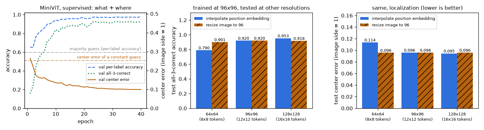
A small ViT with 480,581 parameters reaches a label accuracy of 0.973 and an all-three-labels-correct rate of 0.922 after 40 epochs (validation set). The baseline of always guessing the majority is 0.599. The center of the largest object is off by 0.0994 on average (distance with the image side taken as 1, about 9.5 pixels in a 96-pixel image), which is 39% of the 0.2527 error from always answering the image center. On the left of figure 6-5, accuracy mostly rises by about epoch 10, but center error keeps decreasing slowly to the end. This means putting "where" into a single CLS token is harder than putting "what" into it, which is also why detectors use patch features and object queries rather than the CLS token.
Feeding in a different resolution
This model, trained at 96×96 (a 12×12 grid), is given 64×64 (8×8 grid) and 128×128 (16×16 grid) images of the same scenes. Three methods are compared.
- No interpolation: add the position embeddings as they are.
- Position embedding interpolation: bicubically interpolate the 12×12 grid of position embeddings to 8×8 or 16×16.
- Resize the image to 96 (for comparison): resize the image itself to 96×96 before feeding it in. The position embeddings are left untouched.
해상도 실험 (시험 세트, 같은 장면을 각 해상도로 그린 것)
   64×64  격자  8×8  토큰  64 | 보간 없이: 오류: The size of tensor a (65) must match the size of tensor b (145) at non
            위치 임베딩 보간:        라벨 정확도 0.921 | 세 라벨 모두 0.790 | 중심 오차 0.1136
            그림을 96 으로 바꿔 넣기: 라벨 정확도 0.966 | 세 라벨 모두 0.901 | 중심 오차 0.0957
   96×96  격자 12×12 토큰 144 | 보간 없이: 동작
            위치 임베딩 보간:        라벨 정확도 0.973 | 세 라벨 모두 0.920 | 중심 오차 0.0960
            그림을 96 으로 바꿔 넣기: 라벨 정확도 0.973 | 세 라벨 모두 0.920 | 중심 오차 0.0960
  128×128 격자 16×16 토큰 256 | 보간 없이: 오류: The size of tensor a (257) must match the size of tensor b (145) at no
            위치 임베딩 보간:        라벨 정확도 0.984 | 세 라벨 모두 0.953 | 중심 오차 0.0946
            그림을 96 으로 바꿔 넣기: 라벨 정확도 0.971 | 세 라벨 모두 0.918 | 중심 오차 0.0959
  위치 임베딩을 0 으로 지우면 (96×96): 라벨 정확도 0.905 | 세 라벨 모두 0.736 | 중심 오차 0.3249
| Test resolution | Tokens | No interpolation | Position embedding interpolation | Image resized to 96 |
| 64×64 | 64 | Error | 0.790 · 0.1136 | 0.901 · 0.0957 |
| 96×96 (training resolution) | 144 | Works | 0.920 · 0.0960 | 0.920 · 0.0960 |
| 128×128 | 256 | Error | 0.953 · 0.0946 | 0.918 · 0.0959 |
There are four things to read from the results.
- Without interpolation it cannot be used at all. There are 65 tokens (64 + CLS) but 145 position embeddings, so the addition fails with an error. A convolutional network would not have this problem.
- At the higher resolution (128), performance holds. The all-three-labels rate is 0.953 and the center error 0.0946, no worse than at the training resolution (0.920, 0.0960) and in fact slightly better. It also beats shrinking the image to 96 (0.918). This means the interpolated position embeddings still convey position correctly on a 16×16 grid.
- At the lower resolution (64), performance drops. The all-three-labels rate falls from 0.920 to 0.790 and the center error worsens from 0.0960 to 0.1136. However, enlarging the same 64×64 images to 96 brings it back to 0.901 and 0.0957, so it is not because the images lack information. At 64×64, each patch (8×8) covers a part of the shape 1.5 times wider in each direction, so patch contents differ from those seen in training. The result reflects both the error of position embedding interpolation and this change, and this experiment alone cannot separate the two.
- Erasing the position embeddings loses "where". Zeroing the position embeddings at patch positions worsens the center error from 0.0960 to 0.3249, worse even than always answering the center (0.2527). The kinds of shapes are still recognized, with a label accuracy of 0.905 (0.736 for all three labels). "What" depends on patch contents, and "where" on the position embeddings.
Keep in mind that these are results of changing only the resolution, without fine-tuning. RF-DETR goes a step further, continually changing the resolution during training (multi-scale training, and the resolution knob in NAS) so that a single set of weights works well at many resolutions. This is covered in chapter 11 and chapter 12.
Inspecting the learned position embeddings
The position embeddings started from random values, and nobody told the model which positions neighbor which. After training, we measure how similar positions are to each other. The cosine similarity (1 if two vectors point the same way, 0 if perpendicular, −1 if opposite) between one position's embedding and those of the other 143 positions is drawn on the 12×12 grid.
- Figure: Figure 6-6 Position embeddings of the supervised MiniViT. The star is the reference position, and the color shows how similar each other position's embedding is to it (brighter means more similar).
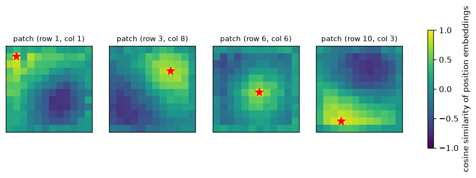
In all four maps, the area around the star is brightest and it darkens with distance. The top-left position resembles top-left positions, and a center position resembles center positions. The model discovered the 2D structure "nearby positions have similar vectors" from the data on its own. This is the same picture the ViT paper (figure 7) reported for large models. And it is why position embedding interpolation works: what varies smoothly over the grid does not go far wrong when the gaps are filled in.
- Note · if the task does not ask about position, the model does not learn position
- While this chapter was being written, the model was first trained only on "what is there". The position embeddings then were structureless noise, unlike figure 6-6. The task did not require position, so there was no reason to learn it. Only after the center coordinates were added as a target did this structure appear. A model learns only as much as the loss demands.
Mini DINO
Now the labels are removed and the same MiniViT is trained with DINO. The components from the previous section are carried over unchanged, just scaled down.
| Item | DINO paper | This chapter's mini DINO |
| Backbone | ViT-S/16 (21 million) | MiniViT, 96×96 / patch 8 (480,000) |
| Output dimension \(K\) | 65,536 | 256 (\(\log K = 5.545\)) |
| Views | 2 global at 224 + several local at 96 | 2 global at 96 + 2 local at 48 |
| Student temperature \(\tau_s\) | 0.1 | 0.1 |
| Teacher temperature \(\tau_t\) | 0.04 → 0.07 | 0.02 (explained below) |
| Teacher EMA rate \(m\) | 0.996 → 1 | 0.99 → 1 |
| Center EMA rate \(m_c\) | 0.9 (the best value in the table in appendix D) | 0.9 |
| Training amount | Hundreds of epochs of ImageNet (about 1.3 million images) | 8,000 images, 3,000 steps × batch 64 (24 epochs' worth) |
The augmentations that create views are random cropping, horizontal flipping and color changes. The color change shuffles the channel order and changes brightness. In Shape World, color is unrelated to the kind of shape, so this tells the model "it is the same image even when the colors differ". Local views are 48×48, giving a 6×6 grid, and enter the same ViT via position embedding interpolation. What was built earlier is used here.
def random_view(images: torch.Tensor, out_size: int, scale: tuple, generator: torch.Generator) -> torch.Tensor:
    """그림마다 무작위 "뷰" 하나를 만든다: 무작위 자르기 + 좌우 뒤집기 + 색 바꾸기 + 잡음.

    images: (B, 3, H, W) 0 – 1  →  (B, 3, out_size, out_size)
    - 자르기: 넓이가 원래의 scale[0] – scale[1] 배, 가로세로 비가 3/4 – 4/3 인 창을 무작위 위치에서 잘라
      out_size 로 크기를 바꾼다 (F.affine_grid + F.grid_sample 로 배치 전체를 한 번에).
    - 색: 채널 순서를 무작위로 섞고(빨강 도형이 파랑 도형이 된다) 밝기를 0.6 – 1.4 배로 바꾼다.
      도형 세상에서 색은 도형의 종류와 무관하므로, "색이 달라도 같은 그림" 이라고 알려 주는 셈이다.
    """
    B, device = len(images), images.device
    rand = lambda *shape: torch.rand(*shape, device=device, generator=generator)
    area = scale[0] + (scale[1] - scale[0]) * rand(B)
    log_ratio = math.log(4 / 3) * (2 * rand(B) - 1)
    width = (area * log_ratio.exp()).sqrt().clamp(max=1.0)  # 창의 너비 · 높이 (그림 한 변 = 1)
    height = (area / log_ratio.exp()).sqrt().clamp(max=1.0)
    center_x = (2 * rand(B) - 1) * (1 - width)  # affine_grid 의 좌표는 −1 – 1: 창이 그림 밖으로 나가지 않게
    center_y = (2 * rand(B) - 1) * (1 - height)
    flip = 1 - 2 * (rand(B) < 0.5).float()  # −1 이면 좌우 뒤집기
    theta = torch.zeros(B, 2, 3, device=device)
    theta[:, 0, 0], theta[:, 0, 2] = width * flip, center_x
    theta[:, 1, 1], theta[:, 1, 2] = height, center_y
    grid = F.affine_grid(theta, (B, 3, out_size, out_size), align_corners=False)
    views = F.grid_sample(images, grid, mode="bilinear", padding_mode="border", align_corners=False)
    permutation = torch.argsort(rand(B, 3), dim=1)  # 그림마다 채널 순서 섞기
    views = torch.gather(views, 1, permutation[:, :, None, None].expand(-1, -1, out_size, out_size))
    views = views * (0.6 + 0.8 * rand(B, 1, 1, 1))
    views = views + 0.02 * torch.randn(views.shape, device=device, generator=generator)
    return views.clamp(0, 1)
class DINOHead(nn.Module):
    """투영 머리: 백본의 CLS 특징 (B, D) → K 차원 점수 (B, K).

    MLP → 병목 차원으로 줄임 → 길이 1 로 정규화 → 가중치 행의 길이도 1 인 선형 층.
    마지막 두 단계 때문에 점수 하나하나는 "두 단위 벡터의 내적" 이라 −1 – 1 사이에 있다.
    그래서 온도 0.1 로 나누면 −10 – 10, 0.02 로 나누면 −50 – 50 의 로짓이 된다.
    이 머리는 사전 학습 때만 쓰고, 학습이 끝나면 버린다 (쓸모 있는 것은 백본이다).
    """

    def __init__(self, dim: int, out_dim: int = 256, hidden: int = 256, bottleneck: int = 64):
        super().__init__()
        self.mlp = nn.Sequential(nn.Linear(dim, hidden), nn.GELU(), nn.Linear(hidden, hidden), nn.GELU(),
                                 nn.Linear(hidden, bottleneck))
        self.last = nn.Linear(bottleneck, out_dim, bias=False)

    def forward(self, x: torch.Tensor) -> torch.Tensor:
        x = F.normalize(self.mlp(x), dim=-1)
        return F.linear(x, F.normalize(self.last.weight, dim=-1))
The loss function follows the equations above exactly. On the teacher side, (t - center) / tau_t applies centering and sharpening, and .detach() cuts the gradient. On the student side, log_softmax computes \(\log P_s\) in a numerically safe way. Cross-entropy minus the teacher's entropy is KL (the decomposition above), so both are logged together to monitor collapse.
def dino_loss(student_out, teacher_out, center, tau_s: float, tau_t: float):
    """DINO 손실: 교사 분포와 학생 분포의 교차 엔트로피를 "서로 다른 뷰" 끼리 계산해 평균한다.

    student_out: 뷰마다의 학생 점수 목록, 각각 (B, K).  teacher_out: 교사 점수 목록(전역 뷰 2개), 각각 (B, K).
    center: (K,) — 교사 점수의 이동 평균. 돌려주는 값: (손실, 교사 분포의 엔트로피 평균, 교사 분포 목록)
    """
    # 교사: 중심을 빼고(centering) 낮은 온도로 나눠(sharpening) 소프트맥스. 기울기는 흘리지 않는다.
    teacher_probs = [((t - center) / tau_t).softmax(dim=-1).detach() for t in teacher_out]
    student_logp = [(s / tau_s).log_softmax(dim=-1) for s in student_out]
    loss, pairs = 0.0, 0
    for i, p_t in enumerate(teacher_probs):
        for j, logp_s in enumerate(student_logp):
            if i == j:  # 같은 뷰끼리는 비교하지 않는다 (그건 그냥 교사를 베끼는 문제가 된다)
                continue
            loss = loss + (-(p_t * logp_s).sum(dim=-1)).mean()  # H(P_t, P_s) = −Σ_k P_t(k) log P_s(k)
            pairs += 1
    entropy = torch.stack([-(p * (p + 1e-12).log()).sum(dim=-1).mean() for p in teacher_probs]).mean()
    return loss / pairs, entropy, teacher_probs
def train_dino(train_images, steps, batch_size=64, dim=96, depth=4, heads=4, out_dim=256, lr=5e-4, weight_decay=0.04,
               tau_s=0.1, tau_t=0.04, momentum=0.99, center_momentum=0.9, use_centering=True, local_views=2,
               seed=0, log=print, name="DINO"):
    """미니 DINO. 라벨은 전혀 쓰지 않는다 (train_images 만 받는다).

    돌려주는 값: (교사 백본, 기록) — 기록은 스텝마다 (손실, 교사 엔트로피, KL, 배치 평균 분포의 엔트로피).
    """
    device = train_images.device
    torch.manual_seed(seed)
    generator = torch.Generator(device=device).manual_seed(seed)
    student = nn.ModuleDict({"backbone": MiniViT(96, 8, dim, depth, heads), "head": DINOHead(dim, out_dim)}).to(device)
    teacher = nn.ModuleDict({"backbone": MiniViT(96, 8, dim, depth, heads), "head": DINOHead(dim, out_dim)}).to(device)
    teacher.load_state_dict(student.state_dict())  # 교사는 학생과 같은 값에서 출발한다
    for p in teacher.parameters():
        p.requires_grad_(False)  # 교사는 기울기로 배우지 않는다. EMA 로만 바뀐다.
    optimizer = torch.optim.AdamW(student.parameters(), lr=lr, weight_decay=weight_decay)
    warmup = max(1, steps // 10)
    center = torch.zeros(out_dim, device=device)
    history = []
    for step in range(steps):
        for group in optimizer.param_groups:  # 학습률: 워밍업 뒤 코사인
            group["lr"] = lr * min((step + 1) / warmup, 0.5 * (1 + math.cos(math.pi * step / steps)))
        index = torch.randint(len(train_images), (batch_size,), device=device, generator=generator)
        images = to_float(train_images[index])
        # 같은 그림에서 뷰를 여러 개: 크게 자른 전역 뷰 2개(96×96) + 작게 자른 지역 뷰 local_views 개(48×48)
        global_views = [random_view(images, 96, (0.5, 1.0), generator) for _ in range(2)]
        local_view_list = [random_view(images, 48, (0.15, 0.5), generator) for _ in range(local_views)]
        with torch.no_grad():  # 교사는 전역 뷰만 본다
            teacher_out = [teacher["head"](teacher["backbone"](v)) for v in global_views]
        # 학생은 모든 뷰를 본다. 48×48 뷰는 격자가 6×6 이라 위치 임베딩이 보간되어 들어간다.
        student_out = [student["head"](student["backbone"](v)) for v in global_views + local_view_list]
        loss, entropy, teacher_probs = dino_loss(student_out, teacher_out, center if use_centering else 0.0, tau_s, tau_t)
        optimizer.zero_grad()
        loss.backward()
        torch.nn.utils.clip_grad_norm_(student.parameters(), 3.0)
        optimizer.step()
        with torch.no_grad():
            # 교사 = 학생의 지수 이동 평균. m 은 코사인을 따라 momentum → 1 로 올라간다.
            m = 1 - (1 - momentum) * 0.5 * (1 + math.cos(math.pi * step / steps))
            for p_t, p_s in zip(teacher.parameters(), student.parameters()):
                p_t.mul_(m).add_(p_s.detach(), alpha=1 - m)
            # 중심 = 교사 점수의 배치 평균을 이동 평균한 것
            center = center_momentum * center + (1 - center_momentum) * torch.cat(teacher_out).mean(dim=0)
            mean_probs = torch.cat(teacher_probs).mean(dim=0)  # 배치 전체가 K 개 차원을 얼마나 고르게 쓰는가
            marginal_entropy = -(mean_probs * (mean_probs + 1e-12).log()).sum().item()
        history.append((loss.item(), entropy.item(), loss.item() - entropy.item(), marginal_entropy))
        if (step + 1) % max(1, steps // 5) == 0 or step == 0:
            log(f"  [{name}] 스텝 {step + 1:5d} | 손실 {loss.item():.3f} | 교사 엔트로피 {entropy.item():.3f}"
                f" | KL {loss.item() - entropy.item():.3f} | 배치 평균 분포의 엔트로피 {marginal_entropy:.3f}")
    return teacher["backbone"].eval(), np.array(history)
There are three places to look in the training loop.
- The teacher sees only the global views, inside
torch.no_grad(); the student sees all views. -
optimizer.step()changes only the student. After that, every teacher parameter is updated withp_t.mul_(m).add_(p_s, alpha=1 - m), that is, \(\theta_t \leftarrow m\theta_t + (1 - m)\theta_s\). - The center
centeris also updated with a moving average of the same form. It is not a value learned through the loss.
Pretraining is done twice, each time with a different kind of unlabeled image: (a) scenes: 8,000 ordinary Shape World images with 1–4 shapes; (b) single shapes: 8,000 images with just one shape. Neither uses labels. Why they were split in two becomes clear in the results.
- Note · why the teacher temperature was lowered to 0.02
- The first run used the DINO paper's 0.04. It did not collapse, but the teacher's distribution sharpened slowly, and even after 3,000 steps the backbone trained on (b) was indistinguishable from random initialization on the linear classifier asking for the kind of shape (only the object-count task improved slightly). Lowering it to 0.02 let training progress within the same number of steps. Appendix D of the paper also shows that 0.02 is a working value (starting above 0.06 collapses). Note that this chapter's figures come from one setting chosen after trying several. You can check for yourself with
--tau-t 0.04.
Watching collapse directly
Along with the two normal mini DINO runs, two short experiments (300 steps) are run with one component removed each. Centering off keeps the center \(c\) at 0 always, and sharpening off raises the teacher temperature to 1.0. Three values are logged at every step: the entropy of the teacher's distribution \(\mathrm{Ent}(P_t)\) (how spread out one image's distribution is), KL (how different teacher and student are), and the entropy of the distribution averaged over the whole batch (how evenly the batch uses the \(K\) slots).
미니 DINO (라벨 없이): 스텝 3000, 배치 64, 교사 온도 0.02
  [DINO · 장면] 스텝     1 | 손실 3.186 | 교사 엔트로피 1.339 | KL 1.847 | 배치 평균 분포의 엔트로피 1.389
  [DINO · 장면] 스텝   600 | 손실 2.464 | 교사 엔트로피 1.773 | KL 0.691 | 배치 평균 분포의 엔트로피 2.974
  [DINO · 장면] 스텝  1200 | 손실 1.790 | 교사 엔트로피 0.939 | KL 0.851 | 배치 평균 분포의 엔트로피 2.401
  [DINO · 장면] 스텝  1800 | 손실 1.439 | 교사 엔트로피 0.299 | KL 1.140 | 배치 평균 분포의 엔트로피 2.444
  [DINO · 장면] 스텝  2400 | 손실 1.237 | 교사 엔트로피 0.145 | KL 1.092 | 배치 평균 분포의 엔트로피 2.265
  [DINO · 장면] 스텝  3000 | 손실 1.117 | 교사 엔트로피 0.235 | KL 0.883 | 배치 평균 분포의 엔트로피 2.348
  [DINO · 도형 하나] 스텝     1 | 손실 3.105 | 교사 엔트로피 1.273 | KL 1.832 | 배치 평균 분포의 엔트로피 1.291
  [DINO · 도형 하나] 스텝   600 | 손실 3.511 | 교사 엔트로피 2.790 | KL 0.721 | 배치 평균 분포의 엔트로피 3.879
  [DINO · 도형 하나] 스텝  1200 | 손실 2.288 | 교사 엔트로피 1.284 | KL 1.004 | 배치 평균 분포의 엔트로피 3.112
  [DINO · 도형 하나] 스텝  1800 | 손실 1.153 | 교사 엔트로피 0.245 | KL 0.908 | 배치 평균 분포의 엔트로피 2.617
  [DINO · 도형 하나] 스텝  2400 | 손실 1.095 | 교사 엔트로피 0.258 | KL 0.837 | 배치 평균 분포의 엔트로피 2.709
  [DINO · 도형 하나] 스텝  3000 | 손실 1.012 | 교사 엔트로피 0.235 | KL 0.777 | 배치 평균 분포의 엔트로피 2.579
미니 DINO 학습 둘 430.7초
  [centering 끔] 스텝     1 | 손실 3.105 | 교사 엔트로피 1.273 | KL 1.832 | 배치 평균 분포의 엔트로피 1.291
  [centering 끔] 스텝    60 | 손실 0.026 | 교사 엔트로피 0.017 | KL 0.009 | 배치 평균 분포의 엔트로피 0.017
  [centering 끔] 스텝   120 | 손실 0.005 | 교사 엔트로피 0.000 | KL 0.005 | 배치 평균 분포의 엔트로피 0.000
  [centering 끔] 스텝   180 | 손실 0.004 | 교사 엔트로피 0.000 | KL 0.004 | 배치 평균 분포의 엔트로피 0.000
  [centering 끔] 스텝   240 | 손실 0.003 | 교사 엔트로피 0.000 | KL 0.003 | 배치 평균 분포의 엔트로피 0.000
  [centering 끔] 스텝   300 | 손실 0.003 | 교사 엔트로피 0.000 | KL 0.003 | 배치 평균 분포의 엔트로피 0.000
  [sharpening 끔] 스텝     1 | 손실 6.163 | 교사 엔트로피 5.537 | KL 0.627 | 배치 평균 분포의 엔트로피 5.537
  [sharpening 끔] 스텝    60 | 손실 5.547 | 교사 엔트로피 5.545 | KL 0.002 | 배치 평균 분포의 엔트로피 5.545
  [sharpening 끔] 스텝   120 | 손실 5.545 | 교사 엔트로피 5.545 | KL 0.000 | 배치 평균 분포의 엔트로피 5.545
  [sharpening 끔] 스텝   180 | 손실 5.545 | 교사 엔트로피 5.545 | KL 0.000 | 배치 평균 분포의 엔트로피 5.545
  [sharpening 끔] 스텝   240 | 손실 5.545 | 교사 엔트로피 5.545 | KL 0.000 | 배치 평균 분포의 엔트로피 5.545
  [sharpening 끔] 스텝   300 | 손실 5.545 | 교사 엔트로피 5.545 | KL 0.000 | 배치 평균 분포의 엔트로피 5.545
끈 실험 둘 41.3초, log K = log 256 = 5.545
- Figure: Figure 6-7 Left: teacher entropy. Middle: KL (= loss − entropy). Right: entropy of the batch-averaged distribution. The gray dash-dot line is \(\log K = 5.545\). Curves are 25-step moving averages.
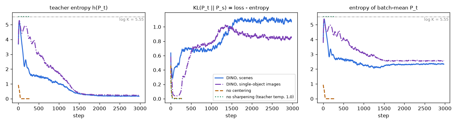
The two collapses summarized in the table earlier appear exactly.
- With centering off, it concentrates on one slot. In just 60 steps the teacher entropy reaches 0.017, then 0.000 at 120 steps, and KL drops to 0.005. Even the entropy of the batch-averaged distribution being 0 means every image in the batch picked the same single slot. With the loss near 0 it is easy to mistake this for "training going well", but the model is just giving the same slot for every image.
- With sharpening off, it becomes uniform. The teacher entropy is 5.537 from the start and reaches \(\log K = 5.545\) by step 60, while KL becomes 0.002 and then 0.000. The teacher answers "don't know" for every image and the student copies it. The loss does not budge from \(\log K\).
- With both on, it stays in between. After 3,000 steps both runs have a teacher entropy of 0.235 and KL of 0.883 (scenes) and 0.777 (single shapes). Each image picks nearly one slot clearly (low teacher entropy), but the batch as a whole spreads across several slots (batch-averaged entropy of 2.348 and 2.579, equivalent to using roughly \(e^{2.35} \approx 10\) to \(e^{2.58} \approx 13\) slots evenly). And KL does not go to 0, because the teacher's answer differs per image and the student cannot know it in advance.
The lesson of this experiment is that the loss value alone cannot distinguish healthy training from collapse. In self-supervised learning, look not at whether the loss goes down but at where entropy and KL settle.
Measuring features with a linear classifier
Not collapsing does not guarantee that anything useful was learned. Backbones from self-supervised learning are measured with linear probe evaluation: freeze the backbone (leave its weights unchanged) and train only a single linear layer on its features with labels. The score reflects only what a single linear layer can solve, so it is a test of how readily extractable the answer is from the features. The features are 192-dimensional, concatenating the CLS output and the mean of the patch outputs. Three questions are asked.
- ① Which shapes are in the scene? (the same multi-label task as in supervised training)
- ② How many objects are in the scene? (one of 1–4)
- ③ What is the shape in a single-shape image? (one of circle, square, triangle)
@torch.no_grad()
def extract_features(backbone, images_uint8, batch_size=250) -> torch.Tensor:
    """얼린 백본의 특징: CLS 토큰과 패치 토큰 평균을 이어 붙인다. (그림 수, 2D)"""
    backbone.eval()
    features = []
    for i in range(0, len(images_uint8), batch_size):
        tokens = backbone.forward_tokens(to_float(images_uint8[i : i + batch_size]))  # (B, 1 + N, D)
        features.append(torch.cat([tokens[:, 0], tokens[:, 1:].mean(dim=1)], dim=1))
    return torch.cat(features)

def linear_probe(train_features, train_targets, test_features, epochs=300, lr=1e-2, seed=0) -> torch.Tensor:
    """얼린 특징 위에 선형 층 하나만 학습하고 (라벨은 여기서만 쓴다), 시험 특징에 대한 로짓을 돌려준다.

    train_targets 가 실수 (n, 3) 이면 다중 라벨 문제로 보고 BCE 를,
    정수 (n,) 이면 여러 클래스 중 하나를 고르는 문제로 보고 소프트맥스 교차 엔트로피를 쓴다.
    특징은 학습 세트의 평균 · 표준편차로 정규화한다. 선형 층 하나로 풀리는 만큼만 점수가 나오므로,
    "특징 안에 답이 얼마나 꺼내기 쉬운 꼴로 들어 있는가" 를 재는 시험이 된다.
    """
    torch.manual_seed(seed)
    mean, std = train_features.mean(0, keepdim=True), train_features.std(0, keepdim=True) + 1e-6
    x_train, x_test = (train_features - mean) / std, (test_features - mean) / std
    multi_label = train_targets.is_floating_point()
    n_outputs = train_targets.shape[1] if multi_label else int(train_targets.max()) + 1
    probe = nn.Linear(x_train.shape[1], n_outputs).to(x_train.device)
    optimizer = torch.optim.AdamW(probe.parameters(), lr=lr, weight_decay=1e-2)
    for _ in range(epochs):  # 특징이 작아서 전체를 한 배치로 쓴다
        logits = probe(x_train)
        loss = F.binary_cross_entropy_with_logits(logits, train_targets) if multi_label else F.cross_entropy(logits, train_targets)
        optimizer.zero_grad()
        loss.backward()
        optimizer.step()
    with torch.no_grad():
        return probe(x_test)
선형 분류기 (얼린 특징 192차원, 라벨 달린 학습 그림 4000장, 시험 1000장)
  백본                         | ① 장면의 도형 종류: 라벨 정확도 · 세 라벨 모두 | ② 장면의 객체 수 | ③ 도형 하나의 종류
  무작위 초기화 (시드 1)             | 0.712 · 0.312 | 0.671 | 0.593
  무작위 초기화 (시드 2)             | 0.721 · 0.331 | 0.663 | 0.592
  미니 DINO · 장면               | 0.737 · 0.361 | 0.754 | 0.729
  미니 DINO · 도형 하나            | 0.810 · 0.521 | 0.713 | 0.934
  centering 끈 DINO           | 0.729 · 0.345 | 0.688 | 0.622
  sharpening 끈 DINO          | 0.721 · 0.327 | 0.696 | 0.646
  지도 학습 백본 (참고)              | 0.971 · 0.914 | 0.729 | 0.999
  픽셀 (8×8 평균, 432차원)         | 0.627 · 0.243 | 0.511 | 0.450
  늘 많은 쪽으로 찍기                | 0.599 ·   —   | 0.269 | 0.351
GPU 메모리 최대 사용량 1533 MiB
- Figure: Figure 6-8 Linear classifier accuracy on frozen features (test set). From the left, tasks ①, ② and ③. The black dash-dot line is the accuracy of always guessing the majority.
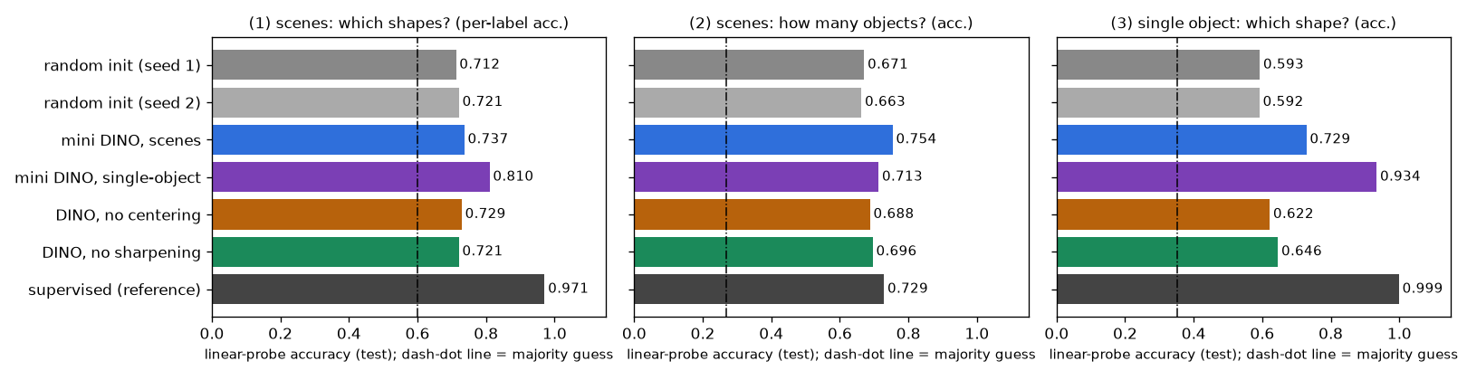
Let us read the table row by row.
- Even a randomly initialized backbone is not zero. It scores 0.71–0.72, 0.66–0.67 and 0.59 on the three tasks, higher not only than always guessing the majority (0.599, 0.269, 0.351) but also than a linear classifier on raw pixels (0.627, 0.511, 0.450). An untrained network still produces features that mix the image in various ways, and some of them happen to be useful. So the baseline for comparison should be this row, not "guessing". The difference between the two rows with different seeds (0.001–0.009) gives a sense of how much this experiment fluctuates by chance.
- A collapsed DINO is no different from random initialization. On task ① it scores 0.729 and 0.721, the same as random initialization (0.712, 0.721), and on ② and ③ it is only 0.02–0.05 higher (apparently traces of the weights moving a little during the few dozen steps before collapse). The loss was the lowest, yet nothing was learned.
- Mini DINO trained on scenes learned "how many". Object count (②) rose from 0.67 to 0.754, higher even than the backbone trained with labels (0.729). The single-shape kind (③) also rose from 0.59 to 0.729. But the kind of shapes in the scene (①) itself is 0.737, only 0.02 higher than random initialization (0.712, 0.721), a difference that barely exceeds the seed-to-seed fluctuation.
- Mini DINO trained on single-shape images learned "what shape". It gets the single-shape kind (③) right 0.934 of the time. Random initialization gets 0.59, and the backbone trained with labels 0.999. Features obtained without a single label nearly separate the three shapes with just one linear layer on top. These features also transfer to scenes never seen before, raising ① from 0.72 to 0.810 (all three labels from 0.31–0.33 to 0.521). Object count (②) is 0.713, lower than the scene-trained one (0.754).
- The backbone trained with labels is much better at its own tasks. ① is 0.971 and ③ is 0.999. Naturally, since it learned exactly what the labels ask. On the other hand, object count (②), which the labels never asked about, is 0.729, slightly lower than the mini DINO trained on scenes without labels (0.754). Labels produce features specialized for what those labels ask; self-supervised learning produces features not tied to a particular task. In this small experiment, however, the extent of that generality is narrow.
Same method, same model, same augmentations, yet what was learned changed with nothing but the kind of unlabeled images. The reason lies in DINO's objective. DINO puts into the features what stays unchanged between two views. When a scene with several shapes is cropped and recolored, the most salient thing common to both views is roughly how many shapes there are and how large they are. The kind of shape is a subtler cue. In an image with only one shape, what remains after cropping and recoloring is essentially just the shape's form, so distinguishing images requires looking at the form. (This is an interpretation of the experiment's results and has not been separately verified.)
- Key point · what self-supervised learning learns is decided by the data and augmentations
- The DINO paper trained on ImageNet. It is a classification dataset with one label per photo, so many photos have a single main object. The DINOv2 paper also treats data as important: it built the curated LVD-142M instead of using internet images as is, and reports that training on uncurated images worsens results on most benchmarks (table 2). And the scale is different. This chapter's mini DINO saw 8,000 images 24 times, while DINOv2 trained a 1-billion-parameter model on 142 million images and distilled it. Do not mistake a small experiment's results for the quality of the real DINOv2. The difference is shown directly at the end of this chapter.
Where does the CLS token look?
The weights the CLS token gives each patch in the last block's self-attention (averaged over the 4 heads) are drawn as a 12×12 map. It shows which patches the CLS token draws information from to summarize the whole image.
- Figure: Figure 6-9 Row 1: test images. Row 2: supervised MiniViT. Row 3: mini DINO trained on scenes (teacher). Row 4: mini DINO trained on single-shape images (teacher). Brighter means the CLS token looks at that patch more.
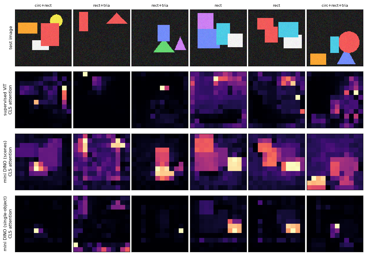
The CLS token of the supervised model (row 2) does not look evenly over the shapes. Its weight is concentrated on a few scattered patches, some on shape edges and some on background. By the last block, the needed information may already have been moved into various tokens by the earlier blocks, so it is hard to say from a single last-layer attention map that "the model decided by looking here". Mini DINO (rows 3 and 4) is different: the bright spots are mostly on the shapes. The scene-trained one looks broadly at one or two shapes and their surroundings, and the one trained on single-shape images concentrates on a narrow part of one shape (sometimes drifting into a background corner, as in the second image). There were no labels and no instruction to "look at the shapes", yet the CLS token looks toward the objects. The DINO paper reported that the self-attention maps of self-supervised ViTs reveal scene layout and object boundaries; this is a small version of that property. That said, this was observed by eye on six images and not measured numerically.
Patch features of the real DINOv2
Finally, the released DINOv2 ViT-S/14 weights are downloaded and Shape World images are fed in. DINOv2 was trained on photos and has never seen images like Shape World. Will its patch features still distinguish the shapes? This part is an optional script separate from the main exercises, code/ch06_dinov2_features.py. It needs the transformers package, which is not in requirements.txt, and an internet connection (to download about 88 MB of weights).
Rendering the same scenes at 224×224 gives \(224 / 14 = 16\), so each image yields \(16 \times 16 = 256\) patch features (each 384-dimensional). Two things are done with these features.
- Patch classification. With the backbone frozen, a single linear layer is trained on the patch features to predict "background, circle, square or triangle" for each patch. A patch's ground truth is whatever occupies the most area within it. This is the most direct test of the ability a detector wants from its backbone. It is compared against the same architecture, randomly initialized.
- Principal component analysis (PCA). The three directions of greatest spread in the 384-dimensional patch features are found and colored red, green and blue. Patches with similar features get similar colors. Following the procedure used in figure 1 of the DINOv2 paper, the background is also separated by the sign of the first principal component, and principal components are recomputed from the remaining patches only.
@torch.no_grad()
def patch_features(model, images_uint8: torch.Tensor, device: str, batch_size: int = 100):
    """DINOv2 의 마지막 층 출력을 꺼낸다.

    images_uint8: (n, 3, 224, 224) → CLS (n, 384), 패치 특징 (n, 256, 384).
    출력 토큰 열은 [CLS, 패치 256개] 순서다 (이 가중치는 레지스터 토큰이 없는 판이다).
    """
    cls_list, patch_list = [], []
    for i in range(0, len(images_uint8), batch_size):
        x = images_uint8[i : i + batch_size].to(device).float() / 255.0
        x = (x - IMAGENET_MEAN.to(device)) / IMAGENET_STD.to(device)
        tokens = model(pixel_values=x).last_hidden_state  # (B, 1 + 256, 384)
        cls_list.append(tokens[:, 0].cpu())
        patch_list.append(tokens[:, 1:].cpu())
    return torch.cat(cls_list), torch.cat(patch_list)
def patch_labels(dataset: ShapesDataset, patch_size: int = 14) -> torch.Tensor:
    """패치마다의 정답: 0 배경, 1 원, 2 사각형, 3 삼각형. (n, 격자²)

    패치 안의 픽셀을 "배경 · 원 · 사각형 · 삼각형" 넷으로 나눠 세어, 가장 많은 것을 그 패치의 라벨로 한다.
    """
    grid = dataset.size // patch_size
    labels = torch.zeros(len(dataset), grid * grid, dtype=torch.int64)
    for i, target in enumerate(dataset.targets):
        pixel_class = torch.zeros(dataset.size, dataset.size, dtype=torch.int64)
        for mask, cls in zip(target["masks"], target["labels"]):
            pixel_class[mask] = int(cls) + 1  # 보이는 부분만 True 인 마스크라 겹쳐도 덮어쓰지 않는다
        one_hot = F.one_hot(pixel_class, NUM_CLASSES + 1).permute(2, 0, 1).float()[None]  # (1, 4, S, S)
        counts = F.avg_pool2d(one_hot, patch_size)[0]  # (4, 격자, 격자): 패치 안에서 각 종류가 차지하는 비율
        labels[i] = counts.argmax(dim=0).flatten()
    return labels
def pca_colors(features: torch.Tensor) -> np.ndarray:
    """(패치 수, D) 특징 → (패치 수, 3) 색. 앞의 세 주성분을 성분별로 0 – 1 로 늘려 RGB 로 쓴다.

    주성분 분석은 특징이 가장 크게 퍼진 방향부터 차례로 찾는다. 비슷한 특징을 가진 패치는 비슷한 색이 된다.
    """
    centered = features - features.mean(dim=0, keepdim=True)
    _, _, vh = torch.linalg.svd(centered, full_matrices=False)  # vh 의 줄이 주성분 방향
    projected = centered @ vh[:3].T  # (패치 수, 3)
    low, high = projected.min(dim=0).values, projected.max(dim=0).values
    return ((projected - low) / (high - low)).numpy()

def first_component_foreground(features: torch.Tensor):
    """첫 주성분 값과, 그 부호로 가른 "도형 패치" 표시. 수가 적은 쪽을 도형으로 본다 (그림의 대부분은 배경이다)."""
    centered = features - features.mean(dim=0, keepdim=True)
    _, _, vh = torch.linalg.svd(centered, full_matrices=False)
    first = centered @ vh[0]
    positive = first > 0
    if positive.float().mean() > 0.5:  # 주성분의 부호는 임의다: 적은 쪽이 True 가 되게 뒤집는다
        positive = ~positive
    return first, positive
장치: cuda

facebook/dinov2-small: 매개변수 22,056,576개, 층 12, 차원 384, 머리 6, 패치 14, 위치 임베딩 (1, 1370, 384)
패치 라벨: 학습 153,600개, 시험 76,800개, 시험 패치 중 배경 0.863
  사전 학습된 DINOv2        패치 분류 정확도 0.968 | 배경이 아닌 패치만 0.907
  무작위 초기화 (같은 구조)      패치 분류 정확도 0.922 | 배경이 아닌 패치만 0.452
  늘 배경이라고 찍기           패치 분류 정확도 0.863 | 배경이 아닌 패치만 0.000
  사전 학습된 DINOv2        첫 주성분의 부호만으로 배경/도형 가르기: 정답과 일치 0.726
  무작위 초기화 (같은 구조)      첫 주성분의 부호만으로 배경/도형 가르기: 정답과 일치 0.952
- Figure: Figure 6-10 Row 1: input (224×224). Row 2: PCA of DINOv2 patch features (all patches). Row 3: DINOv2, PCA of only the patches remaining after separation by the first principal component (the rest in black). Rows 4 and 5: the same procedure applied to a randomly initialized ViT of the same architecture. The colors themselves have no meaning; same color = similar features.
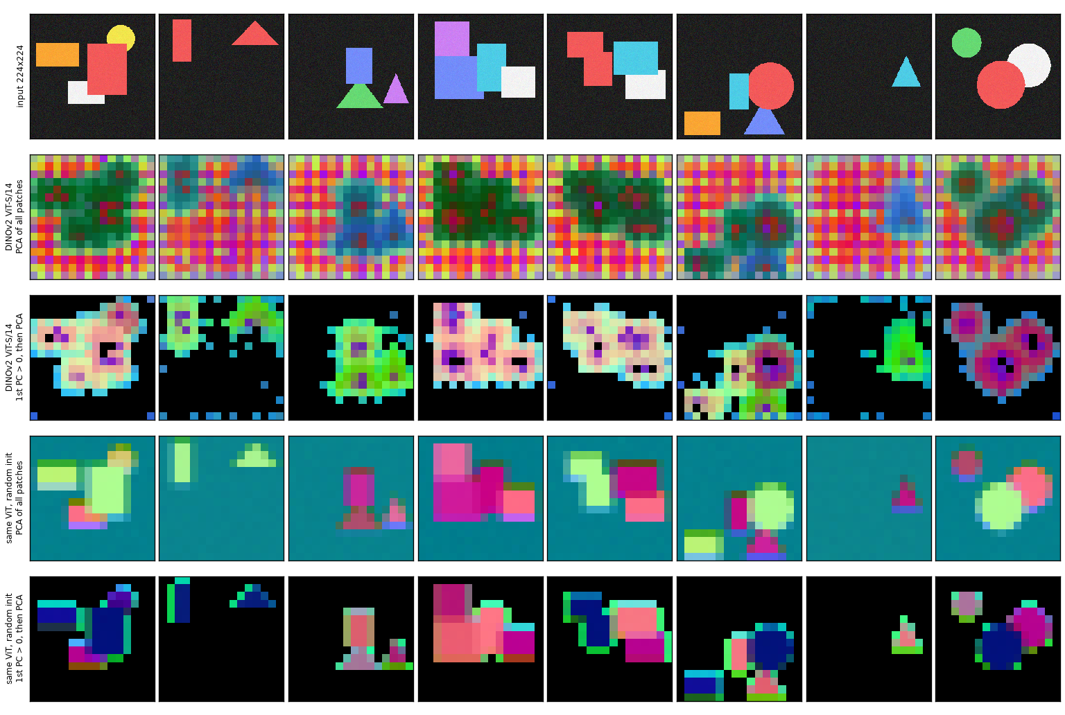
First, the numbers.
- Patch classification. 86.3% of test patches are background, so the overall accuracy (0.968 vs 0.922) looks like a small gap. Looking only at patches on shapes, pretrained DINOv2 scores 0.907 and the randomly initialized same architecture 0.452. Random-initialization features can tell "something is here", but cannot even half the time tell whether it is a circle, square or triangle. DINOv2 saw only photos, was trained without labels, and is seeing Shape World images for the first time. Yet with just one linear layer on top it identifies the kind of shape per patch 91% of the time.
- Separating the background with the first principal component. Here, conversely, random initialization (0.952) beats DINOv2 (0.726). Shape World has dark backgrounds and bright shapes, so the background separates by brightness alone, and the direction of greatest spread in the random-initialization features appears to be exactly brightness and color (the colors in row 4 follow the input colors directly). On the DINOv2 side, background patches around the shapes also cross over to the shape side (in row 3 the shapes look swollen by one or two cells). This also means that patch features carry the surrounding context, not just the patch's own pixels. The "first principal component = main object" that the DINOv2 paper showed on photos was not reproduced as cleanly on these toy images. This is recorded as is.
What to read from figure 6-10 is what the colors follow.
- The colors of random initialization (rows 4 and 5) follow the input colors. Red shapes, whatever their form, are painted one color, and light-blue shapes another. The features are little more than a slight mix of pixel values.
- The colors of DINOv2 (row 3) are independent of the input colors and tend to follow the kind of shape. In the first image the orange, red and white squares are all pale pink; in the last image the green, white and red circles are all purple; and the triangles are green. It is not clean: the squares in the second and third images are a greenish hue similar to the triangles. The 0.907 above is the numerical measure of this visually observed tendency.
- DINOv2's background (row 2) has a grid pattern. This means the features of empty background patches vary regularly with position. Photos rarely have such wide, uniform backgrounds. It may be related to the problem of "low-information background patches" discussed in the registers paper, but this experiment does not confirm that.
What mini DINO barely achieved from 8,000 single-shape images, the real DINOv2 achieves on each individual patch of images it has never seen. This is exactly what a detector wants. If the patch features alone can say "this is part of a triangle", the job of the decoder on top becomes much easier. This is why RF-DETR starts from these weights rather than random ones, and the background to the 2 AP gained just by swapping the backbone in tables 5 and 6 of the paper.
Summary
- ViT cuts an image into \(p \times p\) patches, linearly projects each patch, and feeds the resulting \(N = (H/p)(W/p)\) tokens into a pre-norm Transformer encoder. Patch embedding is the same computation as a single convolution with kernel and stride \(p\).
- The first row of the output (CLS) summarizes the whole image, and the remaining \(N\) rows are patch features. Detection uses the feature map made by folding the patch features into a grid.
- ViT-S (12 layers, \(D = 384\)) has about 22 million parameters, most of them in the blocks. Doubling the dimension multiplies them by about 4.
- One block's compute is roughly \(12ND^2 + 2N^2D\). The token count is set by the ratio \(H/p\) of resolution to patch size; doubling that ratio gives 4 times the tokens and 16 times the attention pairs.
- Only two sets of weights are tied to the image size: the position embedding and the patch embedding. Position embeddings are reshaped into a 2D grid and interpolated, and the patch embedding is resized FlexiViT-style (chapter 12).
- ViT has a weak inductive bias and needs large datasets. So it starts from pretrained weights and is fine-tuned.
- DINO, without labels, makes the student's distribution follow the EMA teacher's distribution for different views of the same image. The loss is cross-entropy, and gradients flow only to the student.
- Collapse has two forms, one-slot concentration (entropy 0) and uniform (entropy \(\log K\)), and both drive KL to 0. Centering prevents the former and sharpening the latter.
- DINOv2 applied image-level (DINO) + patch-level (iBOT) losses to 142 million curated images and distilled a large model into small ones. Its good patch features made it RF-DETR's backbone, and in the paper's ablations swapping in this backbone alone gave +2 AP.
- In this chapter's experiments, what mini DINO learned depended on the kind of unlabeled images. Trained on scenes, object count could be read from the frozen features; trained on single-shape images, the kind of shape could. What self-supervised learning learns is decided by the data and augmentations, and its quality comes from scale.
The detector's eyes are now ready. Feed in an image and out comes one feature vector per patch, and even though these features were learned without labels, they distinguish objects from background and one kind of object from another. But a feature map is not yet the answer. What we want is a list of boxes and classes: "one circle here, one triangle there". How many there will be also differs per image. Chapter 7 builds DETR, the first detector to tackle this problem head-on with a Transformer. It treats detection as "a set prediction problem" and outputs boxes with object queries and Hungarian matching, with neither anchors nor NMS.
Review questions
- 1. Token count: RF-DETR L uses resolution 704 and patch size 16 (table 7 of the paper). How many patch tokens are there? Compared with nano (384, patch 16), by what factor do the token count and the number of self-attention pairs grow?
- \(704 / 16 = 44\), so \(N = 44^2 = 1936\). Nano has \(24^2 = 576\), so tokens grow \(1936 / 576 \approx 3.36\) times and pairs \(3.36^2 \approx 11.3\) times. The resolution only went up 1.83 times.
- 2. Parameter count: count the parameters of this chapter's
MiniViT(96×96, patch 8, \(D = 96\), 4 layers, MLP ratio 4, 5 outputs) part by part. Does it match the 480,581 in the run output? -
- Patch embedding: \(3 \cdot 8 \cdot 8 \cdot 96 + 96 = 18{,}528\)
- CLS token 96, position embedding \((144 + 1) \cdot 96 = 13{,}920\)
- One block: two layer normalizations \(2 \cdot 192 = 384\), qkv \(96 \cdot 288 + 288 = 27{,}936\), output projection \(96 \cdot 96 + 96 = 9{,}312\), MLP \(96 \cdot 384 + 384 = 37{,}248\) and \(384 \cdot 96 + 96 = 36{,}960\) → total \(111{,}840\). Four blocks: \(447{,}360\)
- Final layer normalization 192, head \(96 \cdot 5 + 5 = 485\)
- Total: \(18{,}528 + 96 + 13{,}920 + 447{,}360 + 192 + 485 = 480{,}581\). It matches.
- 3. EMA by hand: one teacher weight is \(\theta_t = 0.5\) and the student's is \(\theta_s = 1.5\). After one update with \(m = 0.99\), what is \(\theta_t\)? After 100 updates with the student staying at 1.5? (\(0.99^{100} \approx 0.366\))
- Once: \(0.99 \cdot 0.5 + 0.01 \cdot 1.5 = 0.51\). The remaining gap shrinks by a factor of 0.99 per step, so after 100 steps it is \(1 \cdot 0.99^{100} \approx 0.366\), that is, \(\theta_t \approx 1.5 - 0.366 = 1.134\). Even after 100 steps, the teacher has covered only 63% of the distance to the student.
- 4. Temperature: with scores \(a = (1, 0)\), compute the softmax at temperatures \(\tau = 1\), \(0.5\) and \(0.1\). (\(e^1 \approx 2.718\), \(e^2 \approx 7.389\), \(e^{10} \approx 22026\))
- \(\tau = 1\): \((2.718, 1)/3.718 = (0.731, 0.269)\). \(\tau = 0.5\): the scores become \((2, 0)\), giving \((7.389, 1)/8.389 = (0.881, 0.119)\). \(\tau = 0.1\): the scores become \((10, 0)\), giving \((22026, 1)/22027 \approx (0.99995, 0.00005)\). The lower the temperature, the closer to one-hot.
- 5. Recognizing collapse: a mini DINO with output dimension \(K = 256\) was run twice, and the logs at the end of training were (a) teacher entropy 5.545, KL 0.000 and (b) teacher entropy 0.000, KL 0.001. What state is each in? What was most likely left out? (\(\ln 256 \approx 5.545\))
- Both have KL of 0, so both have collapsed. (a) has entropy \(\log K\), so it is collapse into a uniform distribution for every image, most likely caused by a teacher temperature that is too high (no sharpening). (b) has entropy 0, so it is collapse where every image concentrates on one slot, most likely because centering was left out. This is exactly what this chapter's experiments showed.
- 6. Position embedding interpolation: a single-valued position embedding has three cells in a row, \([2,\ 4,\ 8]\) (\(g = 3\)). Shrinking it to two cells (\(g' = 2\)) with bilinear interpolation, what are the values? Use the formula from the text, \(u_i = (i + 0.5)\cdot g/g' - 0.5\).
- \(u_0 = 0.5 \cdot 1.5 - 0.5 = 0.25\): a quarter of the way between cell 0 (value 2) and cell 1 (value 4), so \(0.75 \cdot 2 + 0.25 \cdot 4 = 2.5\). \(u_1 = 1.5 \cdot 1.5 - 0.5 = 1.75\): three quarters of the way between cell 1 (value 4) and cell 2 (value 8), so \(0.25 \cdot 4 + 0.75 \cdot 8 = 7\). The answer is \([2.5,\ 7]\).
- 7. Same token count, different method: ViT-S is used at 384×384 with patch 16, and we want to enlarge images to 768×768. How do (a) keeping the patch size at 16 and (b) enlarging the patch size to 32 differ in token count, block compute and weights that must change?
- (a) The grid becomes \(768/16 = 48\), so tokens go \(576 \to 2304\) (4 times) and attention pairs 16 times. \(N = 6D = 2304\), the point where the quadratic and linear terms of a block are equal, and block compute grows about 6.4 times. The position embeddings must be interpolated from 24×24 to 48×48, while the patch embedding is used as is. (b) The grid stays at \(768/32 = 24\), so the token count and block compute do not change and the position embeddings are used as is. Instead, the patch embedding kernel must change from 16×16 to 32×32 (a FlexiViT-style transformation), and each patch covers 4 times the area of the original image. Going by the observation in appendix L of the RF-DETR paper, one can expect (b)'s accuracy to be similar to that at 384/16.
- 8. Why no gradients flow to the teacher: explain what would happen if DINO's loss \(\mathrm{CE}(P_t, P_s)\) were also differentiated with respect to the teacher's weights and the teacher trained together by gradient descent.
- If both teacher and student moved to reduce the loss, the easiest way to drive it to 0 would be for both to output "the same single slot for every image" together (entropy 0, KL 0). For the teacher to serve as a target, it must not be dragged around by the loss. That is why the teacher side gets a stop-gradient and changes only slowly through the EMA. Centering and sharpening are likewise not learned through the loss but are operations applied externally to the teacher's output.
- Try changing it yourself
- Run mini DINO twice as long with
python ch06_vit.py --dino-steps 6000and see how the linear classifier table changes, and see what happens when--tau-t 0.04raises the teacher temperature to the DINO paper's value. Also predict, then check, what changes if channel shuffling is removed fromrandom_view(no color changes). Remember that augmentations decide "what to treat as the same". Also see what happens to the curves in figure 6-7 ifmomentumintrain_dinois lowered from 0.99 to 0.9 so the teacher follows the student quickly.
See also
Favorite site
- 06. Vision Transformer and DINOv2
- code/ch06_vit.py
- code/ch06_dinov2_features.py
- An Image is Worth 16x16 Words: Transformers for Image Recognition at Scale (ViT, arXiv:2010.11929)
- Emerging Properties in Self-Supervised Vision Transformers (DINO, arXiv:2104.14294)
- DINOv2: Learning Robust Visual Features without Supervision (arXiv:2304.07193)
- iBOT: Image BERT Pre-Training with Online Tokenizer (arXiv:2111.07832)
- Vision Transformers Need Registers (arXiv:2309.16588)
- RF-DETR: Neural Architecture Search for Real-Time Detection Transformers (arXiv:2511.09554)