RF-DETR:Tutorial:05-AttentionTransformer
lastmod 2026-11-18created 2026-11-183 edits
Attention and Transformer is chapter 5 of the RF-DETR tutorial. In RF-DETR, both the backbone that reads the image (a DINOv2 ViT) and the decoder that outputs boxes are built from attention, so without understanding attention, every diagram from chapter 6 on looks like nothing more than “boxes and arrows”. This chapter computes a single attention step by hand from queries, keys, and values (3 tokens, dimension 2), and examines why every symbol in the one-line formula \(\operatorname{softmax}(QK^\top/\sqrt{d_k})\,V\) is there (with a derivation and an experiment for why we divide by \(\sqrt{d_k}\)). It then implements, from scratch, self-attention and cross-attention, the cost that grows with the square of the token count, masks, multi-head attention (checked against the PyTorch built-in module), permutation equivariance and sinusoidal positional encoding (1D and 2D), and post-norm and pre-norm Transformer encoder and decoder layers. It ends with a small experiment in which learned queries find the “red shape” in a shapes-world image and fetch its position, plus timing measurements as the token count grows. The components built here carry over to the Vision Transformer in chapter 6 and the DETR decoder in chapter 7.
- Original: 05. Attention and Transformer
- Practice code:
code/ch05_attention.py. It prints, in order, the worked example, the \(\sqrt{d}\) experiment, masks, the multi-head attention comparison, permutation, positional encoding, and the encoder layer comparison, then runs the “find shapes by color” experiment (training 6 models takes about 40 seconds) and the timing measurements by token count. - Previous: 04. Deep Learning Basics and Classification Loss / Next: 06. Vision Transformer and DINOv2
Notation in this chapter
- \(N\): the number of tokens. When there are \(N_q\) queries and \(N_k\) keys and values, subscripts tell them apart.
- \(D\): the dimension of a token vector (model dimension). \(d_k\): the dimension of query and key vectors; \(d_v\): the dimension of value vectors. In multi-head attention, \(d_k = d_v = D/h\) (\(h\) is the number of heads).
- Lowercase \(q, k_j, v_j\) are single vectors; uppercase \(Q, K, V\) are matrices with those vectors stacked as rows. All vectors are written as row vectors (the same convention as the original paper and PyTorch).
- The word “value” is also an everyday word. When it refers to an attention value, this chapter writes “value vector” or “value \(v_j\)”.
- \(B\) in tensor shapes is the batch size. Lowercase \(b_1, b_2\) are the bias vectors of the FFN (not the \(b\) that meant a box in chapters 2 and 3).
Why attention
Convolution sees only neighbors
The convolution from chapter 4 slides a small window (usually 3×3) over the image and mixes only the values inside the window. After one layer, each position has information from one cell away; after two layers, two cells; after \(L\) layers, \(L\) cells away.
Suppose a 96×96 shapes-world image is split into 144 patches of 8×8 (a 12×12 grid). The leftmost and rightmost patches are 11 cells apart. Bringing their information together with 3×3 convolutions alone takes 11 layers. Yet detection often requires exchanging information between distant locations.
- To group a large rectangle spanning the image into a single box, the model must know that its left and right edges are the two ends of the same object.
- To avoid counting the same object twice, predictions must know from each other that “this object is already covered by another prediction” (chapter 7).
Attention's answer is simple: every patch looks at every patch at once. Regardless of distance, a single layer can pull in information from the opposite side of the image. Mixing all 144 equally would just produce an average, though, so which patches to look at, and how much, is decided on the fly from the patches' content. How that “how much” is decided is what this whole chapter is about.
Figure 5-1 in the original compares two grids, painting in blue the range from which a single orange cell can pull information in one layer. On the left, with one 3×3 convolution layer, the center cell sees only its 8 surrounding cells, so seeing far requires stacking many layers. On the right, with one attention layer, a cell sees every cell of the grid at once, and how much it looks at each is decided by content.
Tokens: the unit attention works on
Each “patch” that attention works on is called a token. A token is simply one vector of length \(D\). In language models a token is a word (or a piece of one), but this tutorial deals with two kinds of tokens.
- Image tokens: the image is cut into small square pieces (patches), and each piece is turned into one vector (chapter 6). Cutting a 96×96 image into 8×8 patches yields 144 tokens.
- Object queries: learned vectors, each tasked with “go find one object” (chapter 7). The RF-DETR detection models use 300 of them.
\(N\) tokens are written as a single matrix \(X \in \mathbb{R}^{N \times D}\). Its \(i\)-th row \(x_i\) is the \(i\)-th token. When several images are processed together, a batch axis is added at the front and the shape becomes (B, N, D). An attention layer takes these tokens and outputs the same number of new tokens, each mixed with information from the others.
Computing one attention step by hand
Measuring similarity with the dot product
To decide “which token to look at, and how much”, we need a single number for how well two vectors match. Attention uses the dot product. The dot product of two vectors of the same length, \(a = (a_1, \dots, a_d)\) and \(c = (c_1, \dots, c_d)\), is the sum of the products of matching entries.
\(a \cdot c = \sum_{m=1}^{d} a_m c_m = \lVert a \rVert\, \lVert c \rVert \cos\varphi\)
\(\lVert a \rVert\) is the length of a vector and \(\varphi\) (phi) is the angle between the two vectors. The right-hand form shows the properties of the dot product.
- Same direction (\(\varphi = 0\)): \(\cos\varphi = 1\), so the dot product is largest. Example: \((2, 0)\cdot(2, 0) = 4\).
- Perpendicular (\(\varphi = 90^\circ\)): 0. Example: \((2, 0)\cdot(0, 2) = 2\cdot 0 + 0\cdot 2 = 0\).
- At an angle: somewhere in between. Example: \((2, 0)\cdot(1, 1) = 2\cdot 1 + 0\cdot 1 = 2\).
- Opposite direction: negative. Example: \((2, 0)\cdot(-1, 0) = -2\).
Keep in mind that the dot product is proportional not only to direction but also to length. Longer vectors (and higher dimensions) give larger dot products. This is why we later divide by \(\sqrt{d_k}\).
Query, key, value
Attention is built from three kinds of vectors.
Imagine looking for books in a library. You compare the topic you are after (the query) with the label on each book (the key), and the better a book matches, the more you draw on its content (the value). The “degree of match” is the dot product, and the proportion you draw on is the softmax weight. Unlike an ordinary search, you do not pick just one book; you read all the books, mixed in proportion.
- Query \(q \in \mathbb{R}^{d_k}\): “this is what I am looking for”. Issued by the side that receives information.
- Key \(k_j \in \mathbb{R}^{d_k}\): “this is what I have”. A label put up by token \(j\), the side that gives information. Since it is dotted with the query, it has the same dimension as the query.
- Value \(v_j \in \mathbb{R}^{d_v}\): the content token \(j\) actually hands over. Each value is paired with one key. Its dimension \(d_v\) may differ from \(d_k\).
Keys and values are kept separate because “the information used for finding” and “the information fetched once found” can differ. In the experiment at the end of this chapter, you will see the key announce “I am red” while the value hands over “I am in the lower right of the image”.
From scores to a weighted average
Given one query \(q\) and \(N_k\) key-value pairs \((k_1, v_1), \dots, (k_{N_k}, v_{N_k})\), attention takes three steps.
- Scores: take the dot product of the query with each key and divide by \(\sqrt{d_k}\). \(s_j = \frac{q \cdot k_j}{\sqrt{d_k}} \qquad (j = 1, \dots, N_k)\)
- Weights: apply softmax (chapter 4) to the scores, turning them into \(N_k\) positive numbers that sum to 1. These are the attention weights. \(\alpha_j = \frac{\exp(s_j)}{\sum_{l=1}^{N_k} \exp(s_l)}, \qquad \alpha_j \gt 0, \qquad \sum_{j=1}^{N_k} \alpha_j = 1\)
- Output: average the value vectors using those weights. \(o = \sum_{j=1}^{N_k} \alpha_j\, v_j\)
\(s_j\) is the score, \(\alpha_j\) (alpha) the weight, and \(o\) the output. Since the output is a weighted average of the values, two things follow.
- The output has the dimension of the values, \(d_v\), not that of the query.
- Because the weights are all positive and sum to 1, the output always lies inside the region enclosed by the value vectors. If all values are between 0 and 1, so is the output. Attention only “selects and mixes” values; it does not invent new ones.
Compared with a Python dictionary
Python's d[key] returns the value of the one entry whose key is exactly equal. Attention is a “soft dictionary”: it gives larger weights to keys that are more similar to the query and returns all values mixed by those weights. Picking exactly one item is not differentiable, but mixing softly is, so “what to look for” can be learned with gradient descent.
Figure 5-2 in the original draws the flow of one attention step with the numbers from the worked example below. The query \(q = [2, 0]\) is compared with the keys \(k_1 = [2, 0]\), \(k_2 = [0, 2]\), \(k_3 = [1, 1]\) one by one, giving scores \(s = (2.83,\ 0.00,\ 1.41)\); softmax turns them into weights \(\alpha = (0.77,\ 0.05,\ 0.19)\); multiplying the values \(v_1 = [2, 0]\), \(v_2 = [0, 2]\), \(v_3 = [1, 1]\) by those weights and summing gives the output \(o = [1.72,\ 0.28]\).
Worked example: 3 tokens, dimension 2
Take three tokens as 2D vectors. In the simplest case, each token itself serves as the query, key, and value (\(q_i = k_i = v_i = x_i\), \(d_k = d_v = 2\)).
\(x_1 = (2, 0), \qquad x_2 = (0, 2), \qquad x_3 = (1, 1)\)
Let us compute the output all the way through when the first token is the query (\(q = x_1\)).
- Attention output of the first token
- \(q \cdot k_1 = 2\cdot 2 + 0\cdot 0 = 4, \qquad q \cdot k_2 = 2\cdot 0 + 0\cdot 2 = 0, \qquad q \cdot k_3 = 2\cdot 1 + 0\cdot 1 = 2\)
- The dot products of the query \(q = (2, 0)\) with the three keys. It matches itself best (4) and does not match the perpendicular second token at all (0).
- Since \(d_k = 2\), divide by \(\sqrt{d_k} = \sqrt{2} = 1.4142\).
- The first step of softmax: apply the exponential function to each score and add them all up.
- Dividing by the sum gives the weights. Check: \(0.7679 + 0.0454 + 0.1867 = 1.0000\).
- The weighted average of the value vectors. The first token, originally \((2, 0)\), has taken in about 19% of the third token \((1, 1)\) and moved slightly to \((1.72, 0.28)\).
The second token is symmetric to the first, so its weights are \((0.0454, 0.7679, 0.1867)\) and its output is \((0.2775, 1.7225)\). For the third token \(q = (1, 1)\), the dot products with all three keys are 2, so all scores are equal and the weights are \((\tfrac13, \tfrac13, \tfrac13)\). The output is the simple average of the three values, \((1, 1)\). Here is the same computation in code.
def hand_example():
    """본문의 손계산: 토큰 3개, 차원 2. 질의 = 열쇠 = 값 = 토큰 그대로(자기 어텐션, 투영 없음)."""
    x = torch.tensor([[2.0, 0.0], [0.0, 2.0], [1.0, 1.0]])  # (3, 2)
    scores = x @ x.T  # (3, 3): 내적 표
    out, weights = scaled_dot_product_attention(x, x, x)
    torch.set_printoptions(precision=4, sci_mode=False)
    print("[손계산] 내적 Q Kᵀ =\n", scores)
    print("[손계산] √d_k 로 나눈 점수 =\n", scores / math.sqrt(2))
    print("[손계산] 가중치 A =\n", weights)
    print("[손계산] 출력 A V =\n", out)
    return x
[손계산] 내적 Q Kᵀ =
 tensor([[4., 0., 2.],
        [0., 4., 2.],
        [2., 2., 2.]])
[손계산] √d_k 로 나눈 점수 =
 tensor([[2.8284, 0.0000, 1.4142],
        [0.0000, 2.8284, 1.4142],
        [1.4142, 1.4142, 1.4142]])
[손계산] 가중치 A =
 tensor([[0.7679, 0.0454, 0.1867],
        [0.0454, 0.7679, 0.1867],
        [0.3333, 0.3333, 0.3333]])
[손계산] 출력 A V =
 tensor([[1.7225, 0.2775],
        [0.2775, 1.7225],
        [1.0000, 1.0000]])
Row \(i\) of the weight matrix is “the proportion in which token \(i\), as the query, looks at the three tokens”. The first row matches the hand-computed \((0.7679, 0.0454, 0.1867)\), and each row sums to 1.
Looking mostly at itself is specific to this example
In this example the query and key are the same vector, so the dot product with itself is the largest. Real attention multiplies tokens by learned matrices to make separate queries and keys (see multi-head attention below), so it can freely learn to look somewhere other than itself, such as “tokens of the same color as me” or “the token to my left”.
All at once with matrices: scaled dot-product attention
Matrix form and shape tracking
With several queries, the same computation is simply repeated for each query. Writing this as a single matrix multiplication gives equation (1) of “Attention Is All You Need” (Vaswani et al., 2017), scaled dot-product attention.
\(\operatorname{Attention}(Q, K, V) = \operatorname{softmax}\!\left( \frac{Q K^{\top}}{\sqrt{d_k}} \right) V\)
\(Q \in \mathbb{R}^{N_q \times d_k}\) stacks the \(N_q\) queries as rows, and \(K \in \mathbb{R}^{N_k \times d_k}\) and \(V \in \mathbb{R}^{N_k \times d_v}\) stack the \(N_k\) keys and values as rows. The \(\top\) in \(K^\top\) is the transpose (swapping rows and columns), and softmax is applied row by row (per query). Unpacked line by line, it is exactly the three steps of the previous section.
- Unpacking the matrix form into three steps
- \(S = \frac{Q K^{\top}}{\sqrt{d_k}} \in \mathbb{R}^{N_q \times N_k}, \qquad S_{ij} = \frac{q_i \cdot k_j}{\sqrt{d_k}}\)
- Entry \((i, j)\) of the matrix product \(QK^\top\) is the dot product of row \(i\) of \(Q\) and column \(j\) of \(K^\top\) (= row \(j\) of \(K\)). In other words, it is a table of “the score of query \(i\) against key \(j\)” for every pair.
- Softmax per row. Row \(i\) of \(A\) holds the \(N_k\) weights of query \(i\) and sums to 1. Drawing \(A\) as an image gives the “attention map”.
- Row \(i\) of the matrix product \(AV\) is the sum of the rows of \(V\) (the value vectors) weighted by row \(i\) of \(A\). There is one output per query, \(N_q\) in total.
| Step | Formula | Shape | In the worked example |
| Queries | \(Q\) | \((N_q, d_k)\) | (3, 2) |
| Keys, values | \(K\), \(V\) | \((N_k, d_k)\), \((N_k, d_v)\) | (3, 2), (3, 2) |
| Scores | \(S = QK^\top/\sqrt{d_k}\) | \((N_q, N_k)\) | (3, 3) |
| Weights | \(A = \operatorname{softmax}(S)\) | \((N_q, N_k)\) | (3, 3), each row sums to 1 |
| Output | \(O = AV\) | \((N_q, d_v)\) | (3, 2) |
Two things to remember: the score and weight matrices have size number of queries × number of keys, and the number of output rows follows the number of queries. With 300 queries and 576 image tokens, the weights are (300, 576) and there are 300 outputs.
Into code
The formula becomes four lines of code. The leading axes (...) allow any number of batch or head axes in front. mask is explained a little later.
def scaled_dot_product_attention(q, k, v, mask=None):
    """스케일드 내적 어텐션: softmax(Q Kᵀ / √d_k) V.

    q: (..., N_q, d_k)  질의 N_q 개
    k: (..., N_k, d_k)  열쇠 N_k 개
    v: (..., N_k, d_v)  값 N_k 개 (열쇠와 짝을 이룬다)
    mask: (..., N_q, N_k) 로 넓혀질 수 있는 bool 텐서. True 인 자리는 "보지 못하게" 막는다.

    돌려주는 값: 출력 (..., N_q, d_v), 가중치 (..., N_q, N_k) — 가중치의 각 행은 합이 1.
    """
    d_k = q.shape[-1]
    scores = q @ k.transpose(-2, -1) / math.sqrt(d_k)  # (..., N_q, N_k): 질의마다 모든 열쇠와의 내적
    if mask is not None:
        scores = scores.masked_fill(mask, float("-inf"))  # exp(-inf) = 0 → 가중치가 정확히 0
    weights = torch.softmax(scores, dim=-1)  # 행(질의)마다 열쇠 방향으로 소프트맥스
    return weights @ v, weights  # 값의 가중 평균
Why divide by √d
The most suspicious symbol in the formula is \(\sqrt{d_k}\). Why not use the raw dot product? The original paper writes that it “suspects that for large values of \(d_k\), the dot products grow large in magnitude, pushing the softmax function into regions where it has extremely small gradients”, and explains why in a one-line footnote. Let us expand that line into a derivation and check it with numbers.
The variance of the dot product is proportional to the dimension
Write the components of the query and key as \(q = (a_1, \dots, a_{d_k})\) and \(k = (c_1, \dots, c_{d_k})\). Assume that all \(2 d_k\) components are independent random variables with mean 0 and variance 1. This roughly holds in a neural network right after random weight initialization. The tools are three properties of the expectation \(\mathbb{E}[\cdot]\) (the average over many draws) and the variance \(\operatorname{Var}(X) = \mathbb{E}[X^2] - (\mathbb{E}[X])^2\) (how widely values spread around the mean).
- For two independent random variables, the expectation of the product is the product of the expectations: \(\mathbb{E}[XY] = \mathbb{E}[X]\,\mathbb{E}[Y]\).
- For independent random variables, the variance of the sum is the sum of the variances: \(\operatorname{Var}(X + Y) = \operatorname{Var}(X) + \operatorname{Var}(Y)\).
- Multiplying by a constant \(t\) multiplies the variance by \(t^2\): \(\operatorname{Var}(tX) = t^2 \operatorname{Var}(X)\).
Proofs of the three properties are in the probability chapter of the World Model tutorial.
- Since Var(q·k) = d_k, dividing by √d_k makes the variance 1
- \(q \cdot k = \sum_{m=1}^{d_k} a_m c_m, \qquad \mathbb{E}[a_m] = \mathbb{E}[c_m] = 0, \quad \operatorname{Var}(a_m) = \operatorname{Var}(c_m) = 1\)
- The definition of the dot product and the assumptions. The dot product is a sum of \(d_k\) “products of two components”.
- Since \(a_m\) and \(c_m\) are independent, the expectation of the product splits into the product of the expectations. So the mean of the dot product is also 0.
- The definition of variance, \(\operatorname{Var}(X) = \mathbb{E}[X^2] - (\mathbb{E}[X])^2\), rearranged for \(\mathbb{E}[X^2]\). Likewise \(\mathbb{E}[c_m^2] = 1\).
- The definition of variance applied to the product \(a_m c_m\). If \(a_m\) and \(c_m\) are independent, so are \(a_m^2\) and \(c_m^2\), so the expectation again splits into a product.
- The terms \(a_1 c_1, \dots, a_{d_k} c_{d_k}\) are independent of each other, so the variance of the sum is the sum of the variances. The standard deviation of the dot product is \(\sqrt{d_k}\), so scores grow with the dimension.
- Plug \(t = 1/\sqrt{d_k}\) into \(\operatorname{Var}(tX) = t^2\operatorname{Var}(X)\). After dividing by \(\sqrt{d_k}\), the score variance is 1 whether the dimension is 4 or 1024.
In numbers: with \(d_k = 64\), the undivided dot product has standard deviation \(\sqrt{64} = 8\), meaning scores routinely range between \(-8\) and \(+8\). Dividing by \(\sqrt{d_k} = 8\) shrinks the standard deviation to 1.
Large scores freeze the softmax
Why are large scores a problem? Softmax amplifies score differences exponentially, so with large differences, almost all the weight (close to 1) piles onto one place and the rest stick to 0. In this saturated state, small changes to the scores barely move the weights. That is, the gradient approaches 0 and training slows down. Let us check this in the simplest case of just two scores, \(\alpha_1 = e^{s_1}/(e^{s_1} + e^{s_2})\).
- The gradient of softmax is α(1 − α)
- \(\frac{\partial \alpha_1}{\partial s_1} = \frac{e^{s_1}\,(e^{s_1} + e^{s_2}) - e^{s_1} \cdot e^{s_1}}{(e^{s_1} + e^{s_2})^2}\)
- In the quotient rule \(\big(\tfrac{f}{g}\big)' = \tfrac{f'g - fg'}{g^2}\), \(f = e^{s_1}\) and \(g = e^{s_1} + e^{s_2}\); differentiating with respect to \(s_1\) gives \(f' = g' = e^{s_1}\) (the derivative of \(e^x\) is \(e^x\)).
- Factor \(e^{s_1}\) out of the numerator and split the squared denominator \((\cdot)^2\) between the two factors.
- The second factor is \(\alpha_2 = 1 - \alpha_1\). The gradient is largest (0.25) at \(\alpha_1 = 0.5\) and approaches 0 as \(\alpha_1\) nears 0 or 1.
With \(d_k = 64\) and no division, a score difference like \((8, 0)\) is common. Then \(\alpha_1 = e^8/(e^8 + 1) = 0.99966\) and the gradient is \(0.99966 \times 0.00034 = 0.00034\). With the scores divided by \(\sqrt{d_k} = 8\), giving \((1, 0)\), \(\alpha_1 = e/(e + 1) = 0.73106\) and the gradient is \(0.73106 \times 0.26894 = 0.19661\). The gradient is about 590 times larger (\(0.19661 / 0.000335 \approx 587\)).
Experiment: measuring as the dimension grows
Let us test the derivation. Draw one query and 16 keys from the standard normal distribution and compute their dot products, repeat this 20,000 times, and vary the dimension \(d\) from 4 to 1024. Two numbers measure how concentrated the softmax is.
- Largest weight: \(1/16 = 0.0625\) if the 16 weights are uniform, 1 if all weight is on one place.
- Entropy \(-\sum_j \alpha_j \log \alpha_j\): a measure of how evenly the weights are spread. \(\log 16 = 2.773\) if the 16 are uniform, 0 if all weight is on one place.
def scale_experiment(dims=(4, 16, 64, 256, 1024), trials=20000, n_keys=16, seed=0):
    """성분이 표준 정규 분포인 q, k 를 뽑아 (1) 내적의 분산 (2) 소프트맥스의 쏠림을 잰다.

    쏠림은 열쇠 n_keys 개에 대한 가중치에서 '가장 큰 가중치' 와 '엔트로피' 의 평균으로 잰다.
    가중치가 고르면 최대 가중치 = 1/n_keys, 엔트로피 = log(n_keys). 한 곳에 쏠리면 최대 가중치 → 1, 엔트로피 → 0.
    """
    gen = torch.Generator().manual_seed(seed)
    rows = []
    for d in dims:
        q = torch.randn(trials, 1, d, generator=gen)  # (trials, 1, d): 질의 하나씩
        k = torch.randn(trials, n_keys, d, generator=gen)  # (trials, n_keys, d)
        scores = (q @ k.transpose(1, 2)).squeeze(1)  # (trials, n_keys): 나누기 전의 내적
        row = {"d": d, "var_raw": scores.var().item(), "var_scaled": (scores / math.sqrt(d)).var().item()}
        for name, s in (("raw", scores), ("scaled", scores / math.sqrt(d))):
            p = torch.softmax(s, dim=-1)
            row["max_" + name] = p.max(dim=-1).values.mean().item()
            row["ent_" + name] = -(p * torch.log(p.clamp_min(1e-30))).sum(-1).mean().item()
        rows.append(row)
    return rows
[√d] 열쇠 16개. 고른 가중치라면 최대 가중치 0.0625, 엔트로피 log 16 = 2.773
[√d] d =    4: Var(q·k) =     4.00, Var(q·k/√d) = 1.001 | 최대 가중치: 안 나눔 0.425, 나눔 0.234 | 엔트로피: 안 나눔 1.768, 나눔 2.382
[√d] d =   16: Var(q·k) =    15.99, Var(q·k/√d) = 1.000 | 최대 가중치: 안 나눔 0.684, 나눔 0.242 | 엔트로피: 안 나눔 0.906, 나눔 2.366
[√d] d =   64: Var(q·k) =    64.05, Var(q·k/√d) = 1.001 | 최대 가중치: 안 나눔 0.842, 나눔 0.245 | 엔트로피: 안 나눔 0.416, 나눔 2.360
[√d] d =  256: Var(q·k) =   256.19, Var(q·k/√d) = 1.001 | 최대 가중치: 안 나눔 0.924, 나눔 0.247 | 엔트로피: 안 나눔 0.190, 나눔 2.356
[√d] d = 1024: Var(q·k) =  1024.57, Var(q·k/√d) = 1.001 | 최대 가중치: 안 나눔 0.962, 나눔 0.247 | 엔트로피: 안 나눔 0.093, 나눔 2.356
[소프트맥스] 점수 [8.0, 0.0] → 가중치 [0.99966, 0.00034], 기울기 p(1−p) = 0.00034
[소프트맥스] 점수 [1.0, 0.0] → 가중치 [0.73106, 0.26894], 기울기 p(1−p) = 0.19661
- Figure: Figure 5-3 The effect of dividing by \(\sqrt{d}\). The solid orange line is the undivided score and the dashed blue line the divided score. Left: score variance (log vertical axis). Middle: the largest of the 16 key weights. Right: the entropy of the weights.
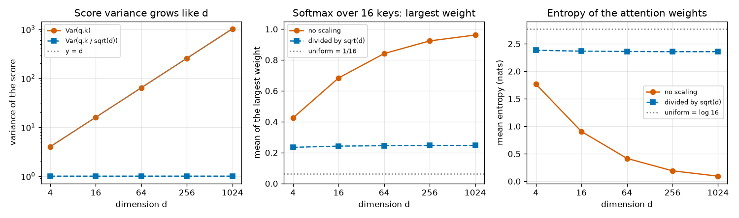
The last two lines of output are the gradients 0.00034 and 0.19661 computed by hand above. Three things can be read from the figure and the rest of the output.
- Left: the variance of the undivided scores overlaps the dashed gray line \(y = d\) (4.00, 15.99, 64.05, 256.19, 1024.57), exactly the derived \(\operatorname{Var}(q\cdot k) = d_k\). After dividing, it is 1 regardless of dimension.
- Middle: without division, one key monopolizes the weight more and more as the dimension grows: 0.842 on average at \(d = 64\) and 0.962 at \(d = 1024\). Even though these are random vectors that have learned nothing, attention starts out “looking at only one place”. With division, it stays around 0.25 at every dimension.
- Right: the entropy tells the same story. Without division it drops to 0.093 at \(d = 1024\); with division it stays around 2.36 (slightly below the fully uniform 2.773, because score differences with variance 1 still make the weights differ somewhat).
Scope of the assumption
The assumption “independent components with variance 1” describes the start of training. As training progresses, the model can grow its weights and produce attention as sharp as it needs (the experiment at the end of this chapter shows weight concentrating almost entirely on one shape). Dividing by \(\sqrt{d_k}\) is not a device to prevent sharp attention; it places the starting point where gradients flow well. Also note that the original paper did not prove this explanation experimentally; it wrote that it “suspects” this is the case.
Self-attention and cross-attention
So far, queries, keys, and values have been “given”. In practice they are made from tokens. Attention gets one of two names depending on which set of tokens they are made from.
- Self-attention: queries, keys, and values all come from the same set of tokens \(X\). The tokens look at each other. \(N_q = N_k = N\); \(N\) tokens go in and \(N\) come out.
- Cross-attention: queries come from one set \(Z\), and keys and values from another set \(M\). The tokens of \(Z\) look at the tokens of \(M\) and fetch information. If \(Z\) has \(N_q\) tokens, so does the output. \(M\) is unchanged.
“Made from tokens” means multiplied by learned matrices. With matrices \(W_Q, W_K \in \mathbb{R}^{D \times d_k}\) and \(W_V \in \mathbb{R}^{D \times d_v}\):
\(\begin{aligned} \text{자기 어텐션:}\quad & Q = X W_Q, \quad K = X W_K, \quad V = X W_V \\ \text{교차 어텐션:}\quad & Q = Z W_Q, \quad K = M W_K, \quad V = M W_V \end{aligned}\)
The operation itself is the same \(\operatorname{softmax}(QK^\top/\sqrt{d_k})\,V\); only the source of the ingredients differs. In this tutorial, the two kinds of attention appear in the following places.
| Where | Type | Source of queries | Source of keys and values | Details |
| Backbone (ViT) | Self-attention | Image tokens | The same image tokens | |
| Decoder | Self-attention | Object queries | The same object queries | |
| Decoder | Cross-attention | Object queries | Image tokens |
The heart of DETR-family detectors is the third row. Each object query scans all the image tokens and pulls in information from where its object is. That is also where the name “object query” comes from: these are the tokens placed in the query slot of cross-attention.
Figure 5-4 in the original depicts cross-attention in the DETR decoder. The 3 object queries on the left are the source of the queries \(Q\), and the 24 image tokens on the right (a grid) are the source of the keys \(K\) and values \(V\). The weights have shape (3, 24), so each query has one set of weights over all image tokens (the colored cells in the grid are the image tokens to which object query 1 gave large weights). The result is 3 new object queries of shape \((3, D)\); the number of outputs equals the number of queries.
Cost: the square of the token count
“Every token looks at every token” comes at a price. The score matrix \(S\) of self-attention is \(N \times N\), and each entry is a dot product of length \(d_k\). So the number of multiplications is roughly \(N^2 \cdot d_k\), and the memory for the weight matrix is also proportional to \(N^2\). Table 1 of the original paper states this as a “complexity per layer of \(O(N^2 \cdot D)\)”. \(O(\cdot)\) is notation meaning “grows at this rate, ignoring constant factors”.
For images, the token count is (side length in pixels ÷ patch size)². Halving the patch size or doubling the resolution multiplies the tokens by 4 and the token pairs by 16.
| Image side | Patch size | Grid | Tokens \(N\) | Token pairs \(N^2\) | Relative to patch 16 |
| 96 | 16 | 6×6 | 36 | 1,296 | 1× |
| 96 | 8 | 12×12 | 144 | 20,736 | 16× |
| 96 | 4 | 24×24 | 576 | 331,776 | 256× |
| 96 | 2 | 48×48 | 2,304 | 5,308,416 | 4,096× |
The shapes world is a toy, but real models follow the same arithmetic. Counting patch tokens for the configurations in Table 7 of the RF-DETR paper gives the following (excluding the few special tokens the backbone adds; see chapter 6).
| Model (paper Table 7) | Resolution | Patch size | Grid | Tokens \(N\) | Token pairs \(N^2\) |
| RF-DETR N | 384 | 16 | 24×24 | 576 | 331,776 |
| RF-DETR M | 576 | 16 | 36×36 | 1,296 | 1,679,616 |
| RF-DETR 2XL | 880 | 20 | 44×44 | 1,936 | 3,748,096 |
Going from N to 2XL multiplies the tokens by 3.4 but the token pairs by 11.3. For a real-time detector this quadratic cost is a heavy burden, and two later chapters are about lightening exactly this burden.
- Deformable attention in chapter 8: in the decoder's cross-attention, each query looks at only a few points instead of all image tokens.
- Window attention in chapter 9: in the backbone's self-attention, the image is split into a few windows and only tokens in the same window look at each other. With 4 windows, the number of pairs drops to \(4 \times (N/4)^2 = N^2/4\).
At the end of this chapter, we measure actual time while increasing the token count.
Masks: hiding what must not be seen
Sometimes a query must be prevented from looking at a key at all. The way to do this is to add \(-\infty\) to that score before the softmax. Build a matrix \(M^{\text{mask}} \in \mathbb{R}^{N_q \times N_k}\) that is \(-\infty\) at blocked positions and 0 elsewhere, and add it to the scores.
\(A = \operatorname{softmax}\!\left( \frac{QK^\top}{\sqrt{d_k}} + M^{\text{mask}} \right), \qquad M^{\text{mask}}_{ij} = \begin{cases} -\infty & (i, j)\text{ 를 막을 때} \\ 0 & \text{그 밖} \end{cases}\)
- Adding −∞ makes the weight exactly 0
- \(\exp(s_j + (-\infty)) = \exp(-\infty) = 0\)
- The exponential function \(e^x\) approaches 0 as \(x\) decreases, and its limit as \(x \to -\infty\) is 0. At blocked positions, the softmax numerator becomes 0.
- The numerator is 0, so the weight is 0. Not a tiny value but exactly 0, so that value vector does not mix into the output at all.
- The blocked terms drop out of the denominator. This is the same as taking the softmax over the remaining keys only, so the weights still sum to 1.
Let us mask the third key in the worked example. The first query's scores were \((2.8284, 0, 1.4142)\). Removing the third gives \(e^{2.8284} + e^{0} = 16.919 + 1 = 17.919\), and the weights are \((16.919/17.919,\; 1/17.919,\; 0) = (0.9442,\; 0.0558,\; 0)\). The 0.1867 that used to go to the third token has been redistributed proportionally to the other two.
Masks go by two names depending on their use, and PyTorch argument names follow the same naming.
- Key padding mask, shape
(B, N_k): to batch images of different sizes together, smaller images must be filled with empty cells (padding) to match sizes. The padded fake tokens are hidden entirely on the key side so that no query can see them. Since each image has different positions to hide, there is a batch axis. - Attention mask, shape
(N_q, N_k): decides visibility for each (query, key) pair. You can freely specify “query \(i\) cannot see key \(j\)”.
The attention mask appears again later. LW-DETR and RF-DETR use a technique called Group DETR, which splits object queries into several groups during training (chapter 9, chapter 11), and in the decoder's self-attention, queries in different groups must not see each other. A single attention mask that “blocks if the groups differ” implements this. (RF-DETR's public code achieves the same effect differently: instead of a mask, it slices the queries by group and runs self-attention on each group separately.) The second example in the code below is a miniature of this, with 4 queries split into two groups.
def mask_examples(x):
    """마스크 두 가지. True = 막는다."""
    # (1) 열쇠 패딩 마스크: 세 번째 토큰이 '채우기용 빈 토큰' 이라고 하자 → 모든 질의가 그 열쇠를 못 본다.
    key_padding = torch.tensor([False, False, True])  # (N_k,)
    _, w_pad = scaled_dot_product_attention(x, x, x, mask=key_padding[None, :])  # (1, N_k) → (N_q, N_k) 로 넓혀짐
    print("[마스크] 세 번째 열쇠를 가린 가중치 =\n", w_pad)

    # (2) 어텐션 마스크: 질의 4개를 두 묶음 {0, 1}, {2, 3} 으로 나누고, 다른 묶음은 서로 못 보게 한다.
    group = torch.tensor([0, 0, 1, 1])
    attn_mask = group[:, None] != group[None, :]  # (4, 4): 묶음이 다르면 True
    tokens = torch.randn(4, 8, generator=torch.Generator().manual_seed(0))
    _, w_group = scaled_dot_product_attention(tokens, tokens, tokens, mask=attn_mask)
    print("[마스크] 묶음 마스크 =\n", attn_mask.int())
    print("[마스크] 묶음끼리만 보는 가중치 =\n", w_group)
[마스크] 세 번째 열쇠를 가린 가중치 =
 tensor([[0.9442, 0.0558, 0.0000],
        [0.0558, 0.9442, 0.0000],
        [0.5000, 0.5000, 0.0000]])
[마스크] 묶음 마스크 =
 tensor([[0, 0, 1, 1],
        [0, 0, 1, 1],
        [1, 1, 0, 0],
        [1, 1, 0, 0]], dtype=torch.int32)
[마스크] 묶음끼리만 보는 가중치 =
 tensor([[0.9122, 0.0878, 0.0000, 0.0000],
        [0.2729, 0.7271, 0.0000, 0.0000],
        [0.0000, 0.0000, 0.9958, 0.0042],
        [0.0000, 0.0000, 0.0237, 0.9763]])
The first row of the first output is the \((0.9442, 0.0558, 0)\) just computed by hand. In the second output, weights remain only in the top-left 2×2 and bottom-right 2×2 blocks: groups \(\{0, 1\}\) and \(\{2, 3\}\) are completely cut off from each other.
Blocking an entire row gives NaN
If a query cannot see any key, the softmax becomes \(0/0\), producing NaN (not a number), which then spreads all the way to the loss. When building a mask, make sure every query can see at least one key. If the loss suddenly becomes NaN during training, this is one place to look.
Multi-head attention
Why multiple heads
A single attention step produces only one set of weights per query. But a token may want to know several things. An image token on the edge of a shape might want to know both “how far do the tokens of my color extend?” and “what is right next to me?”. Trying to see both with one set of weights averages them into a blur. In the original paper's words, “with a single attention head, averaging inhibits this”.
Multi-head attention runs \(h\) small attentions side by side. Each is called a head. Each head makes its own queries, keys, and values with its own projection matrices, so different heads can look at different places by different criteria. At the end, the heads' outputs are concatenated.
Four projection matrices and shape tracking
Head \(i\) (\(i = 1, \dots, h\)) has projection matrices \(W_i^Q, W_i^K \in \mathbb{R}^{D \times d_k}\) and \(W_i^V \in \mathbb{R}^{D \times d_v}\). With the query source \(X_q \in \mathbb{R}^{N_q \times D}\) and the key-value source \(X_k \in \mathbb{R}^{N_k \times D}\) (identical for self-attention):
\(\begin{aligned} \text{head}_i &= \operatorname{Attention}\big(X_q W_i^Q,\; X_k W_i^K,\; X_k W_i^V\big) \in \mathbb{R}^{N_q \times d_v} \\ \operatorname{MultiHead}(X_q, X_k) &= \operatorname{Concat}(\text{head}_1, \dots, \text{head}_h)\, W^O \in \mathbb{R}^{N_q \times D} \end{aligned}\)
\(\operatorname{Concat}\) joins the outputs of the \(h\) heads side by side into \((N_q, h\, d_v)\), and \(W^O \in \mathbb{R}^{h d_v \times D}\) is the output projection that mixes the concatenation back down to \(D\) dimensions. The head dimension is usually set to \(D\) divided by the number of heads.
\(d_k = d_v = \frac{D}{h}\)
The original paper uses \(D = 512\) and \(h = 8\), so \(d_k = 64\). The decoder in RF-DETR's default configuration has \(D = 256\) and 8 self-attention heads, so \(d_k = 256/8 = 32\). Splitting this way keeps the total cost of many heads about the same as “one head of dimension \(D\)”: one head does \(N_q N_k\, d_k\) multiplications, so \(h\) heads do \(h \cdot N_q N_k \cdot (D/h) = N_q N_k D\).
Implementations do not keep a separate small matrix per head. Concatenating \(W_1^Q, \dots, W_h^Q\) side by side gives a single \(D \times (h\,d_k) = D \times D\) matrix \(W_Q\), so you compute \(X W_Q\) once and then split the \(D\) columns of the result into \(h\) groups of \(d_k\) to get the per-head queries. The same goes for \(W_K\) and \(W_V\). So the parameters are just four \(D \times D\) matrices, \(W_Q, W_K, W_V, W_O\) (plus biases).
Figure 5-5 in the original shows the flow of multi-head self-attention. Tokens \((N, D)\) pass through the linear projections \(W_Q, W_K, W_V\) and are split into \(h\) heads; heads 1, 2, …, \(h\) each attend separately at size \((N, D/h)\). Concatenating the heads' outputs gives \((N, D)\) again, which \(W_O\) mixes before output. The shape that comes out is the same \((N, D)\) that went in.
Following the tensor shapes with the batch included gives the table below. Match it line by line with the code.
| Step | Operation | Shape | \(B = 2\), \(N_q = 5\), \(N_k = 12\), \(D = 256\), \(h = 8\) |
| Input | Query source / key-value source | \((B, N_q, D)\) / \((B, N_k, D)\) | (2, 5, 256) / (2, 12, 256) |
| Projection | Multiply by \(W_Q\), \(W_K\), \(W_V\) | Unchanged | (2, 5, 256) / (2, 12, 256) |
| Split into heads | Last axis into \((h, d_k)\), head axis moved forward | \((B, h, N_q, d_k)\) / \((B, h, N_k, d_k)\) | (2, 8, 5, 32) / (2, 8, 12, 32) |
| Scores, weights | \(QK^\top/\sqrt{d_k}\), softmax | \((B, h, N_q, N_k)\) | (2, 8, 5, 12) |
| Per-head output | \(AV\) | \((B, h, N_q, d_k)\) | (2, 8, 5, 32) |
| Concatenate | Move the head axis back and merge | \((B, N_q, h\,d_k) = (B, N_q, D)\) | (2, 5, 256) |
| Output projection | Multiply by \(W_O\) | \((B, N_q, D)\) | (2, 5, 256) |
Counting parameters
Let us count the parameters of multi-head attention with \(D = 256\) and \(h = 8\) by hand. A PyTorch linear layer has a bias vector in addition to its weight matrix.
- 263,168 parameters for D = 256
- \(W_Q:\quad D \times D + D = 256 \times 256 + 256 = 65{,}536 + 256 = 65{,}792\)
- \(D \times D\) weights and \(D\) biases. The \(256 \times 256\) matrix is the eight heads' \(256 \times 32\) matrices concatenated.
- All four projections are \(D \to D\) linear layers, so they are the same size.
- The number of heads \(h\) does not appear in the formula. Whether there is 1 head or 8, the parameter count is the same; the only difference is “how many groups those parameters are split into”.
Implementation and comparison with the built-in module
Now we implement it. All it takes is adding the four projections and “split into heads, concatenate” to the scaled_dot_product_attention built earlier. The two masks are combined into a form that broadcasts to (B, 1, N_q, N_k) (the 1 in the middle is the head axis: the same mask for every head).
class MultiHeadAttention(nn.Module):
    """다중 머리 어텐션. 입력 · 출력 모두 (B, N, D) — 배치가 맨 앞이다.

    D 차원을 머리 h 개로 나눠(머리마다 d_k = D / h 차원) 머리마다 따로 어텐션한 뒤 다시 이어 붙인다.
    매개변수는 투영 넷(W_Q, W_K, W_V, W_O)뿐이고, 저마다 D × D 가중치와 길이 D 의 편향을 가진다.
    """

    def __init__(self, dim: int, num_heads: int):
        super().__init__()
        assert dim % num_heads == 0, "dim 은 머리 수로 나누어떨어져야 한다"
        self.dim, self.num_heads, self.head_dim = dim, num_heads, dim // num_heads
        self.q_proj = nn.Linear(dim, dim)  # W_Q: 머리 h 개의 (D → d_k) 투영을 한 행렬에 쌓은 것
        self.k_proj = nn.Linear(dim, dim)  # W_K
        self.v_proj = nn.Linear(dim, dim)  # W_V
        self.out_proj = nn.Linear(dim, dim)  # W_O: 이어 붙인 머리들을 다시 섞는다

    def split_heads(self, x):
        """(B, N, D) → (B, h, N, d_k). 마지막 축 D 를 (h, d_k) 로 쪼개고 머리 축을 앞으로 보낸다."""
        b, n, _ = x.shape
        return x.view(b, n, self.num_heads, self.head_dim).transpose(1, 2)

    def forward(self, query, key, value, key_padding_mask=None, attn_mask=None):
        """query (B, N_q, D), key · value (B, N_k, D).

        key_padding_mask: (B, N_k) bool — True 인 열쇠는 아무도 보지 못한다(그림마다 다른 패딩).
        attn_mask: (N_q, N_k) bool — True 인 (질의, 열쇠) 쌍을 막는다(모든 그림 · 모든 머리에 공통).
        돌려주는 값: 출력 (B, N_q, D), 머리별 가중치 (B, h, N_q, N_k).
        """
        b, n_q, _ = query.shape
        q = self.split_heads(self.q_proj(query))  # (B, h, N_q, d_k)
        k = self.split_heads(self.k_proj(key))  # (B, h, N_k, d_k)
        v = self.split_heads(self.v_proj(value))  # (B, h, N_k, d_k)

        mask = None  # 두 마스크를 (B, 1, N_q, N_k) 로 넓혀질 수 있는 하나로 합친다
        if key_padding_mask is not None:
            mask = key_padding_mask[:, None, None, :]  # (B, 1, 1, N_k)
        if attn_mask is not None:
            mask = attn_mask[None, None] if mask is None else mask | attn_mask[None, None]

        out, weights = scaled_dot_product_attention(q, k, v, mask)  # (B, h, N_q, d_k), (B, h, N_q, N_k)
        out = out.transpose(1, 2).reshape(b, n_q, self.dim)  # 머리들을 이어 붙인다: (B, N_q, h·d_k = D)
        return self.out_proj(out), weights
To confirm it is correct, compare it with PyTorch's built-in nn.MultiheadAttention. The built-in module stores \(W_Q, W_K, W_V\) stacked vertically as a single in_proj_weight, so we just concatenate our weights in that order and copy them in. The same input should give the same output.
def copy_to_builtin(mine: MultiHeadAttention) -> nn.MultiheadAttention:
    """직접 만든 다중 머리 어텐션의 가중치를 PyTorch 내장 nn.MultiheadAttention 에 옮긴다.

    내장 모듈은 W_Q, W_K, W_V 를 세로로 쌓은 in_proj_weight (3D, D) 한 덩어리로 갖고 있다.
    """
    builtin = nn.MultiheadAttention(mine.dim, mine.num_heads, batch_first=True)
    with torch.no_grad():
        builtin.in_proj_weight.copy_(torch.cat([mine.q_proj.weight, mine.k_proj.weight, mine.v_proj.weight]))
        builtin.in_proj_bias.copy_(torch.cat([mine.q_proj.bias, mine.k_proj.bias, mine.v_proj.bias]))
        builtin.out_proj.weight.copy_(mine.out_proj.weight)
        builtin.out_proj.bias.copy_(mine.out_proj.bias)
    return builtin

def check_multi_head(seed=0):
    """d = 256, h = 8 에서 매개변수 수를 세고, 내장 모듈과 출력 · 가중치를 비교한다."""
    torch.manual_seed(seed)
    dim, heads = 256, 8
    mine = MultiHeadAttention(dim, heads).eval()
    builtin = copy_to_builtin(mine).eval()
    count = sum(p.numel() for p in mine.parameters())
    print(f"[다중 머리] 매개변수 수: 직접 구현 {count:,}, 내장 {sum(p.numel() for p in builtin.parameters()):,}"
          f" (손계산 4 × (256·256 + 256) = {4 * (256 * 256 + 256):,})")

    query = torch.randn(2, 5, dim)  # 질의 5개 (예: 객체 질의)
    memory = torch.randn(2, 12, dim)  # 열쇠 · 값 12개 (예: 그림 토큰)
    key_padding = torch.zeros(2, 12, dtype=torch.bool)
    key_padding[1, 9:] = True  # 둘째 그림의 마지막 토큰 3개는 패딩
    with torch.no_grad():
        out, weights = mine(query, memory, memory, key_padding_mask=key_padding)
        ref_out, ref_weights = builtin(query, memory, memory, key_padding_mask=key_padding,
                                       need_weights=True, average_attn_weights=False)
        print(f"[다중 머리] 교차 어텐션 모양: 출력 {tuple(out.shape)}, 가중치 {tuple(weights.shape)}")
        print(f"[check] nn.MultiheadAttention 과의 최대 차이: 출력 {(out - ref_out).abs().max().item():.2e},"
              f" 가중치 {(weights - ref_weights).abs().max().item():.2e}")
        print(f"[check] 패딩된 열쇠의 가중치 합: {weights[1, :, :, 9:].sum().item():.1f},"
              f" 가중치 행의 합(모두 1 이어야): 최소 {weights.sum(-1).min().item():.6f} 최대 {weights.sum(-1).max().item():.6f}")

        # 자기 어텐션 + 어텐션 마스크(질의 묶음 둘)도 대조한다
        x = torch.randn(2, 6, dim)
        group = torch.tensor([0, 0, 0, 1, 1, 1])
        attn_mask = group[:, None] != group[None, :]
        out2, _ = mine(x, x, x, attn_mask=attn_mask)
        ref2, _ = builtin(x, x, x, attn_mask=attn_mask, need_weights=False)
        print(f"[check] 어텐션 마스크를 준 자기 어텐션의 최대 차이: {(out2 - ref2).abs().max().item():.2e}")

        # F.scaled_dot_product_attention 과도 같은지 (머리 하나짜리로)
        q, k, v = torch.randn(3, 7, 32), torch.randn(3, 9, 32), torch.randn(3, 9, 32)
        ours, _ = scaled_dot_product_attention(q, k, v)
        print(f"[check] F.scaled_dot_product_attention 과의 최대 차이:"
              f" {(ours - F.scaled_dot_product_attention(q, k, v)).abs().max().item():.2e}")
    return mine
[다중 머리] 매개변수 수: 직접 구현 263,168, 내장 263,168 (손계산 4 × (256·256 + 256) = 263,168)
[다중 머리] 교차 어텐션 모양: 출력 (2, 5, 256), 가중치 (2, 8, 5, 12)
[check] nn.MultiheadAttention 과의 최대 차이: 출력 1.19e-07, 가중치 4.47e-08
[check] 패딩된 열쇠의 가중치 합: 0.0, 가중치 행의 합(모두 1 이어야): 최소 1.000000 최대 1.000000
[check] 어텐션 마스크를 준 자기 어텐션의 최대 차이: 1.79e-07
[check] F.scaled_dot_product_attention 과의 최대 차이: 4.77e-07
- The parameter count matches the hand-computed 263,168 and also the built-in module.
- In cross-attention between 5 queries and 12 image tokens, the output is (2, 5, 256) and the weights are (2, 8, 5, 12), exactly the shapes in the table above.
- The difference from the built-in module is on the order of \(10^{-7}\). That is the size of 32-bit floating-point rounding error, so the two can be regarded as the same computation. The same holds with a key padding mask and with an attention mask.
- The weights on the 3 padded keys sum to exactly 0.0, and every row of weights sums to 1.
RF-DETR's public code also uses the built-in nn.MultiheadAttention for the decoder's self-attention. Since we have confirmed here that the two compute the same thing, whenever you meet the built-in module in later chapters, you can think of the code in this section.
Attention does not know order
Permutation equivariance
Look at the attention formula again: “which position is this token in” appears nowhere. Scores are just dot products between contents. So if you feed the tokens in shuffled order, the output comes out shuffled the same way, with the values themselves unchanged. This property is called permutation equivariance. Here it is in equations.
Reordering tokens is written as multiplying by a permutation matrix \(P\). \(P\) is an \(N \times N\) matrix with exactly one 1 in each row and each column and 0 elsewhere. \(PX\) rearranges the rows (tokens) of \(X\), and multiplying by \(P^\top\) on the right rearranges the columns in the same order. Shuffling and then unshuffling restores the original, so \(P^\top P = I\) (the identity matrix).
- Feeding shuffled tokens PX into self-attention gives P·(original output)
- \(Q' = (PX) W_Q = P (X W_Q) = P Q, \qquad K' = P K, \qquad V' = P V\)
- Matrix multiplication can be regrouped (associativity). The projection is computed per token, so shuffling then projecting equals projecting then shuffling.
- \((PK)^\top = K^\top P^\top\). The score table only has its rows (queries) and columns (keys) rearranged in the same order; the numbers inside are unchanged.
- Softmax is computed row by row, and within a row each number's result is the same no matter how the numbers are ordered. So the rearranging of rows and columns can be swapped with the softmax.
- \(P^\top P = I\) vanishes in the middle. The output \(O'\) for the shuffled input is the original output \(O\) shuffled in the same order.
Checking with the worked example: feeding the tokens in the order \((x_2, x_1, x_3)\), the output for \(x_1 = (2, 0)\) is still \((1.7225, 0.2775)\). It just appears in the second slot instead of the first. This property holds even when many layers are stacked and when the FFN and layer normalization described later are inserted (all of them are computed per token).
For images this is fatal. If each token's output stays the same even when the 144 image tokens are shuffled at random, the model has no way of knowing where in the image the red patch is. For a detector that must predict box coordinates, position is everything. The DETR paper also writes that “since the transformer architecture is permutation-invariant, we supplement it with fixed positional encodings”.
Equivariant vs. invariant
If shuffling the input shuffles the output along with it, the function is equivariant (\(f(PX) = P f(X)\)); if shuffling the input leaves the output entirely unchanged, it is invariant (\(f(PX) = f(X)\)). A self-attention layer itself is equivariant, and averaging its output over the tokens (an order-independent operation) makes it invariant. Papers sometimes lump the two together as “permutation invariant”.
def check_permutation(mine: MultiHeadAttention, seed=0):
    """자기 어텐션은 토큰을 섞어 넣으면 출력도 똑같이 섞여 나올 뿐이다(순열 등변성)."""
    gen = torch.Generator().manual_seed(seed)
    x = torch.randn(1, 10, mine.dim, generator=gen)  # 토큰 10개
    perm = torch.randperm(10, generator=gen)  # 섞는 순서
    with torch.no_grad():
        out, _ = mine(x, x, x)
        out_perm, _ = mine(x[:, perm], x[:, perm], x[:, perm])  # 섞어서 넣기
        diff = (out_perm - out[:, perm]).abs().max().item()  # "섞어 넣은 출력" 과 "출력을 섞은 것" 의 차이
        pos = sine_position_1d(10, mine.dim)[None]  # 위치 인코딩을 더하면?
        out_pos, _ = mine(x + pos, x + pos, x + pos)
        out_pos_perm, _ = mine(x[:, perm] + pos, x[:, perm] + pos, x[:, perm] + pos)
        diff_pos = (out_pos_perm - out_pos[:, perm]).abs().max().item()
    print(f"[순열] 섞는 순서 {perm.tolist()}")
    print(f"[순열] 위치 인코딩 없음: |f(PX) − P f(X)| 의 최댓값 = {diff:.2e}  (0 → 순서를 모른다)")
    print(f"[순열] 위치 인코딩 더함: 같은 차이 = {diff_pos:.3f}  (0 이 아님 → 순서가 출력을 바꾼다)")
[순열] 섞는 순서 [6, 9, 0, 2, 4, 8, 1, 5, 3, 7]
[순열] 위치 인코딩 없음: |f(PX) − P f(X)| 의 최댓값 = 1.19e-07  (0 → 순서를 모른다)
[순열] 위치 인코딩 더함: 같은 차이 = 0.150  (0 이 아님 → 순서가 출력을 바꾼다)
The difference between the output for 10 shuffled tokens and the original output shuffled in the same order is \(1.19 \times 10^{-7}\) (rounding error). As derived, attention does not know order. The second line adds the positional encoding, explained next, to the tokens. The same difference is now 0.150: “which position a token is in” now changes the output.
Sinusoidal positional encoding
The solution is to add the information “I am at position so-and-so” directly to each token. A different vector is made for each position and added to the token vector. This vector is called a positional encoding. Since it is added to the token, it has the same dimension \(D\). The original paper uses fixed, non-learned vectors built from sine and cosine functions. In the encoding for position \(pos\) (\(0, 1, 2, \dots\)), the components come in pairs.
\(\begin{aligned} PE(pos,\, 2i) &= \sin\!\big(pos \cdot \omega_i\big), \\ PE(pos,\, 2i+1) &= \cos\!\big(pos \cdot \omega_i\big), \end{aligned} \qquad \omega_i = \frac{1}{10000^{\,2i/D}}, \qquad i = 0, 1, \dots, \tfrac{D}{2} - 1\)
\(PE(pos, c)\) is component \(c\) of the encoding vector for position \(pos\). \(\omega_i\) (omega) is the angular frequency of pair \(i\), which sets how far the sine's angle turns when the position increases by 1. The original paper writes \(\sin(pos / 10000^{2i/D})\), which is the same formula. At \(i = 0\), \(\omega_0 = 1\) turns fastest, and it slows as \(i\) grows. The number of positions for one full turn (the wavelength) is \(2\pi/\omega_i = 2\pi \cdot 10000^{2i/D}\), so the fastest pair has wavelength \(2\pi \approx 6.28\) and the slowest approaches \(10000 \cdot 2\pi\).
Let us compute the smallest example, \(D = 4\), by hand. There are two pairs, with \(\omega_0 = 1/10000^{0} = 1\) and \(\omega_1 = 1/10000^{2/4} = 1/100 = 0.01\).
| \(pos\) | \(\sin(pos \cdot 1)\) | \(\cos(pos \cdot 1)\) | \(\sin(pos \cdot 0.01)\) | \(\cos(pos \cdot 0.01)\) |
| 0 | 0.0000 | 1.0000 | 0.0000 | 1.0000 |
| 1 | 0.8415 | 0.5403 | 0.0100 | 0.9999 |
| 2 | 0.9093 | −0.4161 | 0.0200 | 0.9998 |
| 3 | 0.1411 | −0.9900 | 0.0300 | 0.9996 |
Angles are in radians (\(\sin 1 = 0.8415\)). The first two components change a lot from position to position, while the last two change very slowly. In code, a single sine_embed that takes real-valued positions is written once, and the 1D and 2D encodings call it.
def sine_embed(position, dim: int, temperature: float = 10000.0):
    """실수 위치(임의 모양 (...))를 사인 · 코사인 dim 개로 바꾼다 → (..., dim).

    짝수 번째 성분 2i 는 sin(위치 · ω_i), 홀수 번째 성분 2i+1 은 cos(위치 · ω_i),
    각진동수 ω_i = 1 / temperature^(2i / dim)  (i = 0, 1, …, dim/2 − 1).
    """
    assert dim % 2 == 0
    i = torch.arange(dim // 2, dtype=torch.float32)
    omega = 1.0 / temperature ** (2 * i / dim)  # (dim/2,): 1 에서 시작해 점점 느려지는 각진동수
    angle = position[..., None].float() * omega  # (..., dim/2)
    return torch.stack([angle.sin(), angle.cos()], dim=-1).flatten(-2)  # sin, cos 를 번갈아 놓는다

def sine_position_1d(length: int, dim: int, temperature: float = 10000.0):
    """원 논문("Attention Is All You Need" 3.5절)의 위치 인코딩. 위치 0, 1, …, length−1 → (length, dim)."""
    return sine_embed(torch.arange(length), dim, temperature)
[위치] sine_position_1d(4, 4) =
 tensor([[ 0.0000,  1.0000,  0.0000,  1.0000],
        [ 0.8415,  0.5403,  0.0100,  0.9999],
        [ 0.9093, -0.4161,  0.0200,  0.9998],
        [ 0.1411, -0.9900,  0.0300,  0.9996]])
[위치] d = 64: PE(32)·PE(32) = 32.00, PE(32)·PE(33) = 30.92, PE(32)·PE(36) = 23.93, PE(32)·PE(48) = 19.37
[위치] 위치가 달라도 간격이 같으면 내적이 같다: PE(10)·PE(14) = 23.93, PE(50)·PE(54) = 23.93
[위치] sine_position_2d(12, 12, 64) 모양 (144, 64), 같은 행의 두 토큰은 앞 절반(y)이 같다: True, 같은 열의 두 토큰은 뒤 절반(x)이 같다: True
The first table matches the hand computation above. The remaining lines are discussed shortly.
Why multiple frequencies
Think of a clock. The second hand turns fast, so it distinguishes even a one-second difference, but it returns to the same spot every minute. The hour hand never returns to the same spot within 12 hours, but it barely moves in a second. Only by reading both do you get a time that is “both precise and unambiguous”.
Positional encoding works the same way. Fast components (small \(i\)) clearly distinguish neighboring positions but return to the same values every 6 positions or so. Slow components (large \(i\)) distinguish distant positions but are nearly identical for neighbors. Placing many components side by side, from fast to slow, gives every position a different vector while keeping nearby positions' vectors similar.
“Near means similar” can be stated precisely with the dot product. This is where the reason for putting sine and cosine in pairs becomes clear.
- The dot product of two positional encodings depends only on the offset
- \(PE(p) \cdot PE(p + \Delta) = \sum_{i=0}^{D/2 - 1} \Big[ \sin(\omega_i p)\,\sin\!\big(\omega_i (p + \Delta)\big) + \cos(\omega_i p)\,\cos\!\big(\omega_i (p + \Delta)\big) \Big]\)
- \(PE(p)\) is the whole encoding vector for position \(p\), and \(\Delta\) (delta) is the offset between the two positions. The dot product is written per pair (\(i\)), multiplying sine components together and cosine components together.
- This uses the trigonometric angle-difference identity \(\cos(\beta - \gamma) = \cos\beta\cos\gamma + \sin\beta\sin\gamma\) with \(\beta = \omega_i(p + \Delta)\) and \(\gamma = \omega_i p\).
- \(p\) has disappeared. The dot product depends only on the offset \(\Delta\), not on where the two positions are. At \(\Delta = 0\) there are \(D/2\) terms of \(\cos 0 = 1\), giving the maximum \(D/2\); as the offset grows, the cosines move away from 1, fast components first, and the dot product shrinks.
In the output above, this is the line starting with [위치] d = 64 and the line after it. At \(D = 64\), the dot product with itself is \(D/2 = 32.00\), and it drops to 30.92 one position away, 23.93 four positions away, and 19.37 sixteen positions away. Also, the dot product of positions 10 and 14 (23.93) equals that of positions 50 and 54 (23.93), because both offsets are 4.
- Figure: Figure 5-6 1D sinusoidal positional encoding (\(D = 64\), positions 0–63). Left: heatmap with positions as rows and components as columns (red +1, blue −1). Middle: waveforms of four components. Right: dot products of a reference position with every other position.
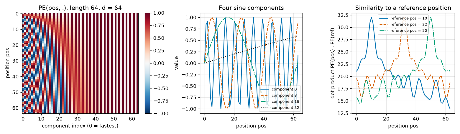
- Left: each row is the encoding vector of one position. The left columns (fast components) alternate red and blue frequently from top to bottom, while the right columns (slow components) barely change and look like vertical stripes (sine near 0, cosine near 1). No two rows are identical.
- Middle: component 0 has wavelength \(2\pi \approx 6.3\), component 8 (\(i = 4\)) \(2\pi \cdot 10000^{8/64} \approx 19.9\), component 16 (\(i = 8\)) \(2\pi \cdot 10 \approx 62.8\), and component 32 (\(i = 16\)) \(2\pi \cdot 100 \approx 628\). The last one is almost a straight line over this range.
- Right: the dot product is largest at the reference position (32) and decreases with distance. The three curves differ only in where their peaks are and have the same shape, exactly the “depends only on the offset” just derived.
Why the original paper chose sinusoids
The original paper explains its choice of the sinusoidal form by saying it “hypothesized it would allow the model to easily learn to attend by relative positions”, since the encoding of a position offset by \(\Delta\) can be written as a linear function of the original encoding. Indeed, using the angle-addition identity, for one pair
\(\begin{pmatrix} \sin\omega_i(p + \Delta) \\ \cos\omega_i(p + \Delta) \end{pmatrix} = \begin{pmatrix} \cos\omega_i\Delta & \sin\omega_i\Delta \\ -\sin\omega_i\Delta & \cos\omega_i\Delta \end{pmatrix} \begin{pmatrix} \sin\omega_i p \\ \cos\omega_i p \end{pmatrix}\)
and the middle matrix is determined by \(\Delta\) alone, independent of \(p\). The same paper also tried learning a vector for each position and reports nearly identical results (row (E) of Table 3 in the paper). This tutorial calls the learned kind a “position embedding”; it is what ViT and DINOv2 use, so it is covered in chapter 6.
2D positional encoding for images
The position of an image token is not one number but two: (row, column). DETR extends the 1D encoding as follows: half of the \(D\) dimensions hold the sinusoidal encoding of the vertical coordinate \(y\), and the other half that of the horizontal coordinate \(x\).
\(PE_{2D}(x, y) = \big[\; \underbrace{PE_{D/2}(\tilde{y})}_{D/2\text{ 개}} \;,\; \underbrace{PE_{D/2}(\tilde{x})}_{D/2\text{ 개}} \;\big], \qquad \tilde{y} = 2\pi\,\frac{y}{H}, \quad \tilde{x} = 2\pi\,\frac{x}{W}\)
\(H\) and \(W\) are the height and width of the token grid (12 and 12 in the shapes world), and \(y = 1, \dots, H\) and \(x = 1, \dots, W\) are row and column numbers counted from 1. \(PE_{D/2}\) is the 1D formula above with \(D/2\) in place of \(D\) (for \(D = 64\), 32 components per axis, 16 pairs, \(\omega_i = 10000^{-i/16}\)). \(\tilde{y}, \tilde{x}\) (tilde) are the coordinates rescaled to the range \((0, 2\pi]\). DETR's public code does this so that coordinates fall in the same range whether the grid is 12×12 or 40×40.
Let us check with numbers. The top row of a 12×12 grid (\(y = 1\)) has \(\tilde{y} = 2\pi/12 = 0.5236\), and its fastest component is \(\sin(0.5236 \cdot 1) = 0.5\). The third row (\(y = 3\)) has \(\tilde{y} = \pi/2\), so \(\sin(\pi/2) = 1\); the bottom row (\(y = 12\)) has \(\tilde{y} = 2\pi\), so \(\sin(2\pi) = 0\). The fastest component makes exactly one full turn from the top of the image to the bottom.
def sine_position_2d(height: int, width: int, dim: int, temperature: float = 10000.0, normalize: bool = True):
    """그림용 2차원 사인 위치 인코딩(DETR 방식) → (height · width, dim). 토큰 순서는 행 우선(위 줄부터 왼쪽 → 오른쪽).

    앞 절반 dim/2 개는 y(행) 좌표의 사인 인코딩, 뒤 절반 dim/2 개는 x(열) 좌표의 사인 인코딩이다.
    좌표는 1, 2, … 로 세고, normalize=True 면 (0, 2π] 범위로 바꾼다(격자 크기가 달라도 같은 범위를 쓰려고).
    """
    assert dim % 4 == 0
    y = torch.arange(1, height + 1, dtype=torch.float32)  # (H,)
    x = torch.arange(1, width + 1, dtype=torch.float32)  # (W,)
    if normalize:
        y, x = y / height * 2 * math.pi, x / width * 2 * math.pi
    pos_y = sine_embed(y, dim // 2, temperature)[:, None, :].expand(height, width, dim // 2)  # 같은 행은 같은 값
    pos_x = sine_embed(x, dim // 2, temperature)[None, :, :].expand(height, width, dim // 2)  # 같은 열은 같은 값
    return torch.cat([pos_y, pos_x], dim=-1).reshape(height * width, dim)
The last line of the output above checks the properties of this function. The shape is (144, 64); two tokens in the same row share the first half (\(y\)), and two tokens in the same column share the second half (\(x\)). This implementation was also separately checked against PositionEmbeddingSine(normalize=True) in RF-DETR's public code, with differences below \(10^{-6}\).
- Figure: Figure 5-7 2D sinusoidal positional encoding on a 12×12 grid (\(D = 64\)). Top row: four components drawn on the grid. Bottom row: dot products of the encoding at the reference position, marked with a red ×, with the encodings at every other position.
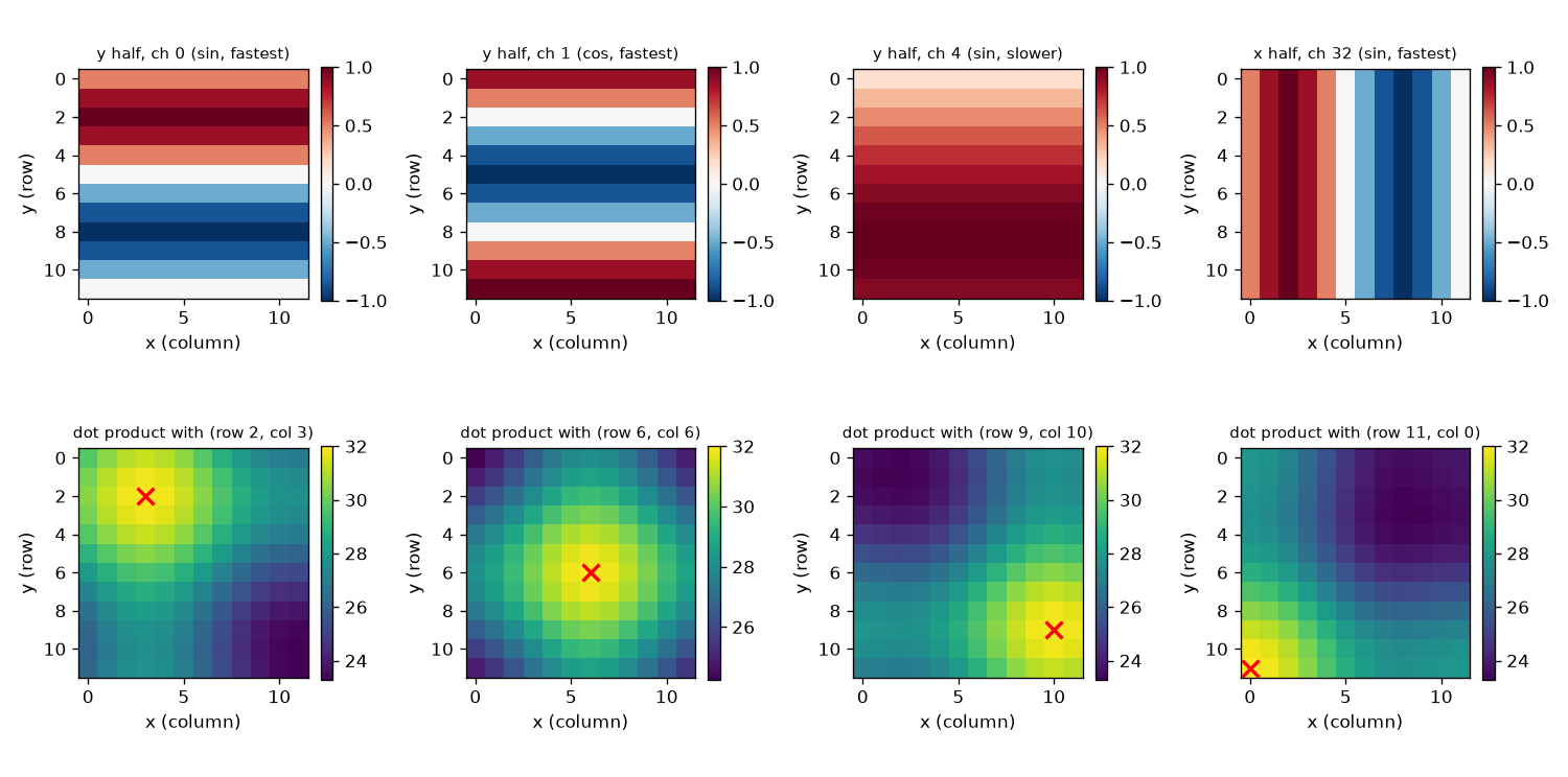
- Top row: the components of the \(y\) half (the left three) form horizontal stripes, because values are the same within a row. The first plot is the component just computed: 0.5 in the top row, 1 in the third row, 0 in the bottom row. The slow component (third plot) changes gradually from top to bottom. The component of the \(x\) half (fourth plot) forms vertical stripes.
- Bottom row: the dot product reaches its maximum \(D/2 = 32\) at the reference position and decreases with distance. This is because applying the 1D derivation to \(y\) and \(x\) separately gives a dot product of \(\sum_i \cos(\omega_i \Delta\tilde{y}) + \sum_i \cos(\omega_i \Delta\tilde{x})\). The dot product of positional encodings is itself a map of “how close things are in the image”.
Where the positional encoding is added varies by model. The original paper adds it once to the initial input tokens. DETR adds it to the queries and keys in every attention layer (the paper reports this worked best). See chapter 7 for details.
Assembling Transformer layers
The Transformer is the neural network architecture introduced in “Attention Is All You Need”: a stack of layers built around multi-head attention. The original paper was a translation model, with 6 encoder layers that read the sentence and 6 decoder layers that write the sentence. In a detector, the side that reads the image is the encoder (the backbone ViT in RF-DETR) and the side that outputs boxes is the decoder. Besides attention, three components are needed, two of which you already saw in chapter 4.
- Residual connection: add the input unchanged to a component's output (\(x + f(x)\)). It provides a shortcut for gradients.
- Layer normalization \(\operatorname{LN}\): normalizes the \(D\) components of a single token to mean 0 and variance 1, then applies a learned scale and shift.
- FFN: explained just below.
Thinking per token: the FFN
Attention only gathers information between tokens. Being a weighted average of values, it has little power to compute something new from the gathered information. So a small two-layer network is placed after attention. It is called an FFN (feed-forward network); many papers call it an MLP.
\(\operatorname{FFN}(x) = \max(0,\; x W_1 + b_1)\, W_2 + b_2, \qquad W_1 \in \mathbb{R}^{D \times rD}, \quad W_2 \in \mathbb{R}^{rD \times D}\)
\(x\) is one token (a row vector of length \(D\)), \(\max(0, \cdot)\) is ReLU, and \(b_1, b_2\) are biases. The hidden layer in the middle is \(r\) times wider than the token; \(r\) is called the expansion ratio. The original paper has \(D = 512\) with a hidden size of 2048, so \(r = 4\); RF-DETR's default decoder configuration has \(D = 256\) with a hidden size of 2048, so \(r = 8\). The key point is that the FFN is applied to each token separately, with the same weights. Only attention exchanges information between tokens; the FFN works within a single token.
The parameter count is \(D \cdot rD + rD\) for \(W_1\) and \(b_1\), and \(rD \cdot D + D\) for \(W_2\) and \(b_2\). With \(D = 256\) and \(r = 8\), that is \((256 \times 2048 + 2048) + (2048 \times 256 + 256) = 526{,}336 + 524{,}544 = 1{,}050{,}880\), about four times the attention (263,168). Most of a Transformer layer's parameters are in the FFN.
Encoder layer: post-norm and pre-norm
An encoder layer consists of two parts, “self-attention” and “FFN”, each wrapped in a residual connection and layer normalization. There are two schools of thought on the wrapping order. Writing the set of tokens as \(x\) and self-attention as \(\operatorname{SA}\):
\(\begin{aligned} \textbf{post-norm:}\quad & x' = \operatorname{LN}\big(x + \operatorname{SA}(x)\big), & y &= \operatorname{LN}\big(x' + \operatorname{FFN}(x')\big) \\ \textbf{pre-norm:}\quad & x' = x + \operatorname{SA}\big(\operatorname{LN}(x)\big), & y &= x' + \operatorname{FFN}\big(\operatorname{LN}(x')\big) \end{aligned}\)
- Post-norm (post-normalization): normalize after adding. This is what the original paper writes as “\(\operatorname{LayerNorm}(x + \operatorname{Sublayer}(x))\)”, and it is used by the DETR and RF-DETR decoders. The layer's output always comes out normalized.
- Pre-norm (pre-normalization): normalize before feeding into the component. ViT and DINOv2 use this. The formula has the form \(y = x + \operatorname{SA}(\cdot) + \operatorname{FFN}(\cdot)\), so the input \(x\) is added straight through to the output without ever passing through a normalization. Even in deep stacks, gradients flow directly along this shortcut. On the other hand, the output of the very last layer is left unnormalized, so ViT adds one more layer normalization at the very end of the stack.
In both styles the input and output have the same shape, (B, N, D), so the same layer can be stacked any number of times. The implementation supports both with one switch. If pos is given, the positional encoding is added only to the queries and keys, as in DETR.
class EncoderLayer(nn.Module):
    """Transformer 인코더 층: 자기 어텐션 + FFN. 두 부분 모두 잔차 연결과 층 정규화로 감싼다.

    pre_norm=False (post-norm, 원 논문 · DETR):  x ← LN(x + 부분층(x))
    pre_norm=True  (pre-norm, ViT · DINOv2):      x ← x + 부분층(LN(x))
    입력 · 출력 (B, N, D). pos 를 주면 DETR 처럼 질의 · 열쇠에만 더한다(값에는 더하지 않는다).
    """

    def __init__(self, dim: int, num_heads: int, ffn_ratio: int = 4, pre_norm: bool = False):
        super().__init__()
        self.pre_norm = pre_norm
        self.attn = MultiHeadAttention(dim, num_heads)
        self.norm1 = nn.LayerNorm(dim)
        self.ffn = nn.Sequential(  # 토큰마다 따로 적용되는 2층 신경망: D → ffn_ratio·D → D
            nn.Linear(dim, ffn_ratio * dim), nn.ReLU(), nn.Linear(ffn_ratio * dim, dim)
        )
        self.norm2 = nn.LayerNorm(dim)

    def self_attention(self, x, pos, key_padding_mask):
        qk = x if pos is None else x + pos  # 질의 = 열쇠 = (토큰 + 위치), 값 = 토큰
        return self.attn(qk, qk, x, key_padding_mask=key_padding_mask)[0]

    def forward(self, x, pos=None, key_padding_mask=None):
        if self.pre_norm:
            x = x + self.self_attention(self.norm1(x), pos, key_padding_mask)
            x = x + self.ffn(self.norm2(x))
        else:
            x = self.norm1(x + self.self_attention(x, pos, key_padding_mask))
            x = self.norm2(x + self.ffn(x))
        return x
[check] 인코더 층(post-norm) nn.TransformerEncoderLayer 와의 최대 차이: 7.15e-07
[check] 인코더 층(pre-norm ) nn.TransformerEncoderLayer 와의 최대 차이: 4.77e-07
[인코더 층] 매개변수 수 (D = 256, h = 8, FFN 2048): 어텐션 263,168, FFN 1,050,880, 층 정규화 2개 1,024 → 합 1,315,072
[인코더 층] 모양: 입력 (2, 20, 256) → 출력 (2, 20, 256)
Both styles match PyTorch's built-in nn.TransformerEncoderLayer, loaded with the same weights, to within about \(10^{-7}\). One layer with \(D = 256\), 8 heads, and an FFN hidden size of 2048 has 263,168 (attention) + 1,050,880 (FFN) + \(2 \times (256 + 256) = 1{,}024\) (two layer normalizations) = 1,315,072 parameters in total.
Decoder layer
A decoder layer is an encoder layer with a cross-attention inserted. Writing the set of object queries as \(z\), the set of image tokens produced by the encoder as \(M\), and cross-attention as \(\operatorname{CA}\), a post-norm decoder layer is three lines.
\(\begin{aligned} z' &= \operatorname{LN}\big(z + \operatorname{SA}(z)\big) && \text{질의끼리 서로 본다} \\ z'' &= \operatorname{LN}\big(z' + \operatorname{CA}(z', M)\big) && \text{질의가 그림 토큰을 본다} \\ y &= \operatorname{LN}\big(z'' + \operatorname{FFN}(z'')\big) && \text{질의마다 따로 생각한다} \end{aligned}\)
- Self-attention: the queries look at each other's state. This is the channel through which they tell each other “I have that object covered”, so the same object is not output twice.
- Cross-attention: each query fetches information about its object from the image tokens. The image tokens \(M\) are only read, never changed.
- FFN: processes the fetched information separately for each query.
RF-DETR's decoder layer also follows these three steps (self-attention → cross-attention → FFN, all post-norm), except that the cross-attention in the second step is replaced by the deformable attention of chapter 8.
Figure 5-8 in the original draws three kinds of Transformer layers side by side, showing the order of components and the residual connections (shortcuts that send the input unchanged to an “add”).
- Post-norm encoder layer: tokens \(x\) → self-attention → add → layer normalization → FFN → add → layer normalization → output. Normalizes after adding.
- Pre-norm encoder layer: tokens \(x\) → layer normalization → self-attention → add → layer normalization → FFN → add → output. Normalizes before feeding into each component.
- Post-norm decoder layer: object queries \(z\) → self-attention (among queries) → add → layer normalization → cross-attention → add → layer normalization → FFN → add → layer normalization → output. The cross-attention in the middle takes the image tokens \(M\) from the side.
The causal mask in language models
The original paper's decoder generates words one at a time in sequence. During training, the whole target sentence is fed in at once, but an attention mask on the decoder's self-attention prevents each position from seeing words that come after it. This triangular mask, which stops query \(i\) from seeing keys \(j \gt i\), is called a causal mask. Detection decoders do not use it. As the DETR paper puts it, they output \(N\) objects all at once (in parallel) rather than in sequence, so the queries look at each other freely.
Experiment: queries find shapes in an image
With all the components built, let us watch attention actually “find and fetch”. As a miniature DETR decoder, we use only 3 learned queries and one cross-attention layer.
Task and model
Each shapes-world image contains one red, one green, and one blue shape (shape type, size, and position are random). There are also three queries. The first query must predict the center \((c_x, c_y)\) of the red shape, the second that of the green shape, and the third that of the blue shape. The model's flow and tensor shapes are as follows.
- Cut the image
(B, 3, 96, 96)into 144 patches of 8×8 and flatten each patch's \(3 \times 8 \times 8 = 192\) pixels into a row →(B, 144, 192). - Turn them into token vectors with one linear layer →
(B, 144, 64). Add the 2D sinusoidal positional encoding(144, 64)(once, at the input, as in the original paper). - Cross-attention (1 head) with the learned queries
(3, 64)as queries and the image tokens as keys and values →(B, 3, 64). The weights are(B, 3, 144). - A small two-layer network and a sigmoid output the centers →
(B, 3, 2). The loss is the L1 distance to the ground-truth centers.
A single head is used so that the weights (3, 144) can be folded into 12×12 and read directly as an attention map per query. It is a very small model with 33,474 parameters in total. It uses 4,000 training images and 1,000 validation images and trains for 30 epochs.
def make_color_scenes(n: int, seed: int, size: int = 96, patch: int = 8):
    """빨강 · 초록 · 파랑 도형이 하나씩 있는 도형 세상 그림 n 장.

    돌려주는 값
      images  (n, 3, size, size) float32 0 – 1
      centers (n, 3, 2) float32: [빨강, 초록, 파랑] 도형의 중심 (cx, cy), 0 – 1 로 정규화
      on_obj  (n, 3, 패치 수) bool: 그 색 도형이 (조금이라도) 보이는 패치
    도형의 종류(원 · 사각형 · 삼각형) · 크기 · 위치는 무작위. 어느 도형이 어느 색인지도 무작위.
    """
    grid = size // patch
    images = np.zeros((n, 3, size, size), dtype=np.float32)
    centers = np.zeros((n, 3, 2), dtype=np.float32)
    on_obj = np.zeros((n, 3, grid * grid), dtype=bool)
    for i in range(n):
        rng = np.random.default_rng([seed, i])
        objects = sample_scene(rng, 3, 3)
        while len(objects) < 3:  # 자리가 없어 셋을 다 못 놓았으면 다시 뽑는다
            objects = sample_scene(rng, 3, 3)
        order = rng.permutation(3)  # objects[k] 는 색 order[k] 를 갖는다
        for k, obj in enumerate(objects):
            obj["color"] = COLOR_RGB[order[k]]
        image, masks = render_scene(objects, size, rng)  # masks (3, size, size): 실제로 보이는 픽셀
        images[i] = image
        for k, obj in enumerate(objects):
            centers[i, order[k]] = obj["box"][:2]
            per_patch = masks[k].reshape(grid, patch, grid, patch).any(axis=(1, 3))  # (grid, grid)
            on_obj[i, order[k]] = per_patch.reshape(-1)
    return torch.from_numpy(images), torch.from_numpy(centers), torch.from_numpy(on_obj)

def patchify(images, patch: int):
    """(B, 3, H, W) → (B, 패치 수, 3·patch·patch). 그림을 patch × patch 조각으로 잘라 조각마다 한 줄로 편다.

    토큰 순서는 행 우선: 맨 위 줄의 왼쪽 → 오른쪽, 다음 줄 … (sine_position_2d 와 같은 순서).
    """
    b, c, h, w = images.shape
    x = images.reshape(b, c, h // patch, patch, w // patch, patch)
    return x.permute(0, 2, 4, 1, 3, 5).reshape(b, (h // patch) * (w // patch), c * patch * patch)
class ColorFinder(nn.Module):
    """학습되는 질의 3개가 교차 어텐션 한 층으로 그림 토큰을 보고, 저마다 맡은 색 도형의 중심을 맞힌다.

    그림 (B, 3, 96, 96) → 패치 토큰 (B, 144, 192) → 선형 임베딩 (B, 144, D) [+ 2차원 사인 위치 인코딩]
    → 교차 어텐션(질의 3개 × 토큰 144개, 머리 1개) (B, 3, D) → 작은 MLP → 중심 (B, 3, 2).
    """

    def __init__(self, dim: int = 64, patch: int = 8, size: int = 96, num_queries: int = 3, use_pos: bool = True):
        super().__init__()
        self.patch, self.use_pos = patch, use_pos
        grid = size // patch
        self.embed = nn.Linear(3 * patch * patch, dim)  # 패치 픽셀 192개 → 토큰 벡터
        self.register_buffer("pos", sine_position_2d(grid, grid, dim))  # (144, D): 학습하지 않는 고정값
        self.queries = nn.Parameter(torch.randn(num_queries, dim) * 0.1)  # 학습되는 질의 (3, D)
        self.attn = MultiHeadAttention(dim, num_heads=1)  # 머리 하나 → 어텐션 지도를 그대로 읽을 수 있다
        self.head = nn.Sequential(nn.Linear(dim, dim), nn.ReLU(), nn.Linear(dim, 2))

    def forward(self, images):
        tokens = self.embed(patchify(images, self.patch))  # (B, 144, D)
        if self.use_pos:
            tokens = tokens + self.pos  # 토큰에 "나는 어디에 있다" 를 더한다 → 열쇠에도 값에도 위치가 실린다
        query = self.queries[None].expand(len(images), -1, -1)  # (B, 3, D): 모든 그림에 같은 질의
        out, weights = self.attn(query, tokens, tokens)  # 질의는 질의, 열쇠 · 값은 그림 토큰 → 교차 어텐션
        centers = torch.sigmoid(self.head(out))  # (B, 3, 2): 0 – 1 의 (cx, cy)
        return centers, weights[:, 0]  # 가중치 (B, 3, 144): 머리 축을 뗀다
def evaluate_finder(model, images, centers, on_obj, batch_size=500):
    """검증: 중심 오차(픽셀)와 '맡은 색 도형 위에 떨어진 어텐션 가중치의 합' 의 평균."""
    model.eval()
    errors, mass = [], []
    with torch.no_grad():
        for i in range(0, len(images), batch_size):
            pred, weights = model(images[i : i + batch_size])
            errors.append((pred - centers[i : i + batch_size]).abs().mean().item() * images.shape[-1])
            mass.append((weights * on_obj[i : i + batch_size]).sum(-1).mean().item())
    return float(np.mean(errors)), float(np.mean(mass))

def train_finder(train, val, use_pos, epochs, device, seed=0, batch_size=128, lr=2e-3):
    """L1 손실로 학습한다. 에폭마다 검증 오차(픽셀)와 '맡은 도형 위의 어텐션' 을 기록한다."""
    torch.manual_seed(seed)
    model = ColorFinder(use_pos=use_pos).to(device)
    optimizer = torch.optim.Adam(model.parameters(), lr=lr)
    images, centers, _ = train
    history = []
    for epoch in range(1, epochs + 1):
        model.train()
        perm = torch.randperm(len(images), device=device)
        for i in range(0, len(images), batch_size):
            idx = perm[i : i + batch_size]
            pred, _ = model(images[idx])
            loss = (pred - centers[idx]).abs().mean()  # 중심 좌표의 L1 오차
            optimizer.zero_grad()
            loss.backward()
            optimizer.step()
        err, mass = evaluate_finder(model, *val)
        history.append((epoch, err, mass))
    return model, history
Two things are measured.
- Validation center error: the mean absolute coordinate difference between the predicted and ground-truth centers, in pixels. The baseline for comparison is “always answer the average center without looking at the image”.
- Attention on the assigned shape: of a query's 144 weights, the sum of those falling on patches covered by the shape of its assigned color. Close to 1 means it looks only at that shape; if the weights were spread evenly over all 144, the result would be the fraction of patches the shape covers (0.103 on average).
To see whether results depend on initialization, the same model was trained five times with only the seed changed. For comparison, one model without the positional encoding is also trained.
[찾기] 학습 4000장, 검증 1000장 (6.9초). 그림 (3, 96, 96) → 토큰 (144, 192)
[찾기] 기준선(늘 학습 데이터의 평균 중심을 답함): 검증 중심 오차 17.06 픽셀. 고른 어텐션이라면 맡은 도형 위의 가중치 합 0.103
[찾기 · 위치 인코딩 있음] 시드 0: 검증 중심 오차(픽셀) 에폭 1 · 5 · 10 · 30 = 16.99, 13.96, 11.71,  2.90 | 맡은 도형 위의 어텐션 0.019 → 도형만 빼고 본다
[찾기 · 위치 인코딩 있음] 시드 1: 검증 중심 오차(픽셀) 에폭 1 · 5 · 10 · 30 = 16.97,  2.07,  1.30,  1.06 | 맡은 도형 위의 어텐션 0.935 → 도형을 본다
[찾기 · 위치 인코딩 있음] 시드 2: 검증 중심 오차(픽셀) 에폭 1 · 5 · 10 · 30 = 16.91,  2.09,  1.31,  1.06 | 맡은 도형 위의 어텐션 0.971 → 도형을 본다
[찾기 · 위치 인코딩 있음] 시드 3: 검증 중심 오차(픽셀) 에폭 1 · 5 · 10 · 30 = 16.09,  2.83,  1.59,  1.10 | 맡은 도형 위의 어텐션 0.960 → 도형을 본다
[찾기 · 위치 인코딩 있음] 시드 4: 검증 중심 오차(픽셀) 에폭 1 · 5 · 10 · 30 = 17.00, 15.06, 12.34,  6.76 | 맡은 도형 위의 어텐션 0.014 → 도형만 빼고 본다
[찾기 · 위치 인코딩 없음] 시드 0: 검증 중심 오차(픽셀) 에폭 1 · 5 · 10 · 30 = 17.07, 17.06, 17.06, 17.07 | 맡은 도형 위의 어텐션 0.012
[찾기] '도형을 본다' 풀이: 시드 3개, 마지막 검증 중심 오차 평균 1.07 픽셀 (최소 1.06, 최대 1.10)
[찾기] '도형만 빼고 본다' 풀이: 시드 2개, 마지막 검증 중심 오차 평균 4.83 픽셀 (최소 2.90, 최대 6.76)
[찾기] 모델 6개 학습 40.3초, 모델 매개변수 33,474개
Results: two solutions
- Figure: Figure 5-9 Training curves for the find-by-color task. Left: validation center error (pixels, lower is better). Right: the sum of weights a query gives to its assigned shape. Solid blue and dashed orange lines are the five seeds of the model with positional encoding, the black dash-dot line is the model without positional encoding, and the dashed gray line is the baseline.
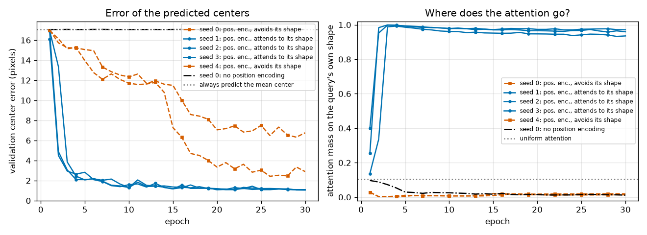
All five models with positional encoding do far better than the baseline (17.06 pixels). But in the right plot, the five seeds clearly split into two groups. This was not the expected result, but it is reported as is and examined below.
- The look-at-the-shape solution (seeds 1, 2, 3): attention on the assigned shape jumps close to 1 within two or three epochs and is 0.93–0.97 at epoch 30. The error also drops to 2–3 pixels within 5 epochs and ends at an average of 1.07 pixels.
- The look-at-everything-but-the-shape solution (seeds 0, 4): attention on the assigned shape is 0.014–0.019. That is far lower even than the 0.103 of uniform attention, so the query is deliberately avoiding that shape. Even so, the error decreases slowly, reaching 2.90 and 6.76 pixels at epoch 30 (and the curves are still going down).
- Figure: Figure 5-10 Attention maps of three models on two validation images (four panels on the left, four on the right). Each row is a different model: the first row is the look-at-the-shape solution (seed 1), the second row the look-at-everything-but-the-shape solution (seed 0), and the third row the model without positional encoding. A white + on the image is the ground-truth center, and a circle is the predicted center (outline color = assigned color). Each map shows the weight per patch on the 12×12 grid, brighter meaning larger (each map's color range runs from 0 to that map's maximum).
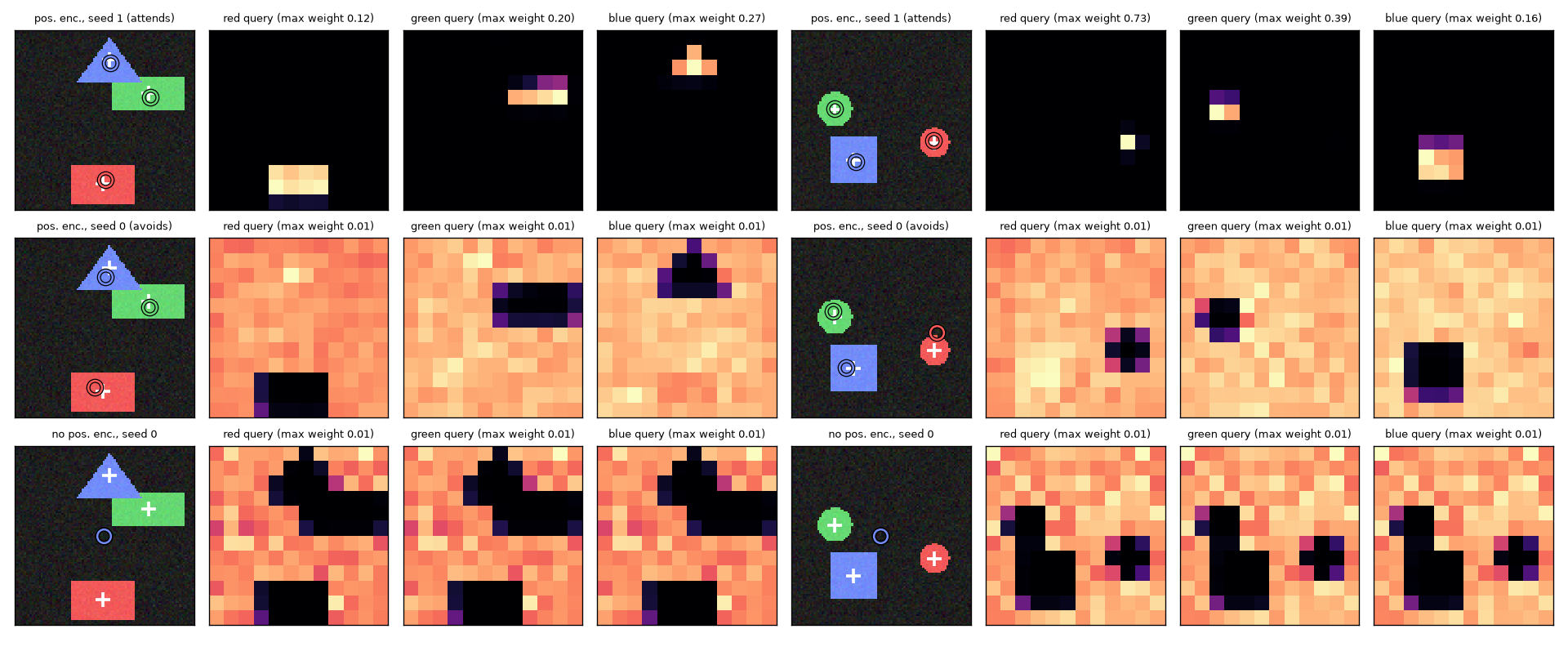
Let us read Figure 5-10 row by row.
- First row (looks at the shape): in the red query's map, only the patches with the red shape are bright and the rest are black. The green and blue queries likewise look only at their own shapes. The query searches for “something red”, and from the values of the tokens whose keys answered “I am red”, it fetches “I am here”. This is exactly the “find and fetch” described in this chapter, and the predicted circles sit on the + marks.
- Second row (looks at everything but the shape): the map is inverted. The whole image is evenly bright (the maximum weight is 0.01, close to the uniform value \(1/144 \approx 0.007\)), and only the assigned shape's area is blacked out.
How the second solution gets the position right can be explained by the fact that “the output is a weighted average of values”. Let \(T\) be the set of tokens covered by the assigned shape (\(n\) tokens). If the query looks evenly at the remaining \(N - n\) tokens, the output is
\(o = \frac{1}{N - n} \sum_{j \notin T} v_j = \frac{1}{N - n} \Big( \sum_{j=1}^{N} v_j - \sum_{j \in T} v_j \Big)\)
The positional information carried by the values, summed over all tokens, is the same for every image (the grid never changes). So what remains in the output is “what is missing from the whole”, that is, the position of the assigned shape. The model reads the position from the hole. However, the contents of the other two shapes are also mixed into the average, which blurs the signal; this is probably why this solution learned more slowly and had larger errors in this experiment.
Lessons from this experiment
- Attention can search by content (key: what color is it) and fetch different information (value: where is it). With three of the seeds, the queries put 93–97% of their weight on their own shapes.
- With the same architecture, the same data, and the same loss, entirely different attention maps can emerge depending on initialization. The loss only said “get the center right”; it never said “look at the shape”.
- So be careful when reading an attention map as “where the model thinks is important”. In the second solution's map only the assigned shape is black, yet that model is predicting exactly that shape's position.
This was observed in a toy model with one layer and one head. What about large detectors? The DETR paper visualizes the attention of its trained decoder (Figure 6 in the paper) and notes that queries mostly look at extremities of objects, such as heads and legs. That resembles the first solution.
Without positional encoding
The model without positional encoding (black dash-dot line, third row of Figure 5-10) learns nothing at all. Its validation error stays at 17.06–17.07 pixels for all 30 epochs, the same as the baseline of answering the average center without looking at the image (17.06). In the third row of Figure 5-10, the three queries' predicted circles overlap at a single point near the middle of the image.
The reason is exactly what the previous section derived. Without positional encoding, the tokens contain only the pixel content of their patches. A query may be able to find the red tokens, but nowhere in those tokens' values is there “I am here”. With no position information to fetch, the best answer is the average. The three queries' maps are nearly identical, and they avoid every place with a shape, whatever its color. This can be explained by the fact that, for answering the average, the shape tokens, which differ from image to image, only get in the way, so the queries end up looking only at the background.
This is also why the ViT in chapter 6 adds position embeddings to its patch tokens and why DETR in chapter 7 adds positional encodings in every attention layer.
Experiment: token count and time
Finally, let us confirm “the square of the token count” with a clock. We time one self-attention step with \(D = 256\) and 8 heads while varying the token count \(N\) from 144 to 4,096 (batch 1, a single CPU thread). Both the from-scratch MultiHeadAttention and the built-in nn.MultiheadAttention, set not to return weights, are timed.
def time_self_attention(token_counts, dim=256, heads=8, rounds=3, repeats=3, budget=1.0):
    """토큰 N 개의 자기 어텐션 한 번(배치 1)에 걸리는 시간(밀리초)을 잰다.

    - 계산량이 N 에 따라 어떻게 느는지만 깨끗이 보려고 CPU 의 스레드 하나로 잰다
      (GPU 나 여러 스레드로 재면 작은 N 에서는 일을 나눠 맡기는 고정 비용이 시간을 좌우한다).
    - 시계는 time.process_time: 이 프로그램이 CPU 를 실제로 쓴 시간만 센다(다른 프로그램에 CPU 를 내준 시간은 빠진다).
    - 모든 N 을 한 바퀴 재는 일을 rounds 번 되풀이하고, 설정마다 가장 빠른 값을 쓴다
      (다른 프로그램이 끼어들면 느려질 뿐 빨라지지는 않으므로, 최솟값이 방해를 가장 덜 받은 값이다).
    - 직접 구현(가중치 행렬 N × N 을 만들어 돌려준다)과 내장 모듈(need_weights=False → 가중치를 돌려주지 않아도 되므로
      내부에서 F.scaled_dot_product_attention 을 쓴다) 둘 다 잰다.
    """
    torch.manual_seed(0)
    mine = MultiHeadAttention(dim, heads).eval()
    builtin = copy_to_builtin(mine).eval()
    threads = torch.get_num_threads()
    torch.set_num_threads(1)

    def clock(fn):
        """적어도 repeats 번, 그리고 budget 초가 찰 때까지 되풀이해 가장 빠른 값(밀리초)."""
        times, t_end = [], time.perf_counter() + budget
        while len(times) < repeats + 1 or time.perf_counter() < t_end:
            t0 = time.process_time()
            fn()
            times.append((time.process_time() - t0) * 1000)
        return min(times[1:])  # 첫 번은 준비 운동이라 뺀다

    best = {n: [float("inf"), float("inf")] for n in token_counts}
    with torch.no_grad():
        for _ in range(rounds):
            for n in token_counts:
                x = torch.randn(1, n, dim)
                best[n][0] = min(best[n][0], clock(lambda: mine(x, x, x)))
                best[n][1] = min(best[n][1], clock(lambda: builtin(x, x, x, need_weights=False)))
    torch.set_num_threads(threads)  # 스레드 수를 되돌려 놓는다
    return [(n, best[n][0], best[n][1]) for n in token_counts]
[시간] N =   144 (쌍     20,736개): 직접 구현    0.906 ms, 내장(가중치 안 돌려줌)    0.903 ms
[시간] N =   576 (쌍    331,776개): 직접 구현    8.026 ms, 내장(가중치 안 돌려줌)    6.989 ms
[시간] N =  1024 (쌍  1,048,576개): 직접 구현   50.701 ms, 내장(가중치 안 돌려줌)   29.119 ms
[시간] N =  1600 (쌍  2,560,000개): 직접 구현  125.457 ms, 내장(가중치 안 돌려줌)   70.994 ms
[시간] N =  2304 (쌍  5,308,416개): 직접 구현  289.069 ms, 내장(가중치 안 돌려줌)  138.507 ms
[시간] N =  4096 (쌍 16,777,216개): 직접 구현  969.299 ms, 내장(가중치 안 돌려줌)  452.642 ms
[시간] N 이 144 → 4096 (28.4배, N² 은 809배)일 때 시간: 직접 구현 1069배, 내장 501배
[시간] 로그-로그 직선 맞춤의 기울기(시간 ∝ N^기울기): 직접 구현 2.14, 내장 1.88
- Figure: Figure 5-11 Time for one self-attention step versus token count \(N\) (both axes logarithmic). The solid blue line is the from-scratch implementation, the dashed orange line the built-in module, and the dashed gray line the slope (2) of something proportional to \(N^2\).
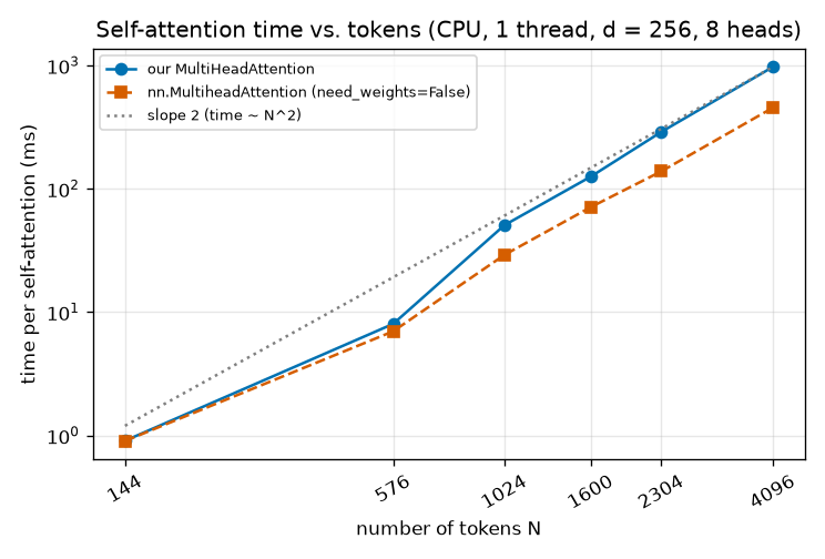
Here is what to read from the output and Figure 5-11.
- The overall trend is quadratic. When the tokens grow 28.4-fold from 144 to 4,096, the token pairs grow 809-fold, and the time grows 1,069-fold for the from-scratch implementation and 501-fold for the built-in module. On a log-log plot, the slope of a line is “the power of \(N\) at which time grows”, and the slopes fitted to the six points are 2.14 and 1.88, both near 2. Both curves run parallel to the dashed gray line (slope 2).
- The more tokens, the closer to quadratic. Quadrupling \(N\) from 1,024 to 4,096 (16 times the token pairs) makes the from-scratch implementation \(969.299 / 50.701 \approx 19.1\) times slower and the built-in module \(452.642 / 29.119 \approx 15.5\) times slower. In contrast, quadrupling from 144 to 576 gives only \(8.026 / 0.906 \approx 8.9\) times, short of 16. That is because an attention layer also does work that is simply proportional to \(N\). The four projections (\(W_Q, W_K, W_V, W_O\)) multiply each token by a \(D \times D\) matrix, about \(4 N D^2\) multiplications, while computing the scores takes about \(N^2 D\). The two are equal at \(N = 4D = 1{,}024\), so with fewer tokens than that the projections dominate the time, and with more the quadratic term does.
- The built-in module is faster. At \(N = 4{,}096\), the from-scratch implementation takes 969 ms and the built-in module 453 ms, about a factor of two. They compute the same formula, but since the built-in module does not have to return the weight matrix, it can choose an implementation that uses less memory. Still, the two curves are nearly parallel. Refining the implementation only reduces the constant factor; the quadratic growth stays.
A note on how the measurement was done: to see only the trend in computation, it measured the CPU time this program actually used, on a single CPU thread. The computer used to write this tutorial was running other work at the same time, so repeating the same measurement sometimes changed individual points by nearly a factor of two. So read the trend rather than the millisecond values themselves. On your computer the numbers will differ, but the slope should be near 2.
Going back to the earlier table, the backbones of RF-DETR N (576 tokens) and 2XL (1,936 tokens) pay this quadratic cost in every layer. If every token looked at every other token in every layer, the cost would jump steeply each time the resolution is raised. This is why the window attention of chapter 9 is needed.
F.scaled_dot_product_attention and Flash Attention
Since PyTorch 2.0, torch.nn.functional.scaled_dot_product_attention does the same job as the first function in this chapter. The last [check] line in the multi-head attention section confirmed that it gives the same result as our implementation. The built-in function computes the same formula but picks a faster implementation when one is available. A well-known one is Flash Attention (FlashAttention; Dao et al., 2022). Instead of materializing the whole \(N \times N\) weight matrix in memory, it computes in small blocks, reducing the amount of memory read and written while leaving the result unchanged. It is not an approximation; it produces the same values. In exchange, it does not return the weight matrix, so to draw attention maps you have to compute them yourself, as in this chapter.
The RF-DETR paper also mentions this optimization in Section 4 when comparing backbones. As the reason SAM2's Hiera backbone was not as fast as expected, it points out that Hiera did not account for “Flash Attention kernels that are highly optimized in compilers like TensorRT”. The point is that how fast attention runs depends not only on the formula but also on how well the deployment tooling has optimized that operation. Latency measurement is covered in chapter 12 and chapter 14.
Summary
- Attention lets every token see every token in a single layer. A token is one vector; in this tutorial it is an image patch or an object query.
- Scores come from dot products of queries and keys, softmax turns them into weights, and the values are averaged with those weights: \(\operatorname{Attention}(Q, K, V) = \operatorname{softmax}(QK^\top/\sqrt{d_k})\,V\). Shapes: \((N_q, d_k), (N_k, d_k), (N_k, d_v) \to (N_q, N_k) \to (N_q, d_v)\).
- If components are independent with variance 1, \(\operatorname{Var}(q \cdot k) = d_k\). Dividing by \(\sqrt{d_k}\) to bring the variance to 1 prevents the softmax from concentrating on one place from the start and killing the gradient \(\alpha(1 - \alpha)\).
- In self-attention, \(Q, K, V\) come from the same tokens; in cross-attention, \(Q\) and \(K, V\) come from different tokens. In the DETR decoder, object queries look at image tokens.
- The cost of self-attention is quadratic in the token count, \(O(N^2 D)\). Deformable attention in chapter 8 and window attention in chapter 9 reduce it.
- A mask adds \(-\infty\) to scores to make the weights exactly 0 (key padding mask, attention mask).
- Multi-head attention splits \(D\) into \(h\) heads (\(d_k = D/h\)), attends separately, and concatenates. It has \(4(D^2 + D)\) parameters regardless of the number of heads (263,168 for \(D = 256\)).
- Attention does not know order (\(f(PX) = Pf(X)\)). Adding sinusoidal positional encoding supplies position, and the dot product of two positional encodings depends only on the offset. Images use a 2D encoding with a \(y\) half and an \(x\) half.
- Transformer layer = attention + FFN, each with a residual connection and layer normalization. Post-norm is \(\operatorname{LN}(x + f(x))\); pre-norm is \(x + f(\operatorname{LN}(x))\). A decoder layer is self-attention → cross-attention → FFN.
- In this chapter's experiment, a single cross-attention layer found shapes by color and fetched their positions, and without positional encoding it got nothing right. Depending on the seed, a solution that “looks at everything but the shape” also appeared.
You now have attention and the Transformer layer as building blocks. In chapter 6, these blocks are used to build a backbone that reads images. Cut the image into patches, turn them into tokens, add learned position embeddings, and stack pre-norm encoder layers, and you have a Vision Transformer. The chapter also looks at why RF-DETR chose a ViT called DINOv2 as its backbone and what its pretraining is.
Review questions
- 1. (Attention by hand) The query is \(q = (2, 2)\), the keys are \(k_1 = (1, 0)\), \(k_2 = (0, 1)\), \(k_3 = (1, 1)\), and the values are single numbers \(v_1 = 10\), \(v_2 = 20\), \(v_3 = 30\) (\(d_k = 2\), \(d_v = 1\)). Find the scores, weights, and output. (\(e^{1.4142} = 4.113\), \(e^{2.8284} = 16.919\))
- The dot products are \((2, 2, 4)\), and dividing by \(\sqrt{2}\) gives scores \((1.4142, 1.4142, 2.8284)\). The exponentials are \((4.113, 4.113, 16.919)\), summing to \(25.145\). The weights are \((4.113/25.145,\; 4.113/25.145,\; 16.919/25.145) = (0.1636, 0.1636, 0.6728)\). The output is \(0.1636 \times 10 + 0.1636 \times 20 + 0.6728 \times 30 = 1.636 + 3.272 + 20.184 = 25.09\). It lies within the range of the three values 10, 20, 30 and leans toward the best-matching third one.
- 2. (Shape tracking) In cross-attention, 300 object queries look at 576 image tokens (\(D = 256\), 8 heads, batch 1). Give \(d_k\) for one head, the shape and number of entries of the weight tensor, and the shape of the output.
- \(d_k = 256/8 = 32\). The weights are
(1, 8, 300, 576), with \(8 \times 300 \times 576 = 1{,}382{,}400\) entries. The output follows the number of queries:(1, 300, 256). The 576 image tokens are unchanged. - 3. (When the variance is not 1) If all components of the query and key are independent with mean 0 and variance \(\sigma^2\), what is \(\operatorname{Var}(q \cdot k)\)? What should you divide by to make the score variance 1?
- In the derivation above, \(\mathbb{E}[a_m^2] = \mathbb{E}[c_m^2] = \sigma^2\) instead, so \(\operatorname{Var}(a_m c_m) = \sigma^2 \cdot \sigma^2 = \sigma^4\) and hence \(\operatorname{Var}(q \cdot k) = d_k\, \sigma^4\). Dividing by the standard deviation \(\sigma^2\sqrt{d_k}\) makes the variance 1. With \(\sigma = 1\) this is the same as the \(\sqrt{d_k}\) in the main text.
- 4. (Parameter count) Count the parameters of one Transformer encoder layer with \(D = 384\), 6 heads, and FFN expansion ratio \(r = 4\) (the size of ViT-S, which appears in chapter 6). Include biases and the two layer normalizations (one layer normalization has \(D\) scale and \(D\) shift parameters).
- Attention: \(4(D^2 + D) = 4 \times (147{,}456 + 384) = 591{,}360\). The head count 6 is not used. FFN: hidden size \(4 \times 384 = 1536\). \((384 \times 1536 + 1536) + (1536 \times 384 + 384) = 591{,}360 + 590{,}208 = 1{,}181{,}568\). Layer normalization: \(2 \times (384 + 384) = 1{,}536\). Total \(591{,}360 + 1{,}181{,}568 + 1{,}536 = 1{,}774{,}464\).
- 5. (Quadratic cost) A backbone with patch size 16 was fed images with side 384, then switched to 768. By what factor do the token count and the number of self-attention token pairs grow? What if the resolution stays at 384 and the patch size is reduced to 8?
- 384/16 = 24, so \(24^2 = 576\) tokens and 331,776 pairs. 768/16 = 48, so \(48^2 = 2{,}304\) tokens (4×) and 5,308,416 pairs (16×). At resolution 384 with patch 8, 384/8 = 48, giving the same grid. Since the token count is (side ÷ patch size)², doubling the resolution and halving the patch increase the cost by exactly the same amount.
- 6. (Masks) A query's weights were \((0.5, 0.3, 0.2)\). What are the weights if the second key is masked? Explain why this can be computed without knowing the scores.
- \((0.5/0.7,\; 0,\; 0.2/0.7) = (0.714,\; 0,\; 0.286)\). The weights have the form \(\alpha_j = e^{s_j}/C\) (\(C\) is the sum of the exponentials), so the ratio of \(e^{s_j}\) among unmasked keys equals the ratio of their weights, \(0.5 : 0.2\). The mask removes only the second term from the denominator, which is the same as renormalizing the remaining weights by their sum \(0.5 + 0.2 = 0.7\).
- 7. (Positional encoding) For the 1D sinusoidal positional encoding with \(D = 4\), compute \(PE(0) \cdot PE(2)\) in two ways: (a) by directly taking the dot product of the vectors in the table above, and (b) with the formula \(\sum_i \cos(\omega_i \Delta)\). (\(\cos 2 = -0.4161\), \(\cos 0.02 = 0.9998\))
- (a) \(PE(0) = (0, 1, 0, 1)\) and \(PE(2) = (0.9093, -0.4161, 0.0200, 0.9998)\), so the dot product is \(0 - 0.4161 + 0 + 0.9998 = 0.5837\). (b) With offset \(\Delta = 2\), \(\omega_0 = 1\), \(\omega_1 = 0.01\): \(\cos(2) + \cos(0.02) = -0.4161 + 0.9998 = 0.5837\). They agree, and the value is smaller than the dot product with itself, \(D/2 = 2\).
- 8. (Order and position) After several self-attention layers without positional encoding, the outputs of all tokens are averaged into a single vector for the whole image. What happens to this vector if the image's patches are fed in shuffled at random? Which can this model predict: “is there a red shape in the image?” or “is the red shape on the left?”
- Self-attention layers are permutation equivariant, so shuffling the input only shuffles the per-token outputs in the same order, and the average does not depend on order, so the vector does not change at all (permutation invariance). The model can therefore predict things determined by patch content alone, like “is there a red shape?”, but not “is it on the left?”, because it must give the same answer for the image before and after shuffling. This is the same reason the model without positional encoding in the experiment never moved a step beyond the baseline.
See also
Favorite site
- 05. Attention and Transformer
- ch05_attention.py - practice code for this chapter
- World Model tutorial, chapter 2: Probability - proofs of the expectation and variance properties
- Attention Is All You Need (Vaswani et al., 2017)
- End-to-End Object Detection with Transformers (DETR)
- An Image is Worth 16x16 Words (ViT)
- FlashAttention (Dao et al., 2022)
- RF-DETR paper