RF-DETR:Tutorial:04-DeepLearningBasics
lastmod 2026-11-18created 2026-11-1818 edits
Deep learning basics and classification loss is chapter 4 of the RF-DETR tutorial. Chapters 2 and 3 covered how to measure boxes and how to score detectors, so before building a detector, this chapter reviews the deep learning components that later chapters use without explanation. It skims linear layers and activation functions (ReLU, GELU, SiLU), backpropagation by hand and autograd, SGD → Adam → AdamW, normalization layers (batch and layer normalization), residual connections, and convolution. It then follows classification loss (sigmoid and logits, BCE derived from Bernoulli maximum likelihood and its gradient \(p - y\), the numerically stable form, soft targets, softmax + background class versus per-class sigmoid, focal loss, and prior-probability bias initialization) without skipping a single line of the derivations, because the detector losses in chapters 7, 9, and 11 are all small variations of the formulas in this chapter. The chapter ends by training a classification problem in the shapes world, where only 0.6% of the samples are positive, under three settings and comparing the results.
- Original: 04. Deep Learning Basics and Classification Loss
- Practice code: a single file,
code/ch04_basics.py. Running it once prints results [1] through [10] in order. The full run takes 5 min 40 s on an 8 GB laptop GPU (mostly the [9] experiment at the end of the chapter); the reduced version with--quicktakes about 20 seconds. Reading time about 90 minutes, difficulty ★★☆☆☆. - Previous: 03. Scoring Detectors: AP and mAP / Next: 05. Attention and Transformer
How to read this chapter
A longer, from-scratch explanation of neural networks, differentiation, backpropagation, and convolution is in chapter 4, “Deep Learning and PyTorch Basics” of the World Model tutorial. This chapter re-explains just enough that you can follow along without reading it, but keeps the overlapping material short and spends its length on the classification loss that detectors need. If you are already comfortable with deep learning, you can start from “Classification ①: sigmoid and logits”.
A neural network is a function with parameters
A neural network is a function \(f_\theta(x)\) that takes an input \(x\) and produces an output. The subscript \(\theta\) (theta) is a collective name for the adjustable numbers inside the function, i.e., the parameters. For a detector, \(x\) is an image and the output is “boxes and class scores”. The \(\theta\) of RF-DETR (nano) consists of about 30.5 million numbers (Table 2 of the paper). Training means adjusting \(\theta\) little by little so that the output gets closer to the ground truth, and the first half of this chapter is about how that adjustment is done.
Linear layers and shape arithmetic
The smallest building block of a neural network is the linear layer (fully connected layer). It takes a vector \(x\) of \(n\) numbers and outputs a vector \(h\) of \(m\) numbers.
\(h = Wx + b, \qquad x \in \mathbb{R}^{n},\quad W \in \mathbb{R}^{m \times n},\quad b \in \mathbb{R}^{m},\quad h \in \mathbb{R}^{m}\)
\(W\) is the weight matrix (\(m\) rows, \(n\) columns) and \(b\) is the bias vector. The \(i\)-th number of \(h\) is “the sum of the elementwise products of the \(i\)-th row of \(W\) and \(x\), plus \(b_i\)”. The parameters are the \(m \times n\) entries of \(W\) and the \(m\) entries of \(b\), \(mn + m\) in total.
- Worked example — a linear layer that takes 3 numbers and outputs 2
- \(W = \begin{pmatrix} 1 & 0 & -1 \\ 2 & 1 & 0 \end{pmatrix},\quad x = \begin{pmatrix} 1 \\ 2 \\ 3 \end{pmatrix},\quad b = \begin{pmatrix} 0.5 \\ -1 \end{pmatrix}\)
- Since \(n = 3\) and \(m = 2\), \(W\) has 2 rows and 3 columns. That makes \(2 \times 3 + 2 = 8\) parameters.
- Multiply the first row of \(W\), \((1, 0, -1)\), elementwise by \(x\), sum, and add \(b_1 = 0.5\).
- Multiply the second row \((2, 1, 0)\) elementwise by \(x\), sum, and add \(b_2 = -1\).
- In terms of shapes, this is \((3,) \to (2,)\).
In PyTorch, nn.Linear(n, m) applies this computation only to the last axis of the input and leaves the leading axes as they are. So if the input is (B, n) the output is (B, m), and if the input is (B, N, n) the output is (B, N, m). For example, RF-DETR's classification head is a single nn.Linear(256, 클래스 수) (chapter 10). Each of the B images has 300 prediction slots, each holding a 256-dimensional vector, so with 80 classes the shape goes (B, 300, 256) → (B, 300, 80) and there are \(256 \times 80 + 80 = 20{,}560\) parameters. Each individual cell of this (B, 300, 80) output is the protagonist of the second half of this chapter.
Activation functions: ReLU · GELU · SiLU
Stacking only linear layers, however many, is equivalent to a single linear layer, because \(W_2(W_1 x + b_1) + b_2 = (W_2 W_1)x + (W_2 b_1 + b_2)\). So between layers we insert a nonlinear function, the activation function, applied to each number independently. This tutorial uses three activation functions.
| Name | Formula | At \(x = -1\) | At \(x = 1\) | Where RF-DETR uses it |
| ReLU(rectified linear unit) | \(\max(0, x)\) | \(0\) | \(1\) | FFN in the decoder (chapter 5, chapter 10) |
| GELU(Gaussian error linear unit) | \(x \cdot \Phi(x)\) | \(-0.1587\) | \(0.8413\) | FFN in the ViT (DINOv2) backbone (chapter 6) |
| SiLU(sigmoid linear unit, Swish) | \(x \cdot \sigma(x)\) | \(-0.2689\) | \(0.7311\) | C2f blocks in the projector (chapter 9) |
\(\Phi(x)\) (Phi) is the cumulative distribution function of the standard normal distribution, i.e., “the probability that a number drawn from a bell-shaped distribution with mean 0 and standard deviation 1 is at most \(x\)” (\(\Phi(0) = 0.5\), \(\Phi(1) = 0.8413\)). \(\sigma(x) = 1/(1 + e^{-x})\) is the sigmoid, covered in detail later (\(\sigma(1) = 0.7311\)). Both are curves that rise smoothly from 0 to 1, so GELU and SiLU can be viewed as smooth ReLUs in which “\(x\) itself decides how much of \(x\) to let through”.
def relu(x: torch.Tensor) -> torch.Tensor:
    """ReLU(x) = max(0, x). 음수는 0 으로, 양수는 그대로."""
    return torch.clamp(x, min=0.0)

def gelu(x: torch.Tensor) -> torch.Tensor:
    """GELU(x) = x · Φ(x). Φ 는 표준 정규 분포의 누적 분포 함수: Φ(x) = (1 + erf(x / √2)) / 2."""
    return x * 0.5 * (1.0 + torch.erf(x / math.sqrt(2.0)))

def silu(x: torch.Tensor) -> torch.Tensor:
    """SiLU(x) = x · σ(x). σ 는 시그모이드. Swish 라고도 부른다."""
    return x * torch.sigmoid(x)
- Figure: Figure 4-1 The three activation functions (left) and their derivatives (right). Solid line: ReLU; dashed line: GELU; dash-dotted line: SiLU.
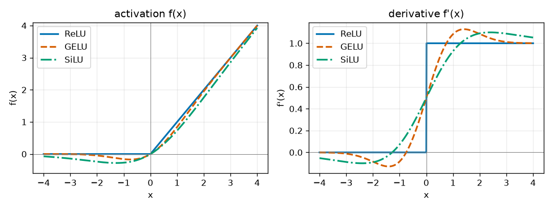
There are three things to take from Figure 4-1.
- For large positive inputs, the three are nearly identical. At \(x = 3\), ReLU gives 3, GELU 2.9960, and SiLU 2.8577.
- They differ near 0. ReLU has a kink at 0, and its derivative on the negative side is exactly 0. As long as the input is negative, no gradient at all flows through that position. GELU and SiLU continue smoothly without a kink, dip slightly below zero on the negative side (the minimum is \(-0.1700\) at \(x = -0.7518\) for GELU and \(-0.2785\) at \(x = -1.2785\) for SiLU), and then return to 0.
- There is a range where the derivative slightly exceeds 1 (right panel). This comes from GELU and SiLU dipping and coming back up on the negative side, and it causes no problems.
Which one is better depends on the architecture and the data, so this tutorial follows the policy of “use whatever the original model uses”.
The code for this chapter is a single file (code/ch04_basics.py), and running it once prints results [1] through [10] in order. From here on, that output is shown piece by piece in the relevant sections. The full run took 5 min 40 s on an 8 GB laptop GPU that was also being used for other work (mostly the [9] experiment at the end of the chapter); the reduced version with --quick takes about 20 seconds.
[1] 활성 함수: ReLU · GELU · SiLU
  x        -3.0000   -1.0000    0.0000    1.0000    3.0000
  ReLU      0.0000    0.0000    0.0000    1.0000    3.0000   | check: 내장과의 최대 차이 0.0e+00
  GELU     -0.0040   -0.1587    0.0000    0.8413    2.9960   | check: 내장과의 최대 차이 1.8e-07
  SiLU     -0.1423   -0.2689    0.0000    0.7311    2.8577   | check: 내장과의 최대 차이 2.4e-07
  GELU 의 최솟값 -0.1700 (x = -0.7518)
  SiLU 의 최솟값 -0.2785 (x = -1.2785)
The three hand-written functions match the PyTorch built-ins (F.relu, F.gelu, F.silu) within rounding error (\(10^{-7}\), float32), and the values in the table and the minima mentioned above come out exactly.
MLP: stacked layers
A neural network built as “linear layer → activation function → linear layer → …” is called an MLP (multi-layer perceptron). Writing the activation function as \(\phi\) (phi), a 2-layer MLP is:
\(f_\theta(x) = W_2\,\phi(W_1 x + b_1) + b_2, \qquad \theta = \{W_1, b_1, W_2, b_2\}\)
The middle part \(\phi(W_1 x + b_1)\) is an intermediate value that is not visible from the outside, so it is called the hidden vector. In later chapters, MLPs appear under two names: the FFN inside a Transformer block (chapter 5: one activation function between two linear layers), and the box head that produces 4 box coordinates from a 256-dimensional vector (chapter 7: a 3-layer MLP).
Loss and gradient descent
Loss functions and gradients
A loss function \(L\) measures, as a single number, how far the network's output is from the ground truth. Smaller is better. With the data fixed, the loss becomes a function \(L(\theta)\) of the parameters \(\theta\) alone, and training becomes “finding the \(\theta\) that makes \(L(\theta)\) small”.
The method is simple. For each parameter, compute “how much the loss changes if this number is increased very slightly”. That is the partial derivative \(\frac{\partial L}{\partial \theta_i}\), and the vector of the partial derivatives for all parameters is called the gradient \(\nabla_\theta L\) (nabla). The gradient points in the direction in which the loss increases fastest, so moving a little in the opposite direction reduces the loss.
\(\theta \leftarrow \theta - \eta\, \nabla_\theta L(\theta)\)
This is gradient descent. \(\eta\) (eta) is the learning rate, which sets how far to move in one step. If it is too large, the step overshoots the valley and the loss actually grows; if it is too small, training never finishes. RF-DETR's default learning rate is \(10^{-4}\), deliberately set small to avoid wrecking the pretrained backbone (chapter 11). The derivation of why the direction opposite the gradient reduces the loss, and of the learning rate above which training diverges, is in the “Gradient descent” section of chapter 4 of the World Model tutorial.
The chain rule and backpropagation by hand
How do we get the gradient of a network with tens of millions of parameters? The only tool needed is the rule for differentiating composite functions from high school, i.e., the chain rule. If \(L\) is a function of \(q\) and \(q\) is a function of \(r\), then
\(\frac{\partial L}{\partial r} = \frac{\partial L}{\partial q} \cdot \frac{\partial q}{\partial r}\)
In words: “the effect of \(r\) on \(L\) = (the effect of \(q\) on \(L\)) × (the effect of \(r\) on \(q\))”. A neural network is a chain of computations, so starting from the loss and going backward one step at a time, passing along (incoming gradient) × (local derivative of this step), yields the gradients of all parameters. Computing values from the input to the loss is the forward pass; computing gradients backward from the loss is backpropagation.
Let's work through a 2-layer network in which only a single number flows at each point.
| Part | Formula | Values |
| Input and target | \(x\), \(y\) | \(x = 2\), \(y = 1\) |
| Layer 1 | \(u = w_1 x + b_1\), \(h = \max(0, u)\) | \(w_1 = 0.5\), \(b_1 = 0.1\) |
| Layer 2 | \(\hat{y} = w_2 h + b_2\) | \(w_2 = -1.5\), \(b_2 = 0.2\) |
| Loss | \(L = (\hat{y} - y)^2\) |
\(\hat{y}\) (y-hat) is the network's prediction, \(u\) is the value before the activation function, and \(h\) is the hidden value.
Figure 4-2 in the original is the computation graph of this network. The five values \(x \to u \to h \to \hat{y} \to L\) are connected from left to right, and each arrow is labeled with its computation: \(\times w_1 + b_1\), ReLU, \(\times w_2 + b_2\), and \((\hat{y} - y)^2\). Above are the values from the forward pass (\(x = 2\), \(u = 1.1\), \(h = 1.1\), \(\hat{y} = -1.45\), \(L = 6.0025\)), and below are the gradients from backpropagation (\(\partial L/\partial L = 1\), \(\partial L/\partial \hat{y} = -4.9\), \(\partial L/\partial h = 7.35\), \(\partial L/\partial u = 7.35\)). Under each arrow are the gradients of the parameters that arrow contains (\(\partial L/\partial w_1 = 14.7\), \(\partial L/\partial b_1 = 7.35\), \(\partial L/\partial w_2 = -5.39\), \(\partial L/\partial b_2 = -4.9\)). Forward values flow from left to right, and backpropagated gradients flow from right to left.
- Forward pass — from the input to the loss
- \(u = w_1 x + b_1 = 0.5 \cdot 2 + 0.1 = 1.1\)
- The linear computation of layer 1.
- ReLU. \(u\) is positive, so it passes through unchanged.
- The linear computation of layer 2.
- The prediction is a full 2.45 away from the target of 1.
- Backpropagation — backward from the loss, (incoming gradient) × (local derivative)
- \(\frac{\partial L}{\partial \hat{y}} = 2(\hat{y} - y) = 2 \cdot (-2.45) = -4.9\)
- The derivative of \(L = (\hat{y} - y)^2\) with respect to \(\hat{y}\). It is negative, meaning “increasing \(\hat{y}\) decreases the loss”.
- From \(\hat{y} = w_2 h + b_2\), \(\frac{\partial \hat{y}}{\partial w_2} = h\) and \(\frac{\partial \hat{y}}{\partial b_2} = 1\). This gives the parameter gradients of layer 2.
- From the same formula, \(\frac{\partial \hat{y}}{\partial h} = w_2\). This value is passed back to layer 1.
- The derivative of ReLU is 1 if \(u \gt 0\) and 0 if \(u \lt 0\). Here \(u = 1.1 \gt 0\), so it is 1. Had \(u\) been negative, the gradient would become 0 at this point and layer 1 would learn nothing.
- From \(u = w_1 x + b_1\), \(\frac{\partial u}{\partial w_1} = x\) and \(\frac{\partial u}{\partial b_1} = 1\). The gradients of all four parameters are now known.
Applying one step of gradient descent with learning rate \(\eta = 0.01\) gives \(w_1 = 0.5 - 0.01 \cdot 14.7 = 0.353\), \(b_1 = 0.1 - 0.0735 = 0.0265\), \(w_2 = -1.5 + 0.0539 = -1.4461\), and \(b_2 = 0.2 + 0.049 = 0.249\), and redoing the forward pass with the new parameters reduces the loss from \(6.0025 \to 3.2771\).
Checking against autograd
PyTorch records which computations were performed during the forward pass, and a single .backward() call then performs the backpropagation above for you (autograd). So we only need to write the forward pass. Below, the hand computation above translated into code is placed side by side with autograd.
x, y = 2.0, 1.0  # 입력과 정답
w1, b1, w2, b2 = 0.5, 0.1, -1.5, 0.2  # 매개변수 네 개

# 순전파: 값을 왼쪽에서 오른쪽으로
u = w1 * x + b1  # 1층의 선형 계산
h = max(u, 0.0)  # ReLU
y_hat = w2 * h + b2  # 2층
loss = (y_hat - y) ** 2

# 역전파: 손실에서 거꾸로, (받은 기울기) × (국소 미분)
d_yhat = 2 * (y_hat - y)  # ∂L/∂ŷ
d_w2 = d_yhat * h  # ŷ = w2·h + b2 → ∂ŷ/∂w2 = h
d_b2 = d_yhat * 1.0  # ∂ŷ/∂b2 = 1
d_h = d_yhat * w2  # ∂ŷ/∂h = w2
d_u = d_h * (1.0 if u > 0 else 0.0)  # ReLU 의 미분: u > 0 이면 1, 아니면 0
d_w1 = d_u * x  # u = w1·x + b1 → ∂u/∂w1 = x
d_b1 = d_u * 1.0
params = torch.tensor([w1, b1, w2, b2], dtype=torch.float64, requires_grad=True)
tw1, tb1, tw2, tb2 = params.unbind()
t_loss = (tw2 * torch.relu(tw1 * x + tb1) + tb2 - y) ** 2  # 순전파만 적는다
t_loss.backward()  # 역전파는 autograd 가 한다
[2] 역전파 손계산 ↔ autograd (2층, 스칼라)
  순전파: u=1.1000 h=1.1000 ŷ=-1.4500 L=6.0025
  손계산: dL/dw1=14.7000 dL/db1=7.3500 dL/dw2=-5.3900 dL/db2=-4.9000
  autograd: dL/dw1=14.7000 dL/db1=7.3500 dL/dw2=-5.3900 dL/db2=-4.9000
  check: 손계산과 autograd 의 최대 차이 0.0e+00
  경사 하강 한 스텝(η=0.01): w1=0.3530 b1=0.0265 w2=-1.4461 b2=0.2490 → L=3.2771 (전 6.0025)
The hand computation and autograd agree to the last decimal place. Backpropagation is not new mathematics; it is simply the chain rule applied in order from the back. A hand computation for a 2-layer network whose hidden value is a vector is in “Backpropagation: computing a 2-layer network by hand” in chapter 4 of the World Model tutorial.
Mini-batches and optimizers
Mini-batches, steps, and epochs
The loss is usually an average over the whole dataset. But looking at all of tens of thousands of images for every single parameter update is wasteful. So we randomly draw \(B\) images from the data (a mini-batch) and perform one update using the gradient of their average loss. Three terms to pin down:
- Batch size \(B\): the number of images fed in at once.
- Step: one update of the parameters.
- Epoch: one full pass over the training data.
The experiment at the end of this chapter groups 2,000 images into batches of 32, so one epoch is \(\lfloor 2000 / 32 \rfloor = 62\) steps (\(\lfloor\cdot\rfloor\) means discarding the fractional part; the 16 leftover images are not used in that epoch). The mini-batch gradient is a “noisy estimate” of the full-data gradient, and the smaller the batch, the larger the noise. Gradient descent with mini-batch gradients is called SGD (stochastic gradient descent).
From SGD to Adam
SGD uses the same learning rate for every parameter. In a neural network, however, gradient magnitudes differ across parameters by factors of thousands. Adam (adaptive moment estimation; Kingma & Ba, 2015) keeps a separate record, for each parameter, of “which direction the gradient has pointed on average lately” and “how large the gradient has been lately”, and moves by scaling large gradients down and small gradients up. Writing the gradient at step \(n\) as \(g_n\),
\(\begin{aligned} m_n &= \beta_1 m_{n-1} + (1 - \beta_1)\, g_n && \text{(기울기의 지수 이동 평균: 방향)} \\ v_n &= \beta_2 v_{n-1} + (1 - \beta_2)\, g_n^2 && \text{(기울기 제곱의 지수 이동 평균: 크기)} \\ \hat{m}_n &= \frac{m_n}{1 - \beta_1^{\,n}}, \quad \hat{v}_n = \frac{v_n}{1 - \beta_2^{\,n}} && \text{(0 에서 시작한 탓에 작게 나온 것을 보정)} \\ \theta_n &= \theta_{n-1} - \eta\, \frac{\hat{m}_n}{\sqrt{\hat{v}_n} + \epsilon} && \text{(갱신)} \end{aligned}\)
The lines are, in order: the exponential moving average of the gradient (direction), the exponential moving average of the squared gradient (magnitude), the correction for values that come out too small because they start at 0, and the update. They start from \(m_0 = v_0 = 0\), and the defaults are \(\beta_1 = 0.9\), \(\beta_2 = 0.999\) (beta), and \(\epsilon = 10^{-8}\) (epsilon: a small number that prevents division by zero). Every computation is done separately for each parameter. The key is the division in the last line. Working out the first step (\(n = 1\)) by hand shows what happens.
- Adam's first step does not depend on the size of the gradient
- \(m_1 = (1 - \beta_1)\, g_1, \qquad v_1 = (1 - \beta_2)\, g_1^2\)
- Since \(m_0 = v_0 = 0\), the first terms vanish.
- The correction term exactly cancels \((1 - \beta)\).
- \(\sqrt{g_1^2} = |g_1|\), and \(\epsilon\) is tiny, so it is ignored. Whether the gradient is 10 or 0.001, the parameter decreases by exactly \(\eta\) if the gradient is positive and increases by \(\eta\) if it is negative.
Adam erases the magnitude of the gradient and keeps only its direction (and how consistent that direction is). As a result, multiplying the loss by a constant barely changes the update, and Transformers, whose gradient magnitudes vary widely from layer to layer, become easier to train. Momentum and bias correction are explained in detail in “Mini-batches, SGD, and Adam” in chapter 4 of the World Model tutorial.
AdamW: decoupling weight decay from the gradient
Weight decay pulls the weights slightly toward 0 at every step so that they do not grow needlessly large. Its strength is set by \(\lambda\) (lambda). There are two ways to add it; for SGD they are the same, but for Adam they differ.
| Method | What it does | Formula |
| L2 penalty (Adam + L2) | Adds \(\frac{\lambda}{2}\theta^2\) to the loss → \(\lambda\theta\) is added to the gradient | Replace \(g_n \leftarrow g_n + \lambda\,\theta_{n-1}\), then run the Adam above unchanged |
| Decoupled decay (AdamW: Adam with decoupled weight decay) | Leaves the gradient untouched and shrinks the weights separately | \(\theta_n = \theta_{n-1} - \eta\lambda\,\theta_{n-1} - \eta\, \dfrac{\hat{m}_n}{\sqrt{\hat{v}_n} + \epsilon}\) |
In the first method, the decay term \(\lambda\theta\) is mixed into the gradient, passes through \(m\) and \(v\), and is divided by \(\sqrt{\hat{v}}\). Since Adam is designed to erase the magnitude of the gradient, the magnitude of the decay is erased along with it. The second method (Loshchilov & Hutter, 2019) puts the decay outside that division. This is what “decoupled from the gradient” refers to. Let's compute the first step with a weight \(\theta = 1\), \(\eta = 0.01\), and \(\lambda = 0.1\).
- Worked example — the first step for a weight with gradient 10 and a weight with gradient 0.001
- \(\text{감쇠 없음:}\quad \theta_1 = 1 - \eta \cdot \frac{g_1}{|g_1|} = 1 - 0.01 = 0.99\)
- No decay. As shown above, the first step keeps only the sign of the gradient. Both weights become 0.99.
- \(\lambda\theta = 0.1\) was added to the gradient, but the sign is still positive and the magnitude is erased by the division. Even with decay added, the result is the same as without it.
- The second term is the Adam update. Both weights shrink by \(\eta\lambda = 0.1\%\) regardless of the size of their gradients. The decay works as intended, “in proportion to the size of the weight”.
The situation is the same after the first step. In Adam + L2, the decay is mixed with the loss gradient and divided by \(\sqrt{\hat{v}}\), so the larger a weight's loss gradient, the weaker its decay becomes in relative terms. AdamW shrinks every weight by the same factor \((1 - \eta\lambda)\) at every step. Nearly all Transformer-family models are trained with AdamW, and RF-DETR also uses AdamW (weight decay \(10^{-4}\)).
def adam_step(theta, grad, state, lr=0.01, beta1=0.9, beta2=0.999, eps=1e-8, weight_decay=0.0, decoupled=True):
    """Adam 한 스텝. theta · grad 는 모양이 같은 텐서, state 는 {"m", "v", "n"} 사전.

    weight_decay = λ 를 넣는 방법이 둘이다.
      decoupled=False (Adam + L2): 기울기에 λ·θ 를 더한다 → 감쇠 항도 √v̂ 로 나뉜다.
      decoupled=True  (AdamW)    : 기울기는 그대로 두고, θ 를 따로 (1 − η·λ) 배로 줄인다.
    """
    if weight_decay and not decoupled:
        grad = grad + weight_decay * theta  # L2 벌점 (λ/2)·θ² 의 기울기 λ·θ 를 손실 기울기에 섞는다
    if weight_decay and decoupled:
        theta = theta - lr * weight_decay * theta  # 기울기와 분리된 감쇠: θ ← (1 − η·λ)·θ
    state["n"] += 1
    state["m"] = beta1 * state["m"] + (1 - beta1) * grad  # 1차 모멘트: 기울기의 지수 이동 평균
    state["v"] = beta2 * state["v"] + (1 - beta2) * grad**2  # 2차 모멘트: 기울기 제곱의 지수 이동 평균
    m_hat = state["m"] / (1 - beta1 ** state["n"])  # 0 에서 시작한 탓에 작게 나온 것을 보정
    v_hat = state["v"] / (1 - beta2 ** state["n"])
    return theta - lr * m_hat / (v_hat.sqrt() + eps)
[3] Adam · Adam+L2 · AdamW 한 스텝 (θ=1, η=0.01, λ=0.1)
  Adam (감쇠 없음): 기울기 10 인 가중치 → 0.990000, 기울기 0.001 인 가중치 → 0.990000
  Adam + L2      : 기울기 10 인 가중치 → 0.990000, 기울기 0.001 인 가중치 → 0.990000
  AdamW          : 기울기 10 인 가중치 → 0.989000, 기울기 0.001 인 가중치 → 0.989000
  check: 직접 구현한 Adam+L2 20 스텝 vs torch.optim 최대 차이 1.1e-16
  check: 직접 구현한 AdamW 20 스텝 vs torch.optim 최대 차이 1.1e-16
The numbers match the hand computation, and applying the hand-written step 20 times in a row agrees with torch.optim.Adam(weight_decay=…) and torch.optim.AdamW to within \(10^{-16}\).
Classification ①: sigmoid and logits
At each prediction slot, a detector has to answer yes/no questions such as “Is there a cat here?” and “Is there a car here?”. The value that comes out of the network's last linear layer can be any real number from \(-\infty\) to \(+\infty\), so we need a function that converts it into a probability between 0 and 1.
Definition of the sigmoid and two properties
That function is the sigmoid (logistic function) \(\sigma\) (sigma). The real number \(z\) before it is converted into a probability is called the logit.
\(p = \sigma(z) = \frac{1}{1 + e^{-z}}\)
If \(z\) is very large, \(e^{-z} \to 0\) and so \(p \to 1\); if \(z\) is very small (a large negative number), \(e^{-z} \to \infty\) and so \(p \to 0\); and if \(z = 0\), \(p = \frac{1}{1 + 1} = 0.5\). A few values computed now will come in handy later: \(\sigma(2) = \frac{1}{1 + e^{-2}} = \frac{1}{1 + 0.1353} = 0.8808\), \(\sigma(-2) = \frac{1}{1 + e^{2}} = \frac{1}{1 + 7.3891} = 0.1192\). The graph is on the left of Figure 4-4 further below.
- Property 1 — \(\sigma(-z) = 1 - \sigma(z)\)
- \(\sigma(-z) = \frac{1}{1 + e^{z}}\)
- Substitute \(-z\) for \(z\) in the definition.
- Multiply the numerator and denominator by \(e^{-z}\). \(e^{-z} \cdot e^{z} = 1\).
- Write the numerator \(e^{-z}\) as \((1 + e^{-z}) - 1\) and split the fraction in two.
- If the probability of “yes” is \(\sigma(z)\), the probability of “no” is \(\sigma(-z)\). In numbers: \(\sigma(2) + \sigma(-2) = 0.8808 + 0.1192 = 1\).
- Property 2 — \(\sigma'(z) = \sigma(z)\,(1 - \sigma(z))\)
- \(\sigma(z) = (1 + e^{-z})^{-1}\)
- Write the fraction as a power.
- Chain rule. The derivative of the outer \(q^{-1}\) is \(-q^{-2}\), and the derivative of the inner \(1 + e^{-z}\) is \(-e^{-z}\).
- The two negatives cancel, and the fraction is split in two.
- The first factor is \(\sigma(z)\), and the second is \(\frac{e^{-z}}{1 + e^{-z}} = 1 - \sigma(z)\), seen in the derivation of Property 1. In numbers: \(\sigma'(2) = 0.8808 \times 0.1192 = 0.1050\), \(\sigma'(0) = 0.5 \times 0.5 = 0.25\) (the maximum).
Property 2 is easiest to remember as “the derivative of \(p\) with respect to \(z\) is \(p(1 - p)\)”. When \(p\) is close to 0 or 1, this value approaches 0: when the sigmoid is confident in one direction, moving the logit barely changes the probability.
The logit is the log-odds
Conversely, given a probability \(p\), what is the logit \(z\)? Solve the sigmoid for \(z\).
- The inverse of the sigmoid
- \(p = \frac{1}{1 + e^{-z}} \;\Longrightarrow\; 1 + e^{-z} = \frac{1}{p}\)
- Take the reciprocal of both sides.
- Move the 1 to the other side and put everything over a common denominator.
- Take the (natural) logarithm of both sides and move the sign. \(-\log\frac{a}{b} = \log\frac{b}{a}\).
\(\frac{p}{1 - p}\) is “the probability that it happens ÷ the probability that it does not”, called the odds. A probability of 0.8 gives odds of \(0.8 / 0.2 = 4\) (“4 to 1”). The logit is the logarithm of the odds, the log-odds. A table gives a feel for it.
| Probability \(p\) | 0.01 | 0.1192 | 0.5 | 0.8808 | 0.99 |
| Odds \(p/(1-p)\) | \(1/99\) | \(0.1353\) | \(1\) | \(7.389\) | \(99\) |
| Logit \(z\) | \(-4.5951\) | \(-2\) | \(0\) | \(2\) | \(4.5951\) |
The number \(z = \log\frac{0.01}{0.99} = -\log 99 = -4.5951\) for \(p = 0.01\) comes up again in “Prior-probability bias initialization”. This inverse function is also used again in chapter 8 under the name “inverse sigmoid” when handling box coordinates.
Classification ②: binary cross-entropy
We need a loss that measures how well the network's probability \(p\) agrees with the ground truth \(y\) (\(y = 1\) for “yes”, \(y = 0\) for “no”). In detection, a cell with \(y = 1\) is called a positive and a cell with \(y = 0\) a negative. This loss is not chosen arbitrarily; it follows from a probabilistic model.
From Bernoulli maximum likelihood to BCE
A distribution that gives “yes” with probability \(p\) and “no” with probability \(1 - p\) is called a Bernoulli distribution (tossing a bent coin). When the network outputs \(p\), the probability of getting the actual ground truth \(y\) is called the likelihood, and choosing the parameters that make the likelihood as large as possible is maximum likelihood estimation (MLE). It means “a model that assigns high probability to the ground truth is a good model”.
- Negative log of the Bernoulli likelihood = binary cross-entropy
- \(P(y \mid p) = \begin{cases} p & (y = 1) \\ 1 - p & (y = 0) \end{cases}\)
- The definition of the Bernoulli distribution: the probability of the ground truth \(y\) when the network outputs \(p\).
- A trick for writing both cases in one line. If \(y = 1\), \(p^1 (1-p)^0 = p\); if \(y = 0\), \(p^0 (1-p)^1 = 1 - p\), same as above.
- If there are \(N\) cells and we treat them as independent, the probability of getting all the ground truths at once is the product of the per-cell probabilities (\(\prod\) is the product symbol). This is the likelihood, the value we want to make large.
- Take the logarithm. The logarithm turns products into sums (\(\log ab = \log a + \log b\)) and powers into products (\(\log a^y = y \log a\)). Since the logarithm is strictly increasing, maximizing the likelihood is the same as maximizing the log-likelihood. It also avoids the problem that multiplying tens of thousands of numbers smaller than 1 underflows to 0 on a computer.
- Flip the sign. “Maximize the log-likelihood” becomes “minimize the negative log-likelihood”, which has the form of a loss function.
This is binary cross-entropy (BCE). For a single cell,
\(\operatorname{BCE}(p, y) = -\,y \log p - (1 - y)\log(1 - p) = \begin{cases} -\log p & (y = 1) \\ -\log(1 - p) & (y = 0) \end{cases}\)
That is, it is the \(-\log\) of the probability assigned to the correct answer. Assigning probability 1 to the correct answer gives a loss of \(-\log 1 = 0\), and as the assigned probability approaches 0, the loss grows without bound.
- Worked example — BCE for a cell with logit \(z = 2\)
- \(p = \sigma(2) = 0.8808\)
- The value computed earlier.
- The answer is “yes” and the prediction was 0.88, which is fairly accurate. The loss is small.
- The answer is “no” but the prediction was 0.88, which is badly wrong. The loss is about 17 times larger.
Gradient with respect to the logit
Backpropagation starts from the derivative of the loss with respect to the logit \(z\) and proceeds into the network. That value is surprisingly simple.
- \(\dfrac{\partial\, \operatorname{BCE}}{\partial z} = p - y\)
- \(\frac{\partial\, \operatorname{BCE}}{\partial p} = -\frac{y}{p} + \frac{1 - y}{1 - p}\)
- Differentiate \(\operatorname{BCE} = -y\log p - (1 - y)\log(1 - p)\) with respect to \(p\). \(\frac{d}{dp}\log p = \frac{1}{p}\), \(\frac{d}{dp}\log(1 - p) = -\frac{1}{1 - p}\).
- Property 2 of the sigmoid.
- Multiply the two by the chain rule. The \(p\) cancels in the first term and the \((1 - p)\) in the second.
- Expanding, the \(yp\) terms cancel. The gradient is “predicted probability − ground truth”.
Plugging in the worked example above: for \(y = 1\) it is \(0.8808 - 1 = -0.1192\) (increase the logit a little), and for \(y = 0\) it is \(0.8808 - 0 = 0.8808\) (decrease the logit a lot). The more wrong the prediction, the larger the gradient, and its magnitude never exceeds 1. This is because the sigmoid's derivative \(p(1 - p)\) cancels exactly with the \(\frac{1}{p}\) and \(\frac{1}{1 - p}\) in the derivative of the loss, and it is why the sigmoid and BCE are used as a pair.
The numerically stable form: computing directly from logits
Following the formula literally, “first compute \(p = \sigma(z)\), then take the \(\log\)”, causes problems on a computer. A 32-bit float (float32) cannot represent differences smaller than about \(6 \times 10^{-8}\) near 1. For \(z = 40\), \(\sigma(40) = 1 - 4 \times 10^{-18}\), which rounds to exactly 1, and the loss for \(y = 0\), \(-\log(1 - p)\), becomes \(-\log 0 = \infty\), even though the true value is 40. If even a single \(\infty\) gets into the loss, all the gradients become unusable. So the formula is rewritten in a form that is computed directly from the logit without going through \(p\).
- \(\operatorname{BCE} = \max(z, 0) - z\,y + \log\!\big(1 + e^{-|z|}\big)\)
- \(\log p = \log\frac{1}{1 + e^{-z}} = -\log(1 + e^{-z})\)
- \(\log\frac{1}{a} = -\log a\).
- From the derivation of Property 1, \(1 - \sigma(z) = \frac{e^{-z}}{1 + e^{-z}}\). \(\log\frac{a}{b} = \log a - \log b\) and \(\log e^{-z} = -z\).
- Substitute the two expressions into \(\operatorname{BCE} = -y\log p - (1 - y)\log(1 - p)\).
- The coefficient of \(\log(1 + e^{-z})\) is \(y + (1 - y) = 1\). This is the form used when \(z \ge 0\); since \(e^{-z} \le 1\), there is no risk of overflow.
- When \(z \lt 0\), \(e^{-z}\) becomes enormous and overflows (\(e^{110}\) exceeds the float32 maximum of about \(3.4 \times 10^{38}\)). So \(e^{-z}\) is factored out.
- Substitute the previous line. Now \(e^{z} \lt 1\), so it is safe.
- Combine the two cases. If \(z \ge 0\), then \(\max(z, 0) = z\) and \(|z| = z\), matching the fourth line; if \(z \lt 0\), then \(\max(z, 0) = 0\) and \(-|z| = z\), matching the sixth line. The exponent of \(e\) is always at most 0.
Checking with \(z = 2\), \(y = 1\): \(\max(2, 0) - 2 \cdot 1 + \log(1 + e^{-2}) = 2 - 2 + \log 1.1353 = 0.1269\), the same as the earlier worked example. PyTorch's F.binary_cross_entropy_with_logits performs this computation, which is why detector code passes the raw logits to the loss function rather than probabilities that have gone through the sigmoid.
def sigmoid(z: torch.Tensor) -> torch.Tensor:
    """σ(z) = 1 / (1 + e^(−z)). 로짓(실수 전체)을 확률(0 – 1)로."""
    return 1.0 / (1.0 + torch.exp(-z))

def bce_naive(z: torch.Tensor, t: torch.Tensor) -> torch.Tensor:
    """정의 그대로: 먼저 p = σ(z) 를 만들고 −t·log p − (1 − t)·log(1 − p). |z| 가 크면 log(0) 이 나온다."""
    p = sigmoid(z)
    return -t * torch.log(p) - (1 - t) * torch.log(1 - p)

def bce_with_logits(z: torch.Tensor, t: torch.Tensor) -> torch.Tensor:
    """로짓에서 바로 계산하는 BCE: max(z, 0) − z·t + log(1 + e^(−|z|)). 원소마다의 손실을 돌려준다.

    z: 로짓, t: 목표(0 또는 1, 또는 0 – 1 사이의 부드러운 목표). 모양은 같아야 하고 무엇이든 된다.
    e 의 지수가 늘 0 이하(−|z|)이므로 넘치지 않고, log1p 는 1 + (아주 작은 수) 의 로그를 정확히 계산한다.
    max(z, 0) 은 (z + |z|) / 2 로 적었다. 값은 같고, 꺾이는 점 z = 0 에서도 autograd 가 옳은 기울기(p − t)를 준다.
    """
    return 0.5 * (z + z.abs()) - z * t + torch.log1p(torch.exp(-z.abs()))
torch.manual_seed(args.seed)
logits = (torch.randn(1000, dtype=torch.float64) * 5).requires_grad_(True)
targets = torch.randint(0, 2, (1000,)).double()
mine = bce_with_logits(logits, targets)
ref = F.binary_cross_entropy_with_logits(logits, targets, reduction="none")
print(f"  check: bce_with_logits vs F.binary_cross_entropy_with_logits 최대 차이 {(mine - ref).abs().max().item():.1e}")
mine.sum().backward()  # autograd 가 구한 ∂L/∂z
by_formula = torch.sigmoid(logits.detach()) - targets  # 손으로 유도한 p − y
print(f"  check: 기울기 ∂L/∂z vs (p − y) 최대 차이 {(logits.grad - by_formula).abs().max().item():.1e}")
[4] 시그모이드 · BCE · 소프트맥스
  z          -4.5951   -2.0000    0.0000    2.0000    4.5951
  σ(z)        0.0100    0.1192    0.5000    0.8808    0.9900
  σ(z)+σ(−z)   1.0000    1.0000    1.0000    1.0000    1.0000
  log(p/(1−p))  -4.5951   -2.0000    0.0000    2.0000    4.5951  ← 로짓이 되돌아온다
  z=2, y=1: p=0.8808  BCE(정의)=0.1269  BCE(로짓에서 바로)=0.1269
  z=2, y=0: p=0.8808  BCE(정의)=2.1269  BCE(로짓에서 바로)=2.1269
  check: bce_with_logits vs F.binary_cross_entropy_with_logits 최대 차이 8.7e-16
  check: 기울기 ∂L/∂z vs (p − y) 최대 차이 2.2e-16
  float32, z=40, y=0: 정의 그대로 = inf, 로짓에서 바로 = 40.0000
  float32, z=-110, y=1: 정의 그대로 = inf, 로짓에서 바로 = 110.0000
What to check in the output:
- \(\sigma(z) + \sigma(-z) = 1\), and \(\log\frac{p}{1 - p}\) gives back the original logit (Property 1 and the log-odds).
- The hand-written
bce_with_logitsmatches the PyTorch built-in to the \(10^{-15}\) level, and the gradient computed by autograd matches the hand-derived \(p - y\). - In float32, computing from the definition gives
inffor \(z = 40\), \(y = 0\) and for \(z = -110\), \(y = 1\), whereas computing directly from the logits gives the true values 40 and 110.
Soft targets
So far the ground truth \(y\) has been either 0 or 1. But the BCE formula works just as well when the target is a value between 0 and 1. Such a target is called a soft target, written \(t\) in this chapter (\(0 \le t \le 1\)).
\(\operatorname{BCE}(p, t) = -\,t \log p - (1 - t)\log(1 - p)\)
This means giving a target like “this cell is about 70% positive”. In that case, which \(p\) minimizes the network's loss?
- BCE with a soft target \(t\) is minimized at \(p = t\)
- \(\frac{\partial\, \operatorname{BCE}}{\partial p} = -\frac{t}{p} + \frac{1 - t}{1 - p}\)
- Differentiate with respect to \(p\). It is the same computation as the gradient derivation above, just with \(t\) in place of \(y\).
- Put over a common denominator. The numerator is \(-t + tp + p - tp = p - t\).
- For \(0 \lt p \lt 1\) the denominator is always positive, so the only place where the derivative is 0 is \(p = t\). If \(p \lt t\) the derivative is negative (the loss is decreasing), and if \(p \gt t\) it is positive (increasing), so this point is the minimum.
- This is the value at \(p = t\). For \(t = 0.7\), \(-0.7\log 0.7 - 0.3\log 0.3 = 0.2497 + 0.3612 = 0.6109\). Unless \(t\) is 0 or 1, the minimum is not 0.
Three things to remember:
- The minimum is at \(p = t\). A network trained with soft targets does not push the probability up to 1 but matches it to \(t\).
- The minimum value is not 0. A loss that does not go down to 0 does not mean training is incomplete.
- The gradient with respect to the logit is still \(p - t\). It follows directly by multiplying the second line by \(\frac{\partial p}{\partial z} = p(1 - p)\). The numerically stable form also only needs \(y\) replaced with \(t\).
# 부드러운 목표 t 일 때 손실이 가장 작아지는 확률 p 를 촘촘한 격자에서 찾는다
grid = torch.linspace(0.001, 0.999, 999, dtype=torch.float64)  # p = 0.001, 0.002, …, 0.999
for t in [0.2, 0.7, 1.0]:
    loss = -t * torch.log(grid) - (1 - t) * torch.log(1 - grid)
    best = grid[loss.argmin()].item()
    print(f"  부드러운 목표 t={t}: 손실이 최소인 p={best:.3f}, 그때의 손실 {loss.min().item():.4f}")
  부드러운 목표 t=0.2: 손실이 최소인 p=0.200, 그때의 손실 0.5004
  부드러운 목표 t=0.7: 손실이 최소인 p=0.700, 그때의 손실 0.6109
  부드러운 목표 t=1.0: 손실이 최소인 p=0.999, 그때의 손실 0.0010
  check: z=0(p=0.5), t=0.7 에서 ∂L/∂z = -0.2000 (p − t = −0.2)
The minima found on a fine grid are \(p = 0.200\) for \(t = 0.2\) and \(p = 0.700\) for \(t = 0.7\), as derived (\(t = 1\) has its minimum at \(p = 1\), but the grid only goes up to 0.999, so 0.999 is reported).
Foreshadowing chapter 9: setting the target to “how well the box fits”
The IoU-aware BCE loss (IA-BCE) in chapter 9 sets the target of a positive cell not to 1 but to a value \(t\) derived from the IoU between the predicted box and the ground-truth box. As just shown, the scores of a network trained this way follow \(t\), which gives the property that “the better the box fits, the higher the score”. As seen in chapter 3, AP is sensitive to the ordering of scores, so this property translates directly into performance. RF-DETR also uses this loss by default (chapter 11).
Classification ③: softmax and per-class sigmoid
A sigmoid answers a single yes/no question. When there are \(K\) classes (3 in the shapes world: circle, square, and triangle; 80 in COCO), there are two paths. One treats it as a problem of choosing one of the \(K\) classes; the other treats it as \(K\) separate problems, asking yes/no for each class independently.
Softmax and cross-entropy
The tool for choosing one is the softmax. It takes \(K\) logits \(z_1, \dots, z_K\) and turns them into \(K\) probabilities that sum to 1.
\(p_k = \frac{e^{z_k}}{\sum_{j=1}^{K} e^{z_j}} \qquad (k = 1, \dots, K)\)
It makes everything positive with \(e^{z}\) and then divides by the total. The class with the largest logit gets the largest probability. When the correct class is \(y\), the loss is defined by the same idea as BCE (the \(-\log\) of the probability assigned to the correct answer) and is called cross-entropy (CE).
\(L_{\text{CE}} = -\log p_y\)
- Worked example — logits \((2, 1, 0)\), correct answer is the first class
- \(e^{2} = 7.3891,\quad e^{1} = 2.7183,\quad e^{0} = 1 \qquad\Rightarrow\qquad \text{합} = 11.1073\)
- Raise \(e\) to each logit and add the results; the sum is 11.1073.
- Divide by the sum. The three probabilities add up to 1 (0.9999 due to rounding).
- The \(-\log\) of the probability assigned to the correct class (the first).
Applying the sigmoid to the same logits one by one gives \((\sigma(2), \sigma(1), \sigma(0)) = (0.8808,\ 0.7311,\ 0.5)\), which sums to 2.1119. The outputs pay no attention to each other, so there is no reason for them to sum to 1. With softmax, raising one class's probability necessarily lowers the others (classes compete). With sigmoids, each cell is independent.
- A softmax over two classes is a sigmoid
- \(p_1 = \frac{e^{z_1}}{e^{z_1} + e^{z_2}}\)
- Softmax with \(K = 2\).
- Divide the numerator and denominator by \(e^{z_1}\). The result is a sigmoid whose logit is the difference of the two logits. In other words, the sigmoid is “a softmax over two classes, yes and no”.
def softmax_cross_entropy(z: torch.Tensor, label: torch.Tensor) -> torch.Tensor:
    """소프트맥스 교차 엔트로피. z: (N, K) 로짓, label: (N,) 정답 클래스 번호 → (N,) 손실.

    log p_k = z_k − log Σ_j e^(z_j). 가장 큰 로짓을 먼저 빼 두면 e 의 지수가 0 이하가 되어 넘치지 않는다.
    """
    z = z - z.max(dim=1, keepdim=True).values
    log_p = z - torch.log(torch.exp(z).sum(dim=1, keepdim=True))  # (N, K)
    return -log_p.gather(1, label[:, None]).squeeze(1)  # 정답 클래스의 −log p 만 고른다
  소프트맥스: z=(2, 1, 0) → p=(0.6652, 0.2447, 0.0900) 합 1.0000, 정답 0번 CE=0.4076
  시그모이드 따로: σ(z)=(0.8808, 0.7311, 0.5000) 합 2.1119
  check: softmax_cross_entropy vs F.cross_entropy 최대 차이 1.8e-15
  check: 2클래스 소프트맥스 p_0=0.845535 = σ(z_0 − z_1)=0.845535
Differentiating the softmax cross-entropy with respect to the logits gives, just as with BCE, “probability − ground truth” (subtracting 1 only at the correct class). The derivation is in “Classification: softmax and cross-entropy” in chapter 4 of the World Model tutorial. In this tutorial, softmax is used far more often to build the attention weights in chapter 5 than for classification loss.
Whether to have a background class
A detector differs from a classifier in one respect: most prediction slots contain no object at all. Two approaches diverge depending on how “nothing” is represented.
- Softmax + background class. Add “no object” as a \((K + 1)\)-th class. This dummy class is called the background class (no-object class ∅). The original DETR (chapter 7) uses this approach.
- Per-class sigmoid. There are only \(K\) outputs, each an independent yes/no question for one class. “Nothing” has no output of its own; all \(K\) probabilities being low is what “nothing” means. The DETR family from Deformable DETR (chapter 8) onward, as well as LW-DETR and RF-DETR, use this approach.
| Softmax + background class | Per-class sigmoid | |
| Outputs per prediction slot | \(K + 1\) | \(K\) |
| Sum of probabilities | Always 1 (classes compete) | Unconstrained (each cell independent) |
| How “no object” is represented | Background class has the highest probability | All class probabilities are low |
| Target (positive slot) | A single correct class index | 1 only in the correct class's cell, 0 in the other \(K - 1\) cells |
| Target (negative slot) | The background class index | 0 in all \(K\) cells |
| Loss | Cross-entropy | Per-cell BCE family (focal loss, IA-BCE) |
| Handling imbalance | Down-weight the background class term | Focal loss modulating factor, prior-probability bias initialization |
| Models | DETR (2020) | Deformable DETR (2020), LW-DETR, RF-DETR |
The following facts were confirmed in the original papers and the public code.
- The DETR paper states that it predicts the class at each prediction slot with a softmax and includes a special class ∅ representing “no object”. Because of class imbalance, it down-weights by a factor of 10 the log-probability term for slots whose target is ∅ (Section 3.1).
- The Deformable DETR paper states that its training setup follows DETR, except that it uses focal loss (loss weight 2) for box classification and increases the number of object queries from 100 to 300 (implementation details in Section 5).
- In RF-DETR's public code, the classification head is
nn.Linear(hidden_dim, num_classes), with no separate output for a background class.
The per-class sigmoid became the standard because the imbalance remedies covered below (focal loss and prior-probability bias) are defined on top of independent per-cell sigmoids. The trade-off is that the number of cells grows \(K\)-fold, and most of them are negatives. That is the problem addressed in the next section.
Class imbalance and focal loss
Negatives vastly outnumber positives
RF-DETR uses 300 prediction slots per image (the object queries covered in chapter 7). With 80 classes, there are \(300 \times 80 = 24{,}000\) yes/no cells. If the image contains 10 objects, there are only 10 positive cells (each object is assigned to one cell: one query, one class). The remaining 23,990 cells are all negative. The positive fraction is \(10 / 24{,}000 = 0.04\%\). A situation where one answer vastly outnumbers the other like this is called class imbalance.
Figure 4-3 in the original is a scaled-down grid of the detector's classification output (300, 80). The horizontal axis is the 80 classes, the vertical axis is the 300 queries, and each cell holds one logit and one sigmoid. The colored positive cells (\(y = 1\)) number only as many as the objects (e.g., 10), and the remaining 23,990 cells are all negative cells (\(y = 0\)).
What is the problem? Most negative cells are easy. Looking at an empty sky and saying “not a car” is learned quickly. But BCE still leaves a small loss even on cells it gets right easily. Assigning \(p = 0.05\) to a negative cell (correct with 95% confidence) gives a loss of \(-\log 0.95 = 0.0513\). That looks small, but summed over 23,990 cells it is a different story.
- Worked example — 23,990 easy negatives versus 10 hard positives
- \(\text{양성 10칸, 아직 } p = 0.3:\qquad 10 \times (-\log 0.3) = 10 \times 1.2040 = 12.04\)
- The 10 positive cells, still at \(p = 0.3\): assume they are not yet predicted well. The loss per cell is large.
- The 23,990 negative cells, already at \(p = 0.05\): they are already predicted well. The loss per cell is about 1/23 that of a positive, but there are 2,399 times as many of them.
- 99% of the total loss comes from negative cells that are “already predicted well”. Gradients follow the loss, so training spends its effort on making the easy negatives even more certain, while the 10 positives that actually matter are neglected.
Definition of focal loss
Focal loss (Lin et al., 2017, the RetinaNet paper) solves this problem by changing the shape of the loss function. The detector studied in the paper used about 100,000 candidate locations per image, and the paper identifies the extreme imbalance of positives to negatives, reaching 1 : 1000, as the problem. The idea is simple: shrink the loss of cells that are already predicted well much further.
To simplify the notation, define \(p_t\), “the probability assigned to the correct answer”.
\(p_t = \begin{cases} p & (y = 1) \\ 1 - p & (y = 0) \end{cases}\)
If \(p_t\) is close to 1 the cell is predicted well (an easy cell); if it is close to 0 the cell is badly wrong (a hard cell). With this notation, BCE becomes the single line \(\operatorname{BCE} = -\log p_t\), regardless of positive or negative. Focal loss multiplies this by two factors.
\(\mathrm{FL}(p_t) = -\,\alpha_t\,(1 - p_t)^{\gamma}\,\log p_t, \qquad \alpha_t = \begin{cases} \alpha & (y = 1) \\ 1 - \alpha & (y = 0) \end{cases}\)
- Modulating factor \((1 - p_t)^\gamma\). \(\gamma\) (gamma) is a number greater than or equal to 0. For well-predicted cells, \(1 - p_t\) is close to 0, so this factor becomes tiny; for badly wrong cells, \(1 - p_t\) is close to 1, so the loss stays almost unchanged. The larger \(\gamma\), the harder easy cells are cut down. The paper reports \(\gamma = 2\) as the best.
- Balancing weight \(\alpha_t\). Positive cells are multiplied by \(\alpha\) (alpha) and negative cells by \(1 - \alpha\). The paper reports \(\alpha = 0.25\) as the best with \(\gamma = 2\).
- Check — with \(\gamma = 0\) it is (weighted) BCE
- \(\mathrm{FL}(p_t)\Big|_{\gamma = 0} = -\,\alpha_t\,(1 - p_t)^{0}\,\log p_t = -\,\alpha_t \log p_t\)
- Any number to the power 0 is 1, so the modulating factor disappears.
- \(-\log p_t\) was BCE. Dropping \(\alpha_t\) as well (1 for both positives and negatives) gives exactly BCE. Focal loss is a broader loss that contains BCE as a special case.
The effect of the modulating factor in numbers
Let's compute by what factor the modulating factor reduces the loss when \(\gamma = 2\), leaving out \(\alpha_t\).
| \(p_t\) | Kind of cell | BCE \(= -\log p_t\) | \((1 - p_t)^2\) | Focal loss | Reduction factor vs. BCE |
| 0.1 | Badly wrong | 2.30259 | 0.81 | 1.86509 | 1.2 |
| 0.5 | Fifty-fifty | 0.69315 | 0.25 | 0.17329 | 4 |
| 0.9 | Predicted well | 0.10536 | 0.01 | 0.00105 | 100 |
| 0.968 | Predicted very well | 0.03252 | 0.001024 | 0.0000333 | About 977 |
| 0.99 | Nearly certain | 0.01005 | 0.0001 | 0.0000010 | 10,000 |
A cell with \(p_t = 0.9\) is multiplied by \((1 - 0.9)^2 = 0.01\), so its loss becomes 1/100, and with \(p_t = 0.968\) it is multiplied by \((0.032)^2 = 0.001024\), about 1/1000. These are the same numbers as the example in the paper. Wrong cells with \(p_t \le 0.5\), on the other hand, are reduced by at most a factor of 4. The gap between easy and hard cells widens accordingly.
- Figure: Figure 4-4 Left: the sigmoid. Middle: focal loss for different \(\gamma\) (without \(\alpha_t\)). Right: the magnitude of the derivative of that loss with respect to the logit.
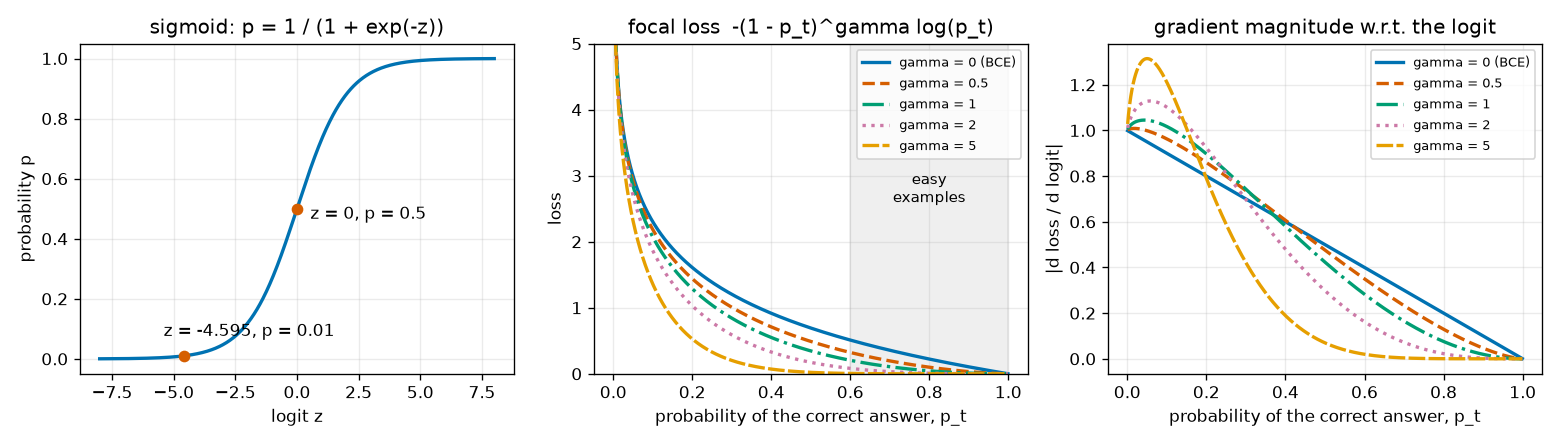
What to read from Figure 4-4:
- Left. The sigmoid passes through \(p = 0.5\) at \(z = 0\), and \(p = 0.01\) at \(z = -4.595\) (the value from the log-odds table).
- Middle. The solid blue line (\(\gamma = 0\)) is BCE. Even in the gray-shaded “easy cell” region (\(p_t \gt 0.6\)), BCE leaves a nonzero loss. As \(\gamma\) increases, the curve hugs the floor on the right. This is the same plot as Figure 1 of the paper.
- Right. The magnitude of the gradient with respect to the logit. For BCE it is the straight line \(1 - p_t\), and for \(\gamma = 2\) it is nearly 0 for \(p_t \gt 0.6\). Easy cells produce not only almost no loss but also almost no gradient. Meanwhile, for \(p_t\) below 0.2, the curves with \(\gamma \gt 0\) lie slightly above BCE. Focal loss does not cut down every cell; it shifts the weight of the loss toward the hard cells.
Returning to the 24,000-cell example, let's compute how the share of the loss changes depending on how easy the negative cells are (how low their \(p\) is). The focal loss uses \(\alpha = 0.25\), \(\gamma = 2\).
# 질의 300개 × 클래스 80개 = 24,000칸, 객체 10개. 양성은 아직 어려워 p = 0.3, 음성은 쉬워서 p = p_neg 라고 하자.
cells, num_pos = 300 * 80, 10
num_neg = cells - num_pos
print("  24,000칸 · 양성 10칸(p=0.3) · 음성 23,990칸(p=p_neg) 의 손실 합")
print("  p_neg   BCE: 양성 합  음성 합  음성 몫 |  포컬: 양성 합  음성 합  음성 몫")
for p_neg in [0.1, 0.05, 0.02, 0.01]:
    zp = torch.logit(torch.tensor(0.3, dtype=torch.float64))
    zn = torch.logit(torch.tensor(p_neg, dtype=torch.float64))
    one, zero = torch.tensor(1.0, dtype=torch.float64), torch.tensor(0.0, dtype=torch.float64)
    bce_pos = num_pos * bce_with_logits(zp, one).item()
    bce_neg = num_neg * bce_with_logits(zn, zero).item()
    fl_pos = num_pos * focal_loss_elementwise(zp, one).item()
    fl_neg = num_neg * focal_loss_elementwise(zn, zero).item()
    print(f"  {p_neg:<5}   {bce_pos:9.2f}  {bce_neg:8.2f}  {100 * bce_neg / (bce_pos + bce_neg):5.1f}%  |"
          f"  {fl_pos:10.3f}  {fl_neg:8.3f}  {100 * fl_neg / (fl_pos + fl_neg):5.1f}%")
  24,000칸 · 양성 10칸(p=0.3) · 음성 23,990칸(p=p_neg) 의 손실 합
  p_neg   BCE: 양성 합  음성 합  음성 몫 |  포컬: 양성 합  음성 합  음성 몫
  0.1         12.04   2527.60   99.5%  |       1.475    18.957   92.8%
  0.05        12.04   1230.53   99.0%  |       1.475     2.307   61.0%
  0.02        12.04    484.66   97.6%  |       1.475     0.145    9.0%
  0.01        12.04    241.11   95.2%  |       1.475     0.018    1.2%
With BCE, the negatives account for 95% of the total loss no matter how easy they get (\(p = 0.01\)). With focal loss, their share drops quickly as the negatives get easier: 9.0% at \(p = 0.02\) and 1.2% at \(p = 0.01\). However, when the negatives are less easy (\(p = 0.1\)), they still make up 92.8% even with focal loss. What focal loss removes is the “easy” negatives, not all negatives.
Why is α 0.25 for positives?
To fix the imbalance, it seems we should give the rare positives a larger weight, yet \(\alpha = 0.25\) multiplies positives by 0.25 and negatives by 0.75. It looks backward. The last row of the table above shows why. The \(\gamma = 2\) modulating factor cuts the easy negatives down so hard that now the positives account for most of the loss (98.8%). \(\alpha\) is a knob that pulls that skew back a little. The paper also notes that “as \(\gamma\) is increased, \(\alpha\) should be decreased slightly”, and says the two values must be chosen together. The defaults in RF-DETR's code are also \(\alpha = 0.25\), \(\gamma = 2\).
The gradient of focal loss
The gradient of BCE was \(p - y\). The gradient of focal loss is obtained the same way (differentiate with respect to \(p\) first, then multiply by \(p(1 - p)\)). Start with a positive cell (\(y = 1\), \(p_t = p\)).
- Positive cell — differentiating \(\mathrm{FL} = -\alpha\,(1 - p)^{\gamma}\log p\) with respect to the logit
- \(\frac{\partial\, \mathrm{FL}}{\partial p} = -\alpha\left[\, \frac{d}{dp}(1 - p)^{\gamma} \cdot \log p + (1 - p)^{\gamma} \cdot \frac{d}{dp}\log p \,\right]\)
- Product rule \((fg)' = f'g + fg'\), with \(f = (1 - p)^\gamma\) and \(g = \log p\).
- \(\frac{d}{dp}(1 - p)^\gamma = \gamma(1 - p)^{\gamma - 1} \cdot (-1)\) (chain rule: the derivative of the inner \(1 - p\) is \(-1\)), and \(\frac{d}{dp}\log p = \frac{1}{p}\).
- Multiply by the sigmoid's derivative \(p(1 - p)\). In the first term, \((1 - p)^{\gamma - 1} \cdot (1 - p) = (1 - p)^\gamma\) with a \(p\) left over; in the second term, \(p\) cancels and \((1 - p)^{\gamma} \cdot (1 - p) = (1 - p)^{\gamma + 1}\).
- Factor out \((1 - p)^\gamma\) and tidy up the signs: \(-\big[-\gamma p \log p + (1 - p)\big] = \gamma p\log p + p - 1\). Setting \(\gamma = 0\) gives \(\alpha(p - 1)\), i.e., the BCE gradient \(p - y\) multiplied by \(\alpha\).
For a negative cell (\(y = 0\)), \(\mathrm{FL} = -(1 - \alpha)\,p^{\gamma}\log(1 - p)\). Relative to the derivation above, the roles of \(p\) and \(1 - p\) are swapped (so the sign flips once when differentiating with respect to \(p\)) and \(\alpha\) becomes \(1 - \alpha\), so following the same computation gives
\(\frac{\partial\, \mathrm{FL}}{\partial z} = (1 - \alpha)\,p^{\gamma}\,\big(p - \gamma\,(1 - p)\log(1 - p)\big) \qquad (y = 0)\)
Written in one line using \(p_t\), the two cases are as follows (the sign is \(+\) for positives and \(-\) for negatives).
\(\frac{\partial\, \mathrm{FL}}{\partial z} = \pm\,\alpha_t\,(1 - p_t)^{\gamma}\,\big(\gamma\,p_t\log p_t + p_t - 1\big)\)
- Worked example — positive cell with \(z = 2\) (\(p = 0.8808\), predicted well), \(\alpha = 0.25\), \(\gamma = 2\)
- \((1 - p)^{2} = 0.1192^2 = 0.01421\)
- The modulating factor.
- \(\log 0.8808 = -0.1269\) is the value from the earlier BCE worked example.
- The BCE gradient for the same cell was \(p - y = -0.1192\). With focal loss it is about 1/98 of that. A well-predicted cell barely touches the network.
Implementing it in the same form as the official implementation
sigmoid_focal_loss in rfdetr/models/criterion.py of the official RF-DETR repository computes in the following order.
-
prob = inputs.sigmoid()— logits to probabilities. -
ce_loss = F.binary_cross_entropy_with_logits(inputs, targets, reduction="none")— the per-cell \(-\log p_t\) in numerically stable form. -
p_t = prob * targets + (1 - prob) * (1 - targets)— the probability on the correct side. -
loss = ce_loss * ((1 - p_t) ** gamma)— the modulating factor. - Multiply by
alpha_t = alpha * targets + (1 - alpha) * (1 - targets)(only whenalphais 0 or greater). - Return
loss.mean(1).sum() / num_boxes. The caller multiplies this by the number of queries, so in the end it is the sum over all cells divided by the number of positives (objects).
The sixth step is important. Averaging over all 24,000 cells would make the value vanishingly small because of the near-zero losses of the negative cells. So detectors divide the sum of the loss by the number of positives. The focal loss paper also states that it normalizes by “the number of assigned anchors”. The implementation below follows the same order but uses the bce_with_logits built in this chapter for the second step.
def focal_loss_elementwise(z: torch.Tensor, t: torch.Tensor, alpha: float = 0.25, gamma: float = 2.0) -> torch.Tensor:
    """원소마다의 포컬 손실 FL = −α_t · (1 − p_t)^γ · log(p_t). z: 로짓, t: 0/1 목표 (모양은 같고 무엇이든).

    공식 구현(rfdetr/models/criterion.py 의 sigmoid_focal_loss)과 같은 순서로 계산한다.
    """
    p = torch.sigmoid(z)
    ce = bce_with_logits(z, t)  # −log(p_t): 수치 안정 형태의 BCE 를 그대로 쓴다
    p_t = p * t + (1 - p) * (1 - t)  # 정답 쪽 확률: 양성이면 p, 음성이면 1 − p
    loss = ce * (1 - p_t) ** gamma  # 쉬운 칸(p_t 가 1 에 가까운 칸)의 손실을 줄이는 조절 인자
    if alpha >= 0:  # 음수를 주면 α 균형을 끈다
        alpha_t = alpha * t + (1 - alpha) * (1 - t)  # 양성이면 α, 음성이면 1 − α
        loss = alpha_t * loss
    return loss

def sigmoid_focal_loss(inputs: torch.Tensor, targets: torch.Tensor, num_boxes: float, alpha: float = 0.25,
                       gamma: float = 2.0) -> torch.Tensor:
    """모든 칸의 포컬 손실을 더해 양성(객체) 수로 나눈다.

    음성 칸까지 센 전체 칸 수로 나누면 값이 0 에 가까워져 버리므로, 양성 수로 나누는 것이 탐지기의 관례다.
    공식 구현은 (B, Q, K) 로짓에 대해 `loss.mean(1).sum() / num_boxes` 를 돌려주고 부르는 쪽에서 Q 를 곱한다.
    질의 축으로 평균 낸 뒤 Q 를 곱하면 합이므로, 결국 이 함수와 같은 값(전체 합 / num_boxes)이다.
    """
    return focal_loss_elementwise(inputs, targets, alpha, gamma).sum() / num_boxes
def focal_grad_formula(z: torch.Tensor, t: torch.Tensor, alpha: float = 0.25, gamma: float = 2.0) -> torch.Tensor:
    """본문에서 유도한 ∂FL/∂z = ± α_t · (1 − p_t)^γ · (γ · p_t · log p_t + p_t − 1). 부호는 양성 +, 음성 −."""
    p = torch.sigmoid(z)
    p_t = p * t + (1 - p) * (1 - t)
    alpha_t = alpha * t + (1 - alpha) * (1 - t)
    sign = 2 * t - 1  # 양성 +1, 음성 −1
    return sign * alpha_t * (1 - p_t) ** gamma * (gamma * p_t * torch.log(p_t) + p_t - 1)
torch.manual_seed(args.seed)
z = (torch.randn(4, 300, 80, dtype=torch.float64) * 3).requires_grad_(True)  # (B, Q, K) 로짓
t = (torch.rand(4, 300, 80) < 0.01).double()  # 양성 약 1%
p = torch.sigmoid(z.detach())
p_t = torch.where(t == 1, p, 1 - p)
alpha_t = torch.where(t == 1, torch.tensor(0.25, dtype=torch.float64), torch.tensor(0.75, dtype=torch.float64))
by_definition = -alpha_t * (1 - p_t) ** 2 * torch.log(p_t)  # 정의 FL = −α_t (1 − p_t)^γ log p_t 를 그대로
mine = focal_loss_elementwise(z, t, alpha=0.25, gamma=2.0)
print(f"  check: focal_loss_elementwise vs 정의식 최대 차이 {(mine - by_definition).abs().max().item():.1e}")
plain = focal_loss_elementwise(z, t, alpha=-1, gamma=0.0)  # γ = 0, α 균형 끔 → BCE 여야 한다
ref = F.binary_cross_entropy_with_logits(z, t, reduction="none")
print(f"  check: γ=0 · α 끔 → F.binary_cross_entropy_with_logits 와의 최대 차이 {(plain - ref).abs().max().item():.1e}")
mine.sum().backward()
diff = (z.grad - focal_grad_formula(z.detach(), t)).abs().max().item()
print(f"  check: autograd 기울기 vs 유도한 기울기 식 최대 차이 {diff:.1e}")
[5] 포컬 손실
  check: focal_loss_elementwise vs 정의식 최대 차이 4.1e-11
  check: γ=0 · α 끔 → F.binary_cross_entropy_with_logits 와의 최대 차이 8.9e-16
  check: autograd 기울기 vs 유도한 기울기 식 최대 차이 5.6e-16
  z=+0, y=1: p=0.5000  BCE=0.6931  FL=0.04332  ∂BCE/∂z=-0.5000  ∂FL/∂z=-0.07457
  z=+2, y=1: p=0.8808  BCE=0.1269  FL=0.00045  ∂BCE/∂z=-0.1192  ∂FL/∂z=-0.00122
  z=-2, y=0: p=0.1192  BCE=0.1269  FL=0.00135  ∂BCE/∂z=+0.1192  ∂FL/∂z=+0.00365
  z=+2, y=0: p=0.8808  BCE=2.1269  FL=1.23756  ∂BCE/∂z=+0.8808  ∂FL/∂z=+0.80754
What to check in the output:
- The implementation matches the defining formula \(-\alpha_t(1 - p_t)^\gamma\log p_t\), and with \(\gamma = 0\) and \(\alpha\) balancing turned off it matches PyTorch's BCE.
- The gradient computed by autograd matches the formula derived above to the \(10^{-16}\) level.
- The last four lines are the loss and gradient for four kinds of cells. The gradient of a well-predicted positive (\(z = +2\), \(y = 1\)) is \(-0.00122\), as in the worked example, and that of a well-predicted negative (\(z = -2\), \(y = 0\)) is \(+0.00365\), both far smaller than BCE's \(\pm 0.1192\); a badly wrong negative (\(z = +2\), \(y = 0\)) gets \(+0.80754\), not much different from BCE's \(0.8808\).
Where these formulas reappear in later chapters
- Matching cost in chapter 7 and chapter 11: the classification cost used when pairing predictions with ground truths has the form “focal loss treated as positive − focal loss treated as negative”.
- IA-BCE in chapter 9: the loss of a negative cell is \(p^2 \cdot \big(-\log(1 - p)\big)\), which is the negative side of focal loss (\(\gamma = 2\)) with only \(\alpha_t\) removed. The positive cells use the soft-target BCE seen earlier.
- RF-DETR's default setting is IA-BCE (
ia_bce_loss=True);sigmoid_focal_lossremains in the code as the loss used when that setting is turned off.
Prior-probability bias initialization
Imbalance also causes trouble the moment training starts. In a freshly built network, the last linear layer has weights that are small random numbers near 0 and biases near 0. Then the logits of all cells are near 0, and the probabilities near 0.5. Of 24,000 cells, 23,990 have the answer “no”, yet the network starts out answering “fifty-fifty” for every cell.
The focal loss paper's remedy is to change not the loss but the initialization. At the start of training, every cell is made to answer “the probability of being positive is about \(\pi\) (pi)”. \(\pi\) is a small value encoding the prior knowledge that positives are rare; the paper uses \(\pi = 0.01\). Here this is called prior-probability bias initialization.
- The bias that makes the initial prediction \(\pi\)
- \(z = w \cdot x + b \approx b\)
- The logit of the last linear layer. Before training, the weights \(w\) are small values near 0, so \(w \cdot x\) is small and the logit is determined almost entirely by the bias \(b\).
- We want the initial prediction to be \(\pi\).
- Use the inverse of the sigmoid (the log-odds). For \(\pi = 0.01\), \(b = -\log\frac{0.99}{0.01} = -\log 99 = -4.5951\).
Let's compute how much this bias changes the initial loss, using the 24,000-cell example (10 positives). The loss is the sum divided by the number of positives, 10.
- The loss at the moment training starts
- \(b = 0,\ \text{BCE}:\qquad \frac{24{,}000 \times (-\log 0.5)}{10} = \frac{24{,}000 \times 0.69315}{10} = 1663.55\)
- Every cell has \(p = 0.5\), so each cell, positive or negative, contributes \(-\log 0.5 = 0.69315\).
- Every cell has \(p = 0.01\). The positive cells are badly wrong at \(-\log 0.01 = 4.6052\), while the negative cells are almost right at \(-\log 0.99 = 0.01005\). The initial loss drops to 1/58.
- Even with focal loss (\(\alpha = 0.25\), \(\gamma = 2\)), at \(p = 0.5\) the modulating factor is only \(0.25\), so the negative cells dominate the loss.
- With focal loss and the prior bias, the summed loss of the 23,990 negative cells is 0.02, effectively gone, and nearly all of the loss comes from the 10 positive cells. The loss of a single positive cell, \(0.25 \times 0.9801 \times 4.6052 = 1.13\), is the total loss as is.
def prior_bias(prior_prob: float = 0.01) -> float:
    """σ(b) = π 가 되는 편향 b = −log((1 − π) / π). π = 0.01 이면 −4.5951."""
    return -math.log((1 - prior_prob) / prior_prob)
# 학습을 시작하는 순간의 손실: 24,000칸 모두 같은 확률을 낸다고 보고, 양성 수(10)로 나눈 값
print(f"  사전 확률 편향: π=0.01 → b={prior_bias(0.01):.4f}, σ(b)={torch.sigmoid(torch.tensor(prior_bias(0.01))).item():.4f}")
targets = torch.zeros(300, 80, dtype=torch.float64)
targets[:num_pos, 0] = 1.0  # 양성 10칸
for name, bias in [("b = 0 (p = 0.5)       ", 0.0), ("b = −4.5951 (p = 0.01)", prior_bias(0.01))]:
    logits = torch.full((300, 80), bias, dtype=torch.float64)
    bce = bce_with_logits(logits, targets).sum().item() / num_pos
    focal = sigmoid_focal_loss(logits, targets, num_pos).item()
    print(f"  초기 손실 {name}: BCE {bce:9.2f}   포컬 {focal:8.3f}")
  사전 확률 편향: π=0.01 → b=-4.5951, σ(b)=0.0100
  초기 손실 b = 0 (p = 0.5)       : BCE   1663.55   포컬  311.830
  초기 손실 b = −4.5951 (p = 0.01): BCE     28.72   포컬    1.130
With the bias left at 0, the loss at the first step is in the hundreds to thousands, and most of it is the signal “pull the probabilities of the negative cells down from 0.5”. A large loss produces large gradients, and the first few steps shake not only the last layer but the layers below it as well. The paper reports that training with ordinary cross-entropy without this initialization quickly diverged, and that initializing with \(\pi = 0.01\) alone was enough to make training work (Section 5.1). It also notes that the results were insensitive to the exact value of \(\pi\).
RF-DETR's public code (rfdetr/models/lwdetr.py) performs exactly this initialization right after creating the classification head.
# init prior_prob setting for focal loss
prior_prob = 0.01
bias_value = -math.log((1 - prior_prob) / prior_prob)
self.class_embed.bias.data = torch.ones(num_classes) * bias_value
class_embed is the classification head (nn.Linear), and its bias is filled with \(-4.5951\) for every class. The experiment at the end of this chapter directly compares training with and without this initialization.
Normalization layers and residual connections
When layers are stacked deep, the magnitude of the values grows or shrinks erratically from layer to layer, and training becomes unstable. A normalization layer rescales intermediate values back to “mean 0, variance 1”. The variants differ in which numbers are grouped together for averaging; the computation is the same in all of them. Compute the mean \(\mu\) (mu) and variance \(s^2\) of the group, then convert
\(\hat{x} = \frac{x - \mu}{\sqrt{s^2 + \epsilon}}, \qquad \text{출력} = a\,\hat{x} + c\)
and output \(a\,\hat{x} + c\). \(\epsilon\) is a small number that prevents division by zero (PyTorch default \(10^{-5}\)), and \(a\) (scale) and \(c\) (shift) are learned parameters that start at \(a = 1\), \(c = 0\). They let the network recover the scale and location that normalization erased, if it needs them.
A note on symbols
Papers and the PyTorch documentation write the scale and shift parameters as \(\gamma\) and \(\beta\). This chapter has already used \(\gamma\) for focal loss and \(\beta\) for Adam, so they are written \(a\) and \(c\) here (in PyTorch they are named weight and bias). Variance is also usually written \(\sigma^2\), but \(\sigma\) is already the sigmoid, so it is written \(s^2\).
Batch normalization
Batch normalization (BatchNorm; Ioffe & Szegedy, 2015) groups one feature (channel) across the whole batch. If the input is (B, C) and \(x_{ij}\) is the \(j\)-th feature of the \(i\)-th sample, then for each feature \(j\) it computes
\(\mu_j = \frac{1}{B}\sum_{i=1}^{B} x_{ij}, \qquad s_j^2 = \frac{1}{B}\sum_{i=1}^{B} (x_{ij} - \mu_j)^2\)
The axis being averaged over is the batch axis. For a feature map (B, C, H, W), the batch and spatial axes (B, H, W) are grouped together for each channel (nn.BatchNorm2d).
Layer normalization
Layer normalization (LayerNorm; Ba et al., 2016) groups the features of a single sample. For each sample \(i\) it computes
\(\mu_i = \frac{1}{C}\sum_{j=1}^{C} x_{ij}, \qquad s_i^2 = \frac{1}{C}\sum_{j=1}^{C} (x_{ij} - \mu_i)^2\)
The axis being averaged over is the feature axis, and the other samples in the batch are not looked at at all. For a Transformer token sequence (B, N, D), the \(D\) numbers of one token form a group (chapter 5).
Figure 4-5 in the original shows, side by side, the groups over which the two normalizations compute their mean and variance for an input (B, C) (rows are samples 1 … \(B\), columns are features \(j = 1 \dots C\)). Batch normalization groups one column (the \(B\) values of one feature), so its output depends on the values of other samples. Layer normalization groups one row (the \(C\) features of one sample), so it is independent of other samples.
- Worked example — normalizing an input with 2 samples and 3 features both ways (\(\epsilon\) ignored)
- \(x = \begin{pmatrix} 1 & 2 & 3 \\ 3 & 6 & 9 \end{pmatrix} \qquad (B = 2,\ C = 3)\)
- The second sample is 3 times the first.
- Batch normalization, per column. The first column \((1, 3)\) has mean 2 and variance \(\frac{(1-2)^2 + (3-2)^2}{2} = 1\). The second column \((2, 6)\) has mean 4 and variance \(\frac{4 + 4}{2} = 4\). The third column \((3, 9)\) has mean 6 and variance 9.
- The batch-normalized output: (value − mean) ÷ standard deviation for each column. Every column now has mean 0 and variance 1. The first sample's outputs are all \(-1\), which means “smaller than the second sample”; had the second sample been different, the output would have been different too.
- Layer normalization, per row. The first row \((1, 2, 3)\) has mean 2 and variance \(\frac{1 + 0 + 1}{3} = \frac{2}{3}\). The second row \((3, 6, 9)\) has mean 6 and variance \(\frac{9 + 0 + 9}{3} = 6\).
- The layer-normalized output, with \(\sqrt{2/3} = 0.8165\) and \(\sqrt{6} = 2.4495\). The two rows are now identical. Layer normalization erases each sample's overall scale (the factor of 3) and keeps only “the relative shape among the features”. The other row was not used in computing either row.
x = torch.tensor([[1.0, 2.0, 3.0], [3.0, 6.0, 9.0]])  # (B=2, C=3): 그림 두 장, 특징 세 개

# 배치 정규화: 특징(열)마다, 배치 축(dim=0)으로 평균 · 분산
mu_b, var_b = x.mean(dim=0), x.var(dim=0, unbiased=False)  # (3,), (3,)
bn_manual = (x - mu_b) / torch.sqrt(var_b + 1e-5)

# 층 정규화: 표본(행)마다, 특징 축(dim=1)으로 평균 · 분산
mu_l, var_l = x.mean(dim=1, keepdim=True), x.var(dim=1, unbiased=False, keepdim=True)  # (2, 1), (2, 1)
ln_manual = (x - mu_l) / torch.sqrt(var_l + 1e-5)

bn, ln = nn.BatchNorm1d(3), nn.LayerNorm(3)  # 처음에는 크기 조절 1, 이동 0 → 정규화만 한다
bn.train()
print(f"  check: 배치 정규화 손계산 vs nn.BatchNorm1d 최대 차이 {(bn(x) - bn_manual).abs().max().item():.1e}")
print(f"  check: 층 정규화 손계산 vs nn.LayerNorm 최대 차이 {(ln(x) - ln_manual).abs().max().item():.1e}")
[6] 배치 정규화 · 층 정규화
  check: 배치 정규화 손계산 vs nn.BatchNorm1d 최대 차이 6.0e-08
  check: 층 정규화 손계산 vs nn.LayerNorm 최대 차이 0.0e+00
  배치 평균 [2.0, 4.0, 6.0] 배치 분산 [1.0, 4.0, 9.0]
  배치 정규화 출력 [[-1.0, -1.0, -1.0], [1.0, 1.0, 1.0]]
  행 평균 [2.0, 6.0] 행 분산 [0.6667, 6.0]
  층 정규화 출력   [[-1.2247, 0.0, 1.2247], [-1.2247, 0.0, 1.2247]]
  이동 평균 [0.2, 0.4, 0.6] 이동 분산 [1.1, 1.7, 2.7]
  추론 모드 출력   [[0.7628, 1.2271, 1.4606], [2.6697, 4.295, 5.1121]]
Training mode and inference mode
Batch normalization is awkward at inference time. If only a single image is fed in, “the batch mean” is just that image itself. So batch normalization operates in two ways.
- Training mode (
model.train()): normalize with the mean and variance of the current batch, and blend those values a little at a time into a running average that is kept for later. The PyTorch default is (new value) = 0.9 × (old value) + 0.1 × (this batch's value). - Inference mode (
model.eval()): normalize with the stored running mean and running variance. The result does not depend on what else is in the batch.
In the output above, the “running mean [0.2, 0.4, 0.6]” is the initial value 0 blended with 10% of the batch mean \((2, 4, 6)\): \(0.9 \times 0 + 0.1 \times (2, 4, 6)\). The “running variance [1.1, 1.7, 2.7]” is the initial value 1 blended with 10% of the batch variance, but for the running variance PyTorch uses the variance divided by \(B - 1\) instead of \(B\), i.e., \((2, 8, 18)\): \(0.9 \times 1 + 0.1 \times 2 = 1.1\). The first value in inference mode is \((1 - 0.2)/\sqrt{1.1} = 0.7628\), completely different from the \(-1\) in training mode. Layer normalization behaves the same in both modes. Forgetting model.eval() before evaluation is a common mistake with models that contain batch normalization, and the shape classification experiment later shows its effect in numbers.
Batch normalization wobbles when the batch is small
The mean and variance in batch normalization are estimates measured on the batch. The mean of \(B\) samples varies each time the samples are drawn, and that wobble (standard deviation) is roughly proportional to \(1/\sqrt{B}\). With a batch of 64 images the statistics are stable, but with 2 they wobble \(\sqrt{64 / 2} = 5.66\) times more. The same image then produces different outputs depending on which other images came with it, and that noise interferes with training. Let's measure it directly on a feature map (512, 8, 6, 6) obtained by passing 512 shapes-world images through a fixed random convolution that produces 8 features per 16×16 patch.
# 도형 세상 그림을 고정된 무작위 합성곱(16×16 패치마다 특징 8개)에 통과시킨 특징 맵으로 통계의 흔들림을 잰다
dataset = ShapesDataset(n_images, seed=0)
torch.manual_seed(args.seed)
conv = nn.Conv2d(3, 8, kernel_size=16, stride=16)
with torch.no_grad():
    feats = torch.relu(conv(dataset.images.float() / 255.0))  # (n, 8, 6, 6)
pop_mean = feats.mean(dim=(0, 2, 3))  # (8,) 전체 데이터에서의 채널 평균: 배치 통계가 맞혀야 할 값
pop_std = feats.std(dim=(0, 2, 3))
probe = feats[0]  # 늘 배치의 첫 자리에 넣을 그림 한 장 (8, 6, 6)
generator = torch.Generator().manual_seed(args.seed)
results = {}
for batch_size in [2, 4, 16, 64]:
    means, stds, bn_out, ln_out = [], [], [], []
    for _ in range(n_batches):
        batch = feats[torch.randint(0, len(feats), (batch_size,), generator=generator)]  # 무작위 배치 (B, 8, 6, 6)
        means.append(batch.mean(dim=(0, 2, 3)))  # 배치 정규화가 쓰는 통계: 채널마다 (B, H, W) 축 평균
        stds.append(batch.std(dim=(0, 2, 3), unbiased=False))
        batch = torch.cat([probe[None], batch[1:]])  # 첫 자리를 probe 로 바꾼 배치: 함께 들어간 그림만 매번 다르다
        mu, sd = batch.mean(dim=(0, 2, 3)), batch.std(dim=(0, 2, 3), unbiased=False)
        bn_out.append((probe - mu[:, None, None]) / (sd[:, None, None] + 1e-5))  # probe 의 배치 정규화 출력
        # 층 정규화(RF-DETR 프로젝터 방식): 위치마다 채널 축(dim=0)으로 평균 · 분산 → 다른 그림과 무관
        ln_out.append((probe - probe.mean(dim=0)) / (probe.std(dim=0, unbiased=False) + 1e-5))
    means, stds = torch.stack(means), torch.stack(stds)  # (n_batches, 8)
    results[batch_size] = {
        "mean_wobble": (means.std(dim=0) / pop_std).mean().item(),  # 배치 평균의 흔들림 (전체 표준편차 단위)
        "std_wobble": (stds.std(dim=0) / pop_std).mean().item(),  # 배치 표준편차의 흔들림
        "bn_out_wobble": torch.stack(bn_out).std(dim=0).mean().item(),  # 같은 그림의 출력이 배치마다 달라지는 정도
        "ln_out_wobble": torch.stack(ln_out).std(dim=0).mean().item(),
        "means_ch0": (means[:, 0] - pop_mean[0]) / pop_std[0],
    }
  특징 맵 (512, 8, 6, 6), 배치 300개씩
  배치 크기  배치 평균의 흔들림  배치 표준편차의 흔들림  같은 그림의 출력 흔들림(BN)  (LN)
       2            0.1475              0.3966                0.1159    0.0000
       4            0.1014              0.3181                0.1031    0.0000
      16            0.0516              0.2037                0.0577    0.0000
      64            0.0256              0.1094                0.0277    0.0000
  배치 2 와 64 의 평균 흔들림 비 5.77 (√(64/2) = 5.66)
- Figure: Figure 4-6 Left: batch means of channel 0 measured over 300 random batches (on a scale set by the mean and standard deviation of the full data). Right: how much the normalized output of the same single image varies from batch to batch.
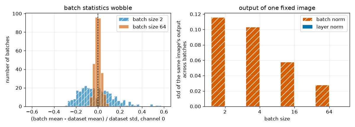
Reading the table and Figure 4-6:
- Batch statistics wobble depending on the batch size. The wobble of the batch mean (on a scale where the full data's standard deviation is 1) is 0.1475 for batch size 2 and 0.0256 for batch size 64. The ratio is 5.77, nearly the expected \(\sqrt{32} = 5.66\). In the left panel, the batch-2 means spread from roughly \(-0.3\) to \(0.6\), while the batch-64 means cluster tightly around 0. The batch standard deviation wobbles in the same way (0.3966 versus 0.1094).
- That wobble carries over into the output. The variation (standard deviation) across batches of the batch-normalized output for the same single image is 0.1159 for batch size 2 and 0.0277 for batch size 64. Since the normalized output has a standard deviation of about 1, with batch size 2 noise of roughly 12% of that size is added to the output depending on “which images came along with it” (the hatched bars in the right panel).
- The output wobble of layer normalization is exactly 0. It never looks at other images, so whether the batch size is 1 or 64, the same image produces the same output.
Why RF-DETR replaced batch normalization in the projector with layer normalization
The LW-DETR projector (chapter 9) uses batch normalization after its convolutions. RF-DETR replaced it with layer normalization. The paper gives the reason as “to enable training on consumer-grade GPUs with gradient accumulation” (Section 3). Gradient accumulation collects the gradients of several small batches (4 images by default in the public code) and applies them in a single update (chapter 11). Gradients can be accumulated that way, but batch normalization statistics are computed during the forward pass from the images actually fed in together, so accumulation cannot stabilize them. Layer normalization does not depend on the batch size. The paper states that this replacement lowers COCO performance but is necessary for training on consumer hardware (in the ablation discussion in Section 4).
The layer normalization in RF-DETR's projector normalizes the \(C\) channel values at each position of the feature map (B, C, H, W) as one group (LayerNorm in the public code's projector.py: moves the channel axis to the end and applies F.layer_norm). The layer normalization in the experiment above works the same way.
Residual connections
A residual connection (skip connection; He et al., 2016, ResNet) adds a layer's input directly to its output. If the layer's computation is \(f\),
\(x_{\text{out}} = x + f(x)\)
The layer only has to learn “the difference to add to the input (the residual)” rather than “the entire new value”. The more important effect shows up in backpropagation.
- Residual connections give the gradient a “shortcut” (the single-number case)
- \(\frac{\partial x_{\text{out}}}{\partial x} = 1 + f'(x)\)
- Differentiate \(x + f(x)\) with respect to \(x\). The leading 1 is the term that comes from the added input.
- \(D\) layers without residual connections: by the chain rule, the per-layer derivatives are multiplied together. If they are all 0.5, for example, 20 layers give \(0.5^{20} = 9.5 \times 10^{-7}\). The gradient vanishes before it reaches the first layer (the vanishing gradient problem).
- \(D\) layers with residual connections: when expanded, there is a 1 at the front. It is the path that follows only the “added input” route at every layer. No matter how small the \(f_l'\) are, this 1 remains, so the gradient reaches the first layer intact.
def first_layer_gradient(depth: int, residual: bool, width: int = 64, seed: int = 0) -> float:
    """깊이 depth 인 MLP 에서, 출력의 합을 첫 층 입력으로 미분한 기울기의 크기(노름).

    residual=False: x ← tanh(Linear(x))          (층을 그냥 쌓음)
    residual=True : x ← x + tanh(Linear(x))      (잔차 연결)
    """
    torch.manual_seed(seed)
    layers = [nn.Linear(width, width) for _ in range(depth)]
    x0 = torch.randn(16, width, requires_grad=True)  # (16, width)
    x = x0
    for layer in layers:
        fx = torch.tanh(layer(x))
        x = x + fx if residual else fx
    x.sum().backward()
    return x0.grad.norm().item()
[7] 잔차 연결과 기울기
  층 수   그냥 쌓음       잔차 연결
     1      1.814e+01      3.521e+01
     5      1.241e+00      4.798e+01
    10      8.286e-02      7.069e+01
    20      4.599e-04      9.779e+01
    40      1.274e-09      2.647e+02
This is the magnitude of the gradient of the output sum with respect to the input, for layers of width 64 stacked with tanh. Plain stacking makes it vanish: \(4.6 \times 10^{-4}\) at 20 layers and \(1.3 \times 10^{-9}\) at 40 layers. With residual connections, the gradient is still alive even at 40 layers (it actually grows slightly as the network gets deeper, and normalization layers are what keep that in check). The Transformer block in chapter 5 wraps both attention and the FFN in “residual connection + layer normalization”. Both the 12-layer ViT backbone and the decoder can be trained thanks to this structure.
Convolution basics
Convolution is the layer that handles images. In RF-DETR it is used in the first layer that splits the image into patches (chapter 6) and in the projector (chapter 9). Here only what later chapters need is briefly summarized. Numerical examples of convolution and a more detailed explanation are in “Convolutional neural networks: networks that read images” in chapter 4 of the World Model tutorial.
Kernel, stride, padding, and output size
A convolution slides a small plate of weights over the input and, at each position of the plate, outputs one value: “the sum of the products of the overlapping numbers”. Three numbers determine the shape.
- Kernel (filter): the sliding plate of weights. Its side length is written \(F\) (\(F = 3\) for 3×3). It uses the same weights at every position, so it has few parameters.
- Stride \(S\): how many cells to move at a time. With \(S = 2\), the output's width and height are halved.
- Padding \(P\): how many rows of zeros to add around the edge of the input. It lets the kernel be placed at the edges too.
For an input of side length \(n_{\text{in}}\), the output size \(n_{\text{out}}\) is:
\(n_{\text{out}} = \left\lfloor \frac{n_{\text{in}} - F + 2P}{S} \right\rfloor + 1\)
Within the padded length \(n_{\text{in}} + 2P\), a kernel of length \(F\) can travel a distance of \(n_{\text{in}} + 2P - F\); moving \(S\) cells at a time, it can move \(\lfloor \cdot / S \rfloor\) times, and adding 1 counts the starting position.
- Worked example — three convolutions on a 96×96 image
- \(F = 3,\ S = 1,\ P = 1:\qquad \left\lfloor \frac{96 - 3 + 2}{1} \right\rfloor + 1 = 95 + 1 = 96\)
- A 3×3 kernel with padding 1 preserves the size. This is the most common setting.
- Stride 2 halves the size. This is the setting the RF-DETR projector uses to halve a feature map.
- When the kernel size equals the stride, the kernels do not overlap and are laid out like tiles. A 96×96 image becomes 6×6 = 36 cells.
Including channels, a convolution layer maps (B, C_in, H, W) → (B, C_out, H', W'), and its parameters are \(C_{\text{out}} \times C_{\text{in}} \times F \times F\) weights and \(C_{\text{out}}\) biases. A 3×3 convolution from 3 channels to 8 channels has \(8 \times 3 \times 3 \times 3 + 8 = 224\).
def conv_out(n_in: int, kernel: int, stride: int = 1, padding: int = 0) -> int:
    """출력 크기 = ⌊(n_in − F + 2P) / S⌋ + 1."""
    return (n_in - kernel + 2 * padding) // stride + 1

x = torch.randn(2, 3, 96, 96)  # (B, C, H, W): 도형 세상 그림 두 장
for kernel, stride, padding in [(3, 1, 1), (3, 2, 1), (1, 1, 0), (16, 16, 0)]:
    conv = nn.Conv2d(3, 8, kernel_size=kernel, stride=stride, padding=padding)
    n_params = sum(p.numel() for p in conv.parameters())
    print(f"  커널 {kernel:>2} · 스트라이드 {stride:>2} · 패딩 {padding}: 공식 {conv_out(96, kernel, stride, padding):>2} → 실제 {tuple(conv(x).shape)}, 매개변수 {n_params}")
up = nn.ConvTranspose2d(8, 8, kernel_size=2, stride=2)  # 전치 합성곱: (n − 1)·S − 2P + F = 2n
print(f"  전치 합성곱 커널 2 · 스트라이드 2: {tuple(torch.randn(2, 8, 6, 6).shape)} → {tuple(up(torch.randn(2, 8, 6, 6)).shape)}")
1×1 convolution and patchification
Two special cases come up often in later chapters.
- A 1×1 convolution (pointwise convolution) (\(F = 1\)) does not look at neighbors at all. It is a linear layer whose weights are shared by all positions, turning \(C_{\text{in}}\) numbers into \(C_{\text{out}}\) numbers at each position. It is used to change the number of channels (the projector's C2f) or to produce classification logits at each position (the experiment at the end of this chapter).
- A convolution with stride equal to kernel size is the same as “cutting the image into non-overlapping \(F \times F\) pieces and applying the same linear layer to each piece”. These pieces are called patches, and the ViT in chapter 6 turns an image into a token sequence with a single such convolution. RF-DETR (nano) splits a 384×384 image into 16×16 patches, so \(384 / 16 = 24\), giving \(24 \times 24 = 576\) tokens.
# 스트라이드 = 커널 = 16 인 합성곱은 "16×16 패치로 자르고, 패치마다 같은 선형 층" 과 같다
conv = nn.Conv2d(3, 8, kernel_size=16, stride=16)
by_conv = conv(x)  # (2, 8, 6, 6)
patches = x.reshape(2, 3, 6, 16, 6, 16).permute(0, 2, 4, 1, 3, 5).reshape(2, 36, 3 * 16 * 16)  # (2, 36, 768)
linear_w = conv.weight.reshape(8, 3 * 16 * 16)  # 커널을 펴면 선형 층의 가중치 (8, 768)
by_linear = patches @ linear_w.T + conv.bias  # (2, 36, 8): 패치 36개 각각에 같은 선형 층
by_linear = by_linear.reshape(2, 6, 6, 8).permute(0, 3, 1, 2)  # (2, 8, 6, 6) 으로 되돌려 비교
print(f"  check: 패치 나누기 + 선형 층 vs 합성곱(커널 16 · 스트라이드 16) 최대 차이 {(by_conv - by_linear).abs().max().item():.1e}")
[8] 합성곱 출력 크기 · 패치 나누기
  커널  3 · 스트라이드  1 · 패딩 1: 공식 96 → 실제 (2, 8, 96, 96), 매개변수 224
  커널  3 · 스트라이드  2 · 패딩 1: 공식 48 → 실제 (2, 8, 48, 48), 매개변수 224
  커널  1 · 스트라이드  1 · 패딩 0: 공식 96 → 실제 (2, 8, 96, 96), 매개변수 32
  커널 16 · 스트라이드 16 · 패딩 0: 공식  6 → 실제 (2, 8, 6, 6), 매개변수 6152
  전치 합성곱 커널 2 · 스트라이드 2: (2, 8, 6, 6) → (2, 8, 12, 12)
  check: 패치 나누기 + 선형 층 vs 합성곱(커널 16 · 스트라이드 16) 최대 차이 1.1e-06
  check: 1×1 합성곱 vs 위치마다의 선형 층 최대 차이 2.4e-07
The output sizes from the formula match the actual shapes, and the parameter count matches the worked example (224). The last two lines confirm the two claims above: the output of the convolution (kernel 16, stride 16) matches “cut into patches and apply a linear layer”, and the output of the 1×1 convolution matches “a linear layer at each position”, to within rounding error (\(10^{-6}\) – \(10^{-7}\), float32).
Transposed convolution
If convolution shrinks a feature map, transposed convolution enlarges it. Each number of the input stamps a kernel-sized imprint onto the output, and overlapping regions are summed. The output size, inverting the convolution formula, is \(n_{\text{out}} = (n_{\text{in}} - 1)\,S - 2P + F\). With \(F = 2\), \(S = 2\), \(P = 0\), it is \((n_{\text{in}} - 1) \cdot 2 + 2 = 2\,n_{\text{in}}\), exactly double (6 → 12 in the output above). The RF-DETR projector uses this setting (ConvTranspose2d(kernel_size=2, stride=2)) to double the size of a feature map.
Minimal PyTorch
Reading tensor shapes
All data in PyTorch is a tensor (an array of numbers with multiple axes), and the list of lengths along each axis is its shape. Most errors in deep learning code come from mismatched shapes, so this tutorial writes the shape in a comment wherever it changes. Shapes that come up often:
| What | Shape | Meaning of the axes |
| Image batch | | Batch, color channel (RGB), height, width |
| Feature map | | Batch, channel, height, width (input and output of convolutions) |
| Token sequence | | Batch, number of tokens, dimension of one token (input and output of a Transformer, chapter 5) |
| Classification logits | | Batch, number of queries, number of classes (detector output, chapter 7) |
| Boxes | | Batch, number of queries, (cx, cy, w, h) (chapter 2) |
nn.Module and the five-step training loop
A neural network is built as a class that inherits from nn.Module. Layers (parameters) are created in __init__, and the forward pass is written in forward. Backpropagation is handled by autograd. As an example, here is a small CNN (convolutional neural network) that looks at a 96×96 image containing a single shape and tells whether it is a circle, a square, or a triangle. It contains every component covered in this chapter (convolution, batch normalization, ReLU, linear layer, softmax cross-entropy, AdamW).
class ShapeClassifier(nn.Module):
    """도형 하나가 그려진 그림 (B, 3, 96, 96) → 클래스 로짓 (B, 3).

    [합성곱 → 배치 정규화 → ReLU] 를 세 번(매번 가로 · 세로 절반), 전체 평균, 선형 층.
    """

    def __init__(self, num_classes: int = NUM_CLASSES, width: int = 16):
        super().__init__()
        chans = [3, width, 2 * width, 4 * width]
        blocks = []
        for c_in, c_out in zip(chans[:-1], chans[1:]):
            blocks += [nn.Conv2d(c_in, c_out, 3, stride=2, padding=1), nn.BatchNorm2d(c_out), nn.ReLU()]
        self.features = nn.Sequential(*blocks)  # (B, 3, 96, 96) → (B, 64, 12, 12)
        self.classifier = nn.Linear(chans[-1], num_classes)

    def forward(self, images: torch.Tensor) -> torch.Tensor:
        feature_map = self.features(images)  # (B, 64, 12, 12)
        pooled = feature_map.mean(dim=(2, 3))  # (B, 64): 위치 축 평균(전역 평균 풀링)
        return self.classifier(pooled)  # (B, 3) 로짓 — 소프트맥스는 손실 함수 안에서 한다
Training always repeats the same five steps. All training code in this tutorial is built on this skeleton.
-
optimizer.zero_grad()— clear the gradients from the previous step (because PyTorch accumulates gradients instead of overwriting them). -
logits = model(x)— the forward pass. -
loss = …— compute the loss. -
loss.backward()— backpropagation. The.gradof every parameter is filled in. -
optimizer.step()— the optimizer looks at the gradients and updates the parameters.
torch.manual_seed(args.seed)
model = ShapeClassifier().to(device)
optimizer = torch.optim.AdamW(model.parameters(), lr=1e-3, weight_decay=1e-4)
batch_size = 64
history = []
for epoch in range(1, epochs + 1):
    model.train()  # 학습 모드: 배치 정규화가 배치 통계를 쓰고 이동 통계를 갱신한다
    order = torch.randperm(len(train_x), device=device)
    total = 0.0
    for start in range(0, len(order), batch_size):
        index = order[start:start + batch_size]
        optimizer.zero_grad()  # ① 지난 스텝의 기울기를 지운다
        logits = model(train_x[index])  # ② 순전파: (B, 3, 96, 96) → (B, 3)
        loss = F.cross_entropy(logits, train_y[index])  # ③ 손실: 소프트맥스 교차 엔트로피(배치 평균)
        loss.backward()  # ④ 역전파: 모든 매개변수의 .grad 를 채운다
        optimizer.step()  # ⑤ 갱신: θ ← θ − (AdamW 가 정한 양)
        total += loss.item() * len(index)
    model.eval()  # 추론 모드: 배치 정규화가 이동 통계를 쓴다
    with torch.no_grad():  # 평가에는 기울기가 필요 없다
        val_logits = model(val_x)
        val_loss = F.cross_entropy(val_logits, val_y).item()
        val_acc = (val_logits.argmax(dim=1) == val_y).float().mean().item()
    history.append((total / len(train_x), val_loss, val_acc))
    print(f"  에폭 {epoch:>2}: 학습 손실 {history[-1][0]:.4f}  검증 손실 {val_loss:.4f}  검증 정확도 {100 * val_acc:.1f}%")
[10] 도형 분류 CNN: 학습 고리 5단계
  학습 (1500, 3, 96, 96) · 검증 (500, 3, 96, 96), 클래스별 학습 그림 수 [508, 508, 484]
  에폭  1: 학습 손실 1.0374  검증 손실 1.0607  검증 정확도 42.2%
  에폭  2: 학습 손실 0.9444  검증 손실 0.9748  검증 정확도 61.4%
  에폭  3: 학습 손실 0.7705  검증 손실 0.7514  검증 정확도 67.2%
  에폭  4: 학습 손실 0.5817  검증 손실 0.5064  검증 정확도 97.8%
  에폭  5: 학습 손실 0.4259  검증 손실 0.3701  검증 정확도 99.8%
  에폭  6: 학습 손실 0.3077  검증 손실 0.2723  검증 정확도 99.2%
  에폭  7: 학습 손실 0.2336  검증 손실 0.2046  검증 정확도 100.0%
  에폭  8: 학습 손실 0.1783  검증 손실 0.1609  검증 정확도 100.0%
  혼동 행렬 (행 = 정답, 열 = 예측; 원 · 사각형 · 삼각형)
    [160, 0, 0]
    [0, 172, 0]
    [0, 0, 168]
  매개변수 24,003개, 마지막 검증 정확도 100.0% (500/500)
  (참고) model.train() 인 채로 2장씩 넣어 평가하면 검증 정확도 74.8%
  그림 저장: ch04-shape-cnn.png
- Figure: Figure 4-7 Training curves of the shape classification CNN (left) and its predictions on 8 validation images (right; each title shows the predicted class and its probability).
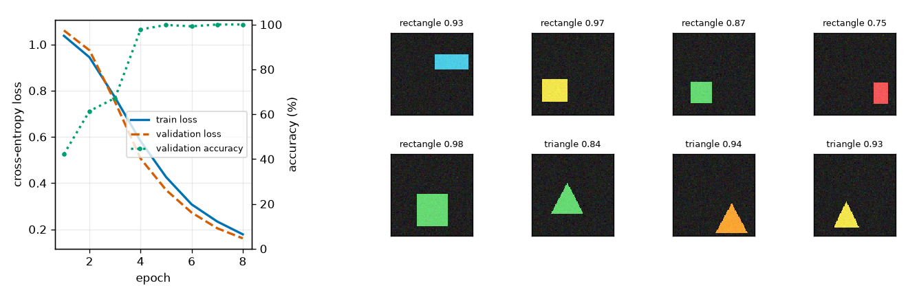
Reading the results:
- After 8 epochs the validation accuracy is 100.0% (500 out of 500), and every off-diagonal entry of the confusion matrix is 0. Classifying images that contain a single shape is an easy problem for which a CNN with 24,003 parameters is enough.
- In the left panel of Figure 4-7, the training and validation losses go down together (there is no sign of overfitting, where only the validation loss climbs back up). Accuracy stays at 42–67% through epoch 3 and then jumps to 97.8% at epoch 4.
- All eight predictions on the right are correct, with probabilities of 0.75–0.98. Since the model was trained with softmax cross-entropy, the probabilities of the three classes sum to 1.
- The last line is a concrete case of the “Training mode and inference mode” box. Evaluating the same model while still in
model.train(), feeding 2 images at a time, drops the accuracy to 74.8%. This is because batch normalization normalizes with the statistics of those 2 images instead of the running statistics stored during training. Callingmodel.eval()before evaluation is not optional.
Experiment: three ways to train an imbalanced classifier
Let's check in the shapes world what difference the formulas in this chapter make in actual training. It is still too early to build a whole detector (chapter 7), so we set up a problem with the same character as a detector's classification output.
Task: finding the cells that contain shape centers
Divide a 96×96 image into a 12×12 grid (each cell is 8×8 pixels), and for each cell and each class ask “does the center of a shape of this class lie in this cell?”. Each image has \(3 \times 12 \times 12 = 432\) cells, and the only positives are the shapes in the image (1–4).
def center_targets(dataset: ShapesDataset, grid: int = GRID) -> torch.Tensor:
    """그림마다 (클래스 3, 격자 12, 격자 12) 의 0/1 목표. "클래스 k 인 도형의 중심이 이 칸에 있는가".

    한 그림의 칸은 3 × 12 × 12 = 432개이고 양성은 도형 수(1 – 4개)뿐이다 → 양성 약 0.6%.
    """
    targets = torch.zeros(len(dataset), NUM_CLASSES, grid, grid)
    for i, target in enumerate(dataset.targets):
        for (cx, cy, _w, _h), cls in zip(target["boxes"].tolist(), target["labels"].tolist()):
            col, row = min(int(cx * grid), grid - 1), min(int(cy * grid), grid - 1)  # 중심이 떨어지는 칸
            targets[i, cls, row, col] = 1.0
    return targets
The model is a small CNN made of five convolution layers and a 1×1 convolution head. An independent sigmoid is applied to each cell of the output (B, 3, 12, 12). Think of it as a scaled-down version of a detector's classification output (B, Q, K) in which the query slots are replaced by grid cells.
class CenterGridNet(nn.Module):
    """그림 (B, 3, 96, 96) → 칸마다 · 클래스마다의 로짓 (B, 3, 12, 12). 클래스마다 독립인 시그모이드를 쓴다.

    prior_prob 을 주면 마지막 층의 편향을 b = −log((1 − π)/π) 로 둔다 (RF-DETR 의 class_embed 와 같은 초기화).
    주지 않으면 PyTorch 의 기본 초기화(0 근처의 작은 값)를 그대로 쓴다 → 처음 예측이 0.5 근처.
    """

    def __init__(self, num_classes: int = NUM_CLASSES, width: int = 32, prior_prob: float | None = None):
        super().__init__()
        self.body = nn.Sequential(
            nn.Conv2d(3, width, 3, stride=2, padding=1), nn.ReLU(),  # (B, 32, 48, 48)
            nn.Conv2d(width, 2 * width, 3, stride=2, padding=1), nn.ReLU(),  # (B, 64, 24, 24)
            nn.Conv2d(2 * width, 2 * width, 3, stride=2, padding=1), nn.ReLU(),  # (B, 64, 12, 12)
            nn.Conv2d(2 * width, 2 * width, 3, padding=1), nn.ReLU(),  # 12×12 를 유지하며 주변을 더 본다
            nn.Conv2d(2 * width, 2 * width, 3, padding=1), nn.ReLU(),
        )
        self.head = nn.Conv2d(2 * width, num_classes, kernel_size=1)  # 1×1 합성곱 = 칸마다의 선형 분류 머리
        if prior_prob is not None:
            nn.init.constant_(self.head.bias, prior_bias(prior_prob))

    def forward(self, images: torch.Tensor) -> torch.Tensor:
        return self.head(self.body(images))
Three settings are compared.
| Setting | Loss | Last-layer bias | Initial prediction |
| (a) BCE + default bias | BCE | PyTorch default initialization (near 0) | Every cell near 0.5 |
| (b) BCE + prior-probability bias | BCE | \(-4.5951\) (\(\pi = 0.01\)) | Every cell near 0.01 |
| (c) Focal + prior-probability bias | Focal loss (\(\alpha = 0.25\), \(\gamma = 2\)) | \(-4.5951\) (\(\pi = 0.01\)) | Every cell near 0.01 |
All other conditions are identical.
- Data: 2,000 training images (seed 0), 500 validation images (seed 1). Batch size 32.
- Loss scale: in all three settings, the sum of the losses over all cells in the batch is divided by the number of positives in that batch (the same as the official implementation).
- Optimizer: AdamW (learning rate \(10^{-3}\), weight decay \(10^{-4}\)) for 30 epochs. A separate 12-epoch run with SGD (learning rate 0.01, momentum 0.9), the optimizer used in the focal loss paper, checks early-training stability.
- For the same seed, the initial weights of the body and the batch order are the same across settings. The runs are repeated with 3 seeds (0, 1, 2) to get the mean and standard deviation.
The metrics are measured by flattening all cells of the validation data (500 × 432 = 216,000 cells) into one list.
- Positive recall and precision (chapter 3): computed by treating cells with probability at or above a threshold of 0.5 as “cells predicted positive”.
- AP (chapter 3): list the cells in descending order of probability, record the precision so far each time a positive cell appears, and average those values. It is a metric that requires no threshold.
- Mean \(p\): the average predicted probability over all cells. It is compared with the actual positive rate.
@torch.no_grad()
def cell_metrics(logits: torch.Tensor, targets: torch.Tensor, threshold: float = 0.5) -> dict:
    """모든 칸을 한 줄로 펴서 잰 양성 재현율 · 정밀도(문턱값 0.5)와 평균 정밀도(AP, 문턱값과 무관).

    AP: 칸을 점수가 높은 순으로 늘어놓고, 양성 칸이 나올 때마다 그때까지의 정밀도를 적어 평균 낸 값.
    """
    scores, labels = torch.sigmoid(logits).flatten(), targets.flatten() > 0.5
    predicted = scores >= threshold
    tp = (predicted & labels).sum().item()
    order = scores.argsort(descending=True)
    hits = labels[order].double()
    precision_at = hits.cumsum(0) / torch.arange(1, len(hits) + 1, device=hits.device)
    return {
        "recall": tp / max(labels.sum().item(), 1),
        "precision": tp / max(predicted.sum().item(), 1),
        "ap": ((precision_at * hits).sum() / hits.sum()).item(),
        "mean_p": scores.mean().item(),
    }
def train_center(train_x, train_t, val_x, val_t, loss_name: str, prior_prob, optimizer_name: str, epochs: int,
                 seed: int, batch_size: int = 32) -> dict:
    """설정 하나를 학습한다. 돌려주는 값: 스텝마다의 손실, 에폭마다의 검증 지표(0번은 학습 전), 모델."""
    torch.manual_seed(seed)  # 설정이 달라도 몸통의 초기 가중치와 배치 순서는 같다
    model = CenterGridNet(prior_prob=prior_prob).to(train_x.device)
    if optimizer_name == "adamw":
        optimizer = torch.optim.AdamW(model.parameters(), lr=1e-3, weight_decay=1e-4)
    else:
        optimizer = torch.optim.SGD(model.parameters(), lr=0.01, momentum=0.9, weight_decay=1e-4)

    def loss_fn(logits, targets):
        num_pos = targets.sum().clamp(min=1.0)  # 이 배치의 양성(도형) 수
        if loss_name == "bce":
            return bce_with_logits(logits, targets).sum() / num_pos
        return sigmoid_focal_loss(logits, targets, num_pos, alpha=0.25, gamma=2.0)

    def evaluate():
        model.eval()
        with torch.no_grad():
            logits = torch.cat([model(val_x[i:i + 256]) for i in range(0, len(val_x), 256)])
        model.train()
        return cell_metrics(logits, val_t)

    losses, history, diverged = [], [evaluate()], False
    generator = torch.Generator().manual_seed(seed)
    for _epoch in range(epochs):
        order = torch.randperm(len(train_x), generator=generator).to(train_x.device)
        for start in range(0, len(order) - batch_size + 1, batch_size):
            index = order[start:start + batch_size]
            optimizer.zero_grad()  # ① 기울기 비우기
            logits = model(train_x[index])  # ② 순전파 (B, 3, 12, 12)
            loss = loss_fn(logits, train_t[index])  # ③ 손실
            if not torch.isfinite(loss):
                diverged = True
                break
            loss.backward()  # ④ 역전파
            optimizer.step()  # ⑤ 매개변수 갱신
            losses.append(loss.item())
        if diverged:
            break
        history.append(evaluate())
    return {"losses": losses, "history": history, "model": model, "diverged": diverged}
Results
This is the [9] part of the run output. For each optimizer there are three tables (early training, final epoch, AP per epoch), and at the end there is a table with varying thresholds.
[9] 불균형 실험: 도형 중심이 있는 칸 찾기
  학습 2000장 · 검증 500장, 목표 모양 (2000, 3, 12, 12), 그림당 칸 432개
  양성 칸: 학습 4995개 / 864000칸 = 0.578% (그림당 평균 2.50개)
  모델 매개변수 130,371개, 배치 32 (에폭당 62 스텝), 시드 [0, 1, 2]
  ── 옵티마이저 AdamW (lr 1e-3), 30 에폭, 시드 3개 평균
  설정                         처음 평균 p | 손실: 1스텝째  10스텝째  100스텝째 | 1에폭 뒤: 평균 p    AP
  (a) BCE + 기본 편향            0.4991   |       121.03     18.73       4.75  |        0.0071  0.016
  (b) BCE + 사전 확률 편향       0.0101   |         6.36      5.45       2.32  |        0.0060  0.341
  (c) 포컬 + 사전 확률 편향      0.0101   |         1.13      0.56       0.45  |        0.0597  0.048
  마지막 에폭(30)의 검증 지표 (평균±표준편차)   평균 p     재현율         정밀도         AP          발산
  (a) BCE + 기본 편향                         0.0057   0.829±0.027   0.872±0.014   0.928±0.010   0/3
  (b) BCE + 사전 확률 편향                    0.0057   0.834±0.017   0.862±0.020   0.928±0.010   0/3
  (c) 포컬 + 사전 확률 편향                   0.0105   0.710±0.030   0.923±0.006   0.914±0.005   0/3
  에폭별 검증 AP                       1       2       4       8      12      20      30
  (a) BCE + 기본 편향             0.016   0.132   0.504   0.813   0.878   0.918   0.928
  (b) BCE + 사전 확률 편향        0.341   0.599   0.807   0.888   0.917   0.929   0.928
  (c) 포컬 + 사전 확률 편향       0.048   0.074   0.295   0.641   0.819   0.889   0.914
  ── 옵티마이저 SGD (lr 0.01, 모멘텀 0.9), 12 에폭, 시드 3개 평균
  설정                         처음 평균 p | 손실: 1스텝째  10스텝째  100스텝째 | 1에폭 뒤: 평균 p    AP
  (a) BCE + 기본 편향            0.4991   |       121.03      9.18       5.54  |        0.0071  0.039
  (b) BCE + 사전 확률 편향       0.0101   |         6.36      6.22       5.15  |        0.0047  0.100
  (c) 포컬 + 사전 확률 편향      0.0101   |         1.13      1.12       0.56  |        0.0358  0.031
  마지막 에폭(12)의 검증 지표 (평균±표준편차)   평균 p     재현율         정밀도         AP          발산
  (a) BCE + 기본 편향                         0.0049   0.445±0.320   0.750±0.136   0.661±0.270   0/3
  (b) BCE + 사전 확률 편향                    0.0060   0.783±0.027   0.839±0.032   0.891±0.030   0/3
  (c) 포컬 + 사전 확률 편향                   0.0301   0.284±0.101   0.875±0.028   0.714±0.009   0/3
  에폭별 검증 AP                       1       2       4       8      12
  (a) BCE + 기본 편향             0.039   0.077   0.217   0.424   0.661
  (b) BCE + 사전 확률 편향        0.100   0.183   0.531   0.822   0.891
  (c) 포컬 + 사전 확률 편향       0.031   0.062   0.209   0.511   0.714
  ── 문턱값에 따른 검증 재현율 · 정밀도 (AdamW, 첫 시드, 마지막 에폭)
  (a) BCE + 기본 편향          문턱 0.3: 0.907 · 0.820   문턱 0.5: 0.866 · 0.864   문턱 0.7: 0.809 · 0.899   | 양성 칸의 확률 중앙값 0.991
  (b) BCE + 사전 확률 편향     문턱 0.3: 0.859 · 0.853   문턱 0.5: 0.823 · 0.885   문턱 0.7: 0.784 · 0.912   | 양성 칸의 확률 중앙값 0.996
  (c) 포컬 + 사전 확률 편향    문턱 0.3: 0.900 · 0.765   문턱 0.5: 0.742 · 0.915   문턱 0.7: 0.513 · 0.979   | 양성 칸의 확률 중앙값 0.709
  그림 저장: ch04-centers.png
  그림 저장: ch04-imbalance.png
- Figure: Figure 4-8 Top: 4 validation images and their positive cells (green squares; the text beside each is the class: cir circle, rec square, tri triangle). Bottom: the probabilities predicted by the model trained with setting (c) (seed 0), drawn as the maximum over the three classes for each cell. The white markers are the ground-truth cells.
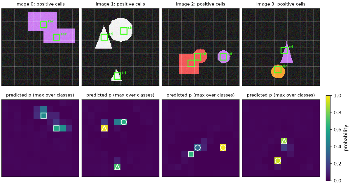
The top row of Figure 4-8 shows the task: of the 144 cells, there are only as many green squares as there are shapes. In the bottom row, the model gives probabilities near 0 to most cells and high probabilities to the ground-truth cells and the cells right next to them. When a center lies close to a cell boundary, confusing it with the neighboring cell is the main error in this task (which is why AP does not reach 1).
- Figure: Figure 4-9 Top row AdamW (30 epochs), bottom row SGD (12 epochs). Left: training loss over the first 150 steps (both axes on a log scale). Middle: validation positive recall (threshold 0.5). Right: validation AP. Lines are the mean over 3 seeds, and the light bands span the minimum to maximum. Solid line (a), dashed line (b), dash-dotted line (c).
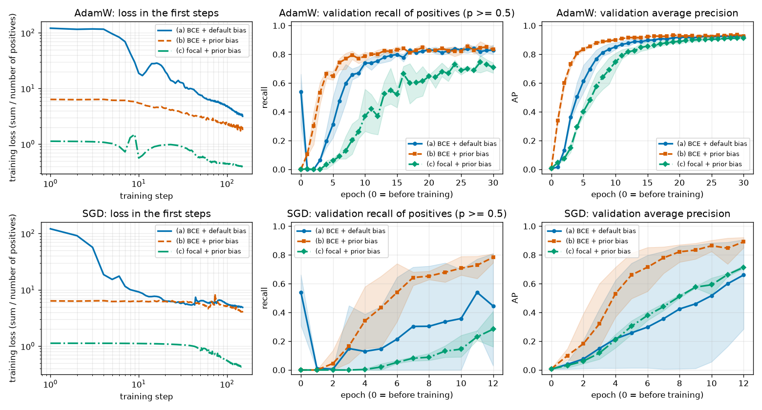
Reading the results: prior-probability bias
The first loss matches the calculation. Computing by hand with 432 cells per image and 2.5 positives on average gives the following, which matches the step-1 loss column of the output.
| Setting | Hand calculation | Actual first loss |
| (a) | \(432 \times 0.6931 / 2.5 = 119.8\) | 121.03 (slightly different because the initial prediction is not exactly 0.5) |
| (b) | \((2.5 \times 4.6052 + 429.5 \times 0.01005) / 2.5 = 6.33\) | 6.36 |
| (c) | \(0.25 \times 0.99^2 \times 4.6052 = 1.13\) (the negatives' share is negligibly small) | 1.13 |
(a) spends its first few dozen steps “pulling the negative cells down”.
- In the top left of Figure 4-9, the loss of (a) starts at 121 and drops steeply to 18.73 at step 10 and 4.75 at step 100. All it learns in this stretch is the fact that “almost every cell is negative”, which a single bias can express. (b) starts out already knowing that.
- That difference shows up directly in early performance. Validation AP after 1 epoch is 0.016 for (a) and 0.341 for (b), and after 4 epochs it is 0.504 versus 0.807.
- In the middle panel, the epoch-0 recall of (a) being near 0.5 is not real performance. Every cell's probability is near 0.5, so about half of them happen to cross the threshold by chance; after 1 epoch it drops to 0.
With AdamW, (a) eventually catches up. At 20 epochs it is 0.918 versus 0.929, and at 30 epochs both are \(0.928 \pm 0.010\). Adam erases the magnitude of the gradient, so whether the first loss is 121 or 6, each step moves by a similar amount, and a large initial loss does not wreck training.
With SGD, the difference is much larger. SGD moves in proportion to the gradient, so a large initial loss translates directly into large updates.
- After 12 epochs, validation AP is \(0.661 \pm 0.270\) for (a) and \(0.891 \pm 0.030\) for (b). Not only is (a)'s mean lower, but its results vary widely from seed to seed (the wide blue band in the bottom row of Figure 4-9).
- In this experiment there was never any divergence where the loss became
nan(the divergence column shows 0/3). The divergence reported in the focal loss paper happened in a much larger and deeper detector (RetinaNet) with about 100,000 locations. Here, instead of “divergence”, it showed up as “slow training that varies erratically with the seed”.
Reading the results: why focal loss did not win
In this experiment, focal loss (c) did not beat BCE (b). The results, as they are:
| AdamW, validation | (b) BCE + prior-probability bias | (c) Focal + prior-probability bias |
| AP after 4 epochs | 0.807 | 0.295 |
| AP after 12 epochs | 0.917 | 0.819 |
| AP after 30 epochs | \(0.928 \pm 0.010\) | \(0.914 \pm 0.005\) |
| Recall (threshold 0.5) after 30 epochs | \(0.834 \pm 0.017\) | \(0.710 \pm 0.030\) |
| Precision (threshold 0.5) after 30 epochs | \(0.862 \pm 0.020\) | \(0.923 \pm 0.006\) |
| Median probability of positive cells (seed 0) | 0.996 | 0.709 |
Focal loss learned more slowly; after 30 epochs its AP had caught up to within 0.014 (not a large gap, given a standard deviation across seeds of 0.005–0.010), but its recall at threshold 0.5 was clearly lower. With SGD too, it trailed after 12 epochs with an AP of 0.714 versus 0.891. The reasons break down into three.
① Focal loss does not push probabilities all the way up to 1.
- Once a positive cell's probability reaches about 0.7, the modulating factor \((1 - 0.7)^2 = 0.09\) cuts that cell's loss to about 1/11. There is little reason left to push it higher. That is why the median probability of positive cells is 0.996 for BCE and 0.709 for focal loss.
- Most of the difference in recall comes from this. Lowering the threshold to 0.3 raises focal loss's recall to 0.900, higher than BCE's 0.859 (at the cost of lower precision, 0.765 versus 0.853), while at threshold 0.7 it plunges to 0.513. The last table of the output shows this.
- Measured by the threshold-independent AP, the two models' “ability to rank” is nearly the same. A model trained with focal loss produces lower probabilities, so its threshold should not be set to the same value as for a BCE model.
- Mean \(p\) tells the same story. The actual positive rate is 0.58%; after 30 epochs, BCE's mean \(p\) is 0.0057, matching that rate (the probabilities are well calibrated), while focal loss's is 0.0105, almost double. Focal loss also cares little about pulling the probabilities of easy negative cells all the way down to 0.
② Focal loss gets off to a slow start. At the moment training starts, with every cell at \(p = 0.01\), compare the force with which the 429.5 negative cells of one image push “down” against the force with which the 2.5 positive cells push “up” (the sum of the gradients with respect to the logits).
- Worked example — gradients at the moment training starts (\(p = 0.01\))
- \(\text{BCE:}\quad \text{음성 한 칸 } p - 0 = 0.01, \qquad \text{양성 한 칸 } p - 1 = -0.99\)
- BCE, per cell: 0.01 for a negative cell and \(-0.99\) for a positive cell, since the BCE gradient is \(p - y\).
- BCE, per image: 4.30 pushing down versus 2.48 pushing up. The negative and positive sides oppose each other with similar strength. From the very start, a signal flows that distinguishes “which cells are positive”.
- Focal loss, one negative cell: the gradient formula for negative cells derived earlier. \(-2 \times 0.99 \times \log 0.99 = 0.0199\). Because of the modulating factor \(p^2 = 10^{-4}\), it is about 1/4,500 of BCE's.
- Focal loss, one positive cell. \(2 \times 0.01 \times \log 0.01 = -0.0921\).
- Focal loss, per image: 0.00096 pushing down versus 0.66 pushing up. “Down” is about 1/700 of “up”. The negative cells put up almost no resistance.
So when training starts with focal loss, the network first raises the probabilities of all cells together (the easiest move, requiring only a larger bias). Only after the negative cells' probabilities have risen enough for the modulating factor to grow does resistance from the negative side appear, and only then does the network start telling positives from negatives. The output bears traces of this: after 1 epoch, mean \(p\) is 0.0060 for (b) but 0.0597 for (c), ten times the actual positive rate. The subsequent AP curve (top right of Figure 4-9) trails (b) by several epochs.
③ This task has little of the ailment that focal loss treats.
- Positives to negatives is about 1 : 172, with 432 cells per image. What the focal loss paper targeted was about 100,000 locations per image and an imbalance on the order of 1 : 1000.
- Most negative cells in the shapes world are plain dark background and very easy. The BCE in (b) brings mean \(p\) close to the actual positive rate (0.0060) within 1 epoch, and after that the summed loss of the negative cells no longer gets in the way of training. The situation assumed in the earlier 24,000-cell calculation, where “the summed loss of easy negatives overwhelms the positives”, does not last long in this small task.
- That leaves focal loss with little to gain from its benefit (removing easy negatives) and only its costs (the low probabilities of ① and the slow start of ②).
What this experiment can and cannot tell us
- The experiments in this tutorial use a small CNN, 2,000 images, and a single set of hyperparameters per setting (\(\alpha = 0.25\), \(\gamma = 2\), fixed learning rate). The learning rate and \(\alpha\) were not tuned separately for focal loss.
- The focal loss paper reports that when training RetinaNet on COCO, focal loss with \(\gamma = 2\) achieved 2.9 higher AP than cross-entropy with only \(\alpha\) balancing (Section 5.1). These two results come from completely different conditions, so they do not contradict each other.
- The takeaway is neither “focal loss is always better” nor “focal loss is useless”. Focal loss is a remedy for the ailment where easy negatives are so overwhelmingly numerous that their summed loss dominates training, and when the ailment is mild, the remedy has little effect. Prior-probability bias initialization, on the other hand, works cheaply and reliably whatever the loss.
The IA-BCE used by RF-DETR (chapter 9) connects with both observations from this experiment. For negative cells it uses the same modulating factor \(p^2\) as focal loss to remove easy negatives, but for positive cells it uses soft-target BCE without a modulating factor, so that the score rises all the way to the target (how well the box fits).
Summary
- A neural network is a function with parameters \(\theta\). A linear layer \(h = Wx + b\) maps the last axis \(n \to m\) and has \(mn + m\) parameters. Activation functions: ReLU (decoder FFN), GELU (ViT), SiLU (projector).
- Training is \(\theta \leftarrow \theta - \eta\nabla_\theta L\). Backpropagation is the chain rule, passing (incoming gradient) × (local derivative) backward from the loss, and autograd does it for you.
- Adam erases the magnitude of the gradient and keeps its direction. AdamW places weight decay outside that division and shrinks the weights separately: \(\theta \leftarrow (1 - \eta\lambda)\theta\).
- Sigmoid \(\sigma(z) = 1/(1 + e^{-z})\): \(\sigma(-z) = 1 - \sigma(z)\), \(\sigma' = \sigma(1 - \sigma)\), and the logit \(z = \log\frac{p}{1 - p}\) is the log-odds.
- BCE \(= -y\log p - (1 - y)\log(1 - p)\) is the negative log of the Bernoulli likelihood. Its gradient with respect to the logit is \(p - y\). Compute it directly from the logit: \(\max(z, 0) - zy + \log(1 + e^{-|z|})\). With a soft target \(t\), the minimum is at \(p = t\).
- DETR uses softmax + a background class; Deformable DETR onward and RF-DETR use per-class sigmoids. “Nothing” means all class probabilities are low.
- Focal loss \(\mathrm{FL} = -\alpha_t(1 - p_t)^\gamma\log p_t\) cuts down the loss of well-predicted cells (1/100 for \(\gamma = 2\), \(p_t = 0.9\)). With \(\gamma = 0\) it is BCE. The loss is the sum divided by the number of positives.
- Prior-probability bias initialization \(b = -\log\frac{1 - \pi}{\pi}\) (\(-4.5951\) for \(\pi = 0.01\)) sets the initial prediction to \(\pi\) and greatly reduces the initial loss. RF-DETR's classification head is initialized this way.
- Batch normalization averages over the batch axis, layer normalization over the feature axis. With small batches, batch normalization statistics wobble in proportion to \(1/\sqrt{B}\). A residual connection \(x + f(x)\) adds 1 to the derivative, creating a shortcut for the gradient.
- The output size of a convolution is \(\lfloor (n_{\text{in}} - F + 2P)/S \rfloor + 1\). A convolution with stride equal to kernel size is patchification + a linear layer.
- In this tutorial's imbalance experiment, the prior-probability bias clearly helped early training (especially with SGD), while focal loss learned more slowly than BCE and reached a similar AP after 30 epochs (0.914 versus 0.928).
We now have the “general-purpose” components needed to build a detector. But the core of RF-DETR is not convolution; it is attention. The backbone, the decoder, and the way each prediction slot decides where in the image to look all rest on attention. Chapter 5 starts by computing attention by hand with a few numbers, then assembles this chapter's linear layers, softmax, layer normalization, and residual connections into a Transformer block.
Review questions
- 1. If a tensor of shape
(2, 300, 256)is fed intonn.Linear(256, 4), what is the output shape? How many parameters does this layer have? - A linear layer changes only the last axis, so the output is
(2, 300, 4). The parameters are \(4 \times 256 = 1024\) weights and 4 biases, 1,028 in total. (This is the shape of a layer that outputs 4 box coordinates for each of 300 queries.) - 2. In the 2-layer network from the text, if \(b_1 = 0.1\) is changed to \(b_1 = -1.5\) (keeping \(x = 2\), \(w_1 = 0.5\), \(w_2 = -1.5\), \(b_2 = 0.2\), \(y = 1\)), what is \(\frac{\partial L}{\partial w_1}\)?
- Since \(u = 0.5 \cdot 2 - 1.5 = -0.5 \lt 0\), \(h = \max(0, -0.5) = 0\), \(\hat{y} = -1.5 \cdot 0 + 0.2 = 0.2\), and \(L = (0.2 - 1)^2 = 0.64\). In backpropagation, \(\frac{\partial L}{\partial \hat{y}} = -1.6\) and \(\frac{\partial L}{\partial h} = -1.6 \times (-1.5) = 2.4\) are nonzero, but the ReLU derivative is 0 (\(u \lt 0\)), so \(\frac{\partial L}{\partial u} = 0\) and \(\frac{\partial L}{\partial w_1} = 0 \cdot x = 0\). Layer 1 learns nothing from this input.
- 3. A cell has logit \(z = -1\) (\(\sigma(-1) = 0.2689\)). (1) Find the BCE and the gradient with respect to the logit when the answer is \(y = 1\). (2) Compute the same loss in the numerically stable form and check that the values agree.
- (1) \(\operatorname{BCE} = -\log 0.2689 = 1.3133\). The gradient is \(p - y = 0.2689 - 1 = -0.7311\) (increase the logit). (2) \(\max(-1, 0) - (-1)(1) + \log(1 + e^{-|-1|}) = 0 + 1 + \log(1.3679) = 1 + 0.3133 = 1.3133\). They agree.
- 4. A positive cell is trained with soft-target BCE with target \(t = 0.8\). If the current prediction is \(p = 0.5\), what is the gradient with respect to the logit, and where does \(p\) go once training has converged? What is the loss then?
- The gradient is \(p - t = 0.5 - 0.8 = -0.3\) (increase the logit). The minimum is at \(p = t = 0.8\), where the loss is \(-0.8\log 0.8 - 0.2\log 0.2 = 0.1785 + 0.3219 = 0.5004\). It is not 0.
- 5. The model assigns \(p = 0.1\) to a negative cell (\(y = 0\)). Compute the focal loss with \(\alpha = 0.25\), \(\gamma = 2\) and the BCE, and find what fraction of the BCE the focal loss is.
- \(p_t = 1 - p = 0.9\). BCE \(= -\log 0.9 = 0.10536\). For focal loss, \(\alpha_t = 1 - \alpha = 0.75\) and the modulating factor is \((1 - 0.9)^2 = 0.01\), so \(0.75 \times 0.01 \times 0.10536 = 0.00079\). That is \(1 / (0.75 \times 0.01) \approx 1/133\) of the BCE (1/100 from the modulating factor, then another factor of 0.75 from \(\alpha_t\)).
- 6. If the prior probability is set to \(\pi = 0.05\), what should the last layer's bias be initialized to? With 1,000 cells of which 5 are positive, compare the initial BCE loss (sum ÷ number of positives) under this initialization with that for a bias of 0.
- \(b = -\log\frac{0.95}{0.05} = -\log 19 = -2.944\). Bias 0: \(1000 \times 0.6931 / 5 = 138.6\). Bias \(-2.944\): positives \(5 \times (-\log 0.05) = 5 \times 2.9957 = 14.98\), negatives \(995 \times (-\log 0.95) = 995 \times 0.05129 = 51.04\), total \(66.02 / 5 = 13.2\). About 1/10.
- 7. Normalize the first sample of the input \(x = \begin{pmatrix} 0 & 4 \\ 2 & 8 \end{pmatrix}\) (2 samples, 2 features) with batch normalization and with layer normalization (\(\epsilon\) ignored, \(a = 1\), \(c = 0\)).
- Batch normalization (per column): the first column \((0, 2)\) has mean 1 and variance 1 → \((0 - 1)/1 = -1\). The second column \((4, 8)\) has mean 6 and variance 4 → \((4 - 6)/2 = -1\). The first sample becomes \((-1, -1)\). Layer normalization (per row): the first row \((0, 4)\) has mean 2 and variance 4 → \(\big((0 - 2)/2,\ (4 - 2)/2\big) = (-1, 1)\). This answer does not change no matter what the second sample is.
- 8. RF-DETR (small) splits a 512×512 image into 16×16 patches. (1) If patchification is done with a convolution, what are the kernel, stride, and padding? (2) How many tokens result? (3) If a transposed convolution with kernel 2 and stride 2 is applied to that feature map, what is its side length?
- (1) Kernel 16, stride 16, padding 0. (2) \(\lfloor (512 - 16)/16 \rfloor + 1 = 31 + 1 = 32\), so \(32 \times 32 = 1024\) tokens. (3) \((32 - 1) \times 2 + 2 = 64\).
See also
Favorite site
- 04. Deep Learning Basics and Classification Loss
- ch04_basics.py - practice code for this chapter
- World Model tutorial, chapter 4: Deep Learning and PyTorch Basics
- Adam: A Method for Stochastic Optimization (Kingma & Ba, 2015)
- Decoupled Weight Decay Regularization (AdamW; Loshchilov & Hutter, 2019)
- Focal Loss for Dense Object Detection (Lin et al., 2017)
- Batch Normalization (Ioffe & Szegedy, 2015)
- Layer Normalization (Ba et al., 2016)
- Deep Residual Learning for Image Recognition (ResNet; He et al., 2016)
- End-to-End Object Detection with Transformers (DETR)
- Deformable DETR
- RF-DETR paper