RF-DETR:Tutorial:03-EvaluationMAP
lastmod 2026-11-18created 2026-11-182 edits
Scoring detectors: AP and mAP is chapter 3 of the RF-DETR tutorial. The abstract of the RF-DETR paper states that "RF-DETR (nano) achieves 48.0 AP on COCO," and the goal of this chapter is to understand that one sentence completely. Starting from what it means for a single predicted box to be "correct," it works through precision and recall, the curve that connects them, and AP, which reduces that curve to a single number, calculating each by hand and checking it in code. It uses the IoU from chapter 2 as the scoring criterion, and at the end it implements NMS, which removes overlapping predictions, laying the groundwork for understanding why the DETR family in chapter 7 can do without it.
- Original: 03. Scoring Detectors: AP and mAP (about 80 minutes to read, difficulty ★★☆☆☆)
- Practice code:
code/ch03_metrics.py. It contains matching (match_detections), the PR curve and 101-point AP, dataset scoring withevaluate_ap, the fake-detector experiments, and NMS. There is no training, so it finishes in a little over a minute on a CPU (--quickuses 60 images and takes 10–20 seconds). - Previous: 02. Boxes and IoU / Next: 04. Deep Learning Basics and Classification Loss
In this chapter you will learn:
- Why "accuracy" as used in classification is useless for detection
- The rules for matching predicted boxes to ground-truth boxes to sort out true positives (TP), false positives (FP), and false negatives (FN), and why duplicate predictions are penalized
- Precision and recall, the trade-off when moving the score threshold, and the precision–recall (PR) curve
- Computing AP by hand using PR curve interpolation and COCO's 101-point method
- mAP, and what each of COCO's AP, AP50, AP75, APS, APM, and APL measures
- Using fake-detector experiments to see how AP responds to box accuracy, score order, duplicate predictions, and junk predictions
- The NMS algorithm and its weaknesses, and what it means that the DETR family does not use NMS
Why "accuracy" doesn't work
When it comes to scoring a model, the first thing that comes to mind is accuracy. In a classification problem where you look at an image and decide "cat or dog," getting 93 of 100 images right means 93% accuracy.
\(\text{accuracy} = \frac{\text{number of correct answers}}{\text{total number of questions}}\)
For this formula to work, you have to be able to count the "questions." In classification, one image is one question, with one answer. But as chapter 1 showed, the answer in object detection is not a single item but a set. A detector looks at an image and outputs any number of the following.
- Box: a rectangle enclosing the object (\((c_x, c_y, w, h)\) or \((x_0, y_0, x_1, y_1)\) from chapter 2)
- Class: what the object is (in the shapes world: circle, rectangle, or triangle)
- Score: a number from 0 to 1 indicating how much the detector trusts the prediction (also called confidence)
The number of ground-truth objects also varies from image to image: some images have one object, others have four. So what is the "number of questions" here? Unpacking classification accuracy a little shows where it breaks down. For a yes/no question such as "Is this image a cat?", the answer falls into one of four cases.
| Actually a cat | Actually not a cat | |
| Answered "cat" | True positive (TP) | False positive (FP) |
| Answered "no" | False negative (FN) | True negative (TN) |
Positive means answering "it's there," negative means answering "it's not there," and true/false says whether that answer was right or wrong. In terms of these four cells, accuracy is \((\mathrm{TP} + \mathrm{TN}) / (\mathrm{TP} + \mathrm{FP} + \mathrm{FN} + \mathrm{TN})\). The problematic cell for detection is the true negative (TN). In detection, a true negative is "not drawing a box where there is no object." How many such places are there?
- How many boxes can be drawn on a 96×96 image?
- \(\text{number of horizontal spans} = \binom{97}{2} = \frac{97 \times 96}{2} = 4656\). The left and right edges of a box are fixed by choosing two different values among the 97 pixel boundaries 0, 1, …, 96. This is the number of ways to choose 2 out of 97.
- \(\text{number of vertical spans} = \binom{97}{2} = 4656\). The top and bottom edges are chosen the same way.
- \(\text{number of boxes} = 4656 \times 4656 = 21{,}678{,}336\). Choosing one horizontal span and one vertical span gives one box. Even with edges placed only on pixel boundaries, that is over 20 million boxes. With real-valued coordinates, the number is infinite.
Consider a detector that predicts nothing on an image with 3 objects. It correctly left all of the more than 21 million "non-object boxes" undrawn, so there are 21,678,333 true negatives, and it missed only 3 objects. Its accuracy is \(21{,}678{,}333 / 21{,}678{,}336 \approx 99.99999\%\). A detector that does nothing gets a nearly perfect score. The number of true negatives varies arbitrarily with how you count boxes, and however you count, it dwarfs the other three cells.
- Key point
- In detection, the background is effectively infinite, so true negatives cannot be counted. Detector scoring therefore uses metrics that do not involve true negatives, that is, metrics built from TP, FP, and FN alone. Those are the precision, recall, and AP of this chapter.
Before settling on a scoring method, let's list the mistakes a detector can make. A good metric must penalize all five.
- Miss: it did not predict an object that is there.
- Junk prediction: it drew a box where there is nothing.
- Wrong class: the location is right, but it called a circle a rectangle.
- Inaccurate box: it found the object, but the box is half off.
- Duplicate prediction: it drew two or three boxes on one object.
Scoring a single prediction
True positives, false positives, and false negatives
To compare this with grading an exam, a ground-truth box is the "model answer" and a predicted box is the "student's answer." The grader compares each of the student's answers with the model answers and marks it right or wrong. Detection uses the following three names.
- True positive (TP): a prediction that correctly points to a ground-truth object. It said "there is one" (positive), and that was right (true).
- False positive (FP): a prediction that failed to pair with a ground truth. It said "there is one" (positive) but was wrong (false). Junk predictions, wrong-class predictions, predictions whose boxes are too far off, and duplicate predictions (covered below) all fall here.
- False negative (FN): a ground truth that did not pair with any prediction. The detector effectively said "there is none" (negative), but there was one (false). It is a missed object.
TP and FP are labels attached to predictions, and FN is a label attached to ground truths. So the following two equations always hold.
\(\mathrm{TP} + \mathrm{FP} = \text{number of predictions}, \qquad \mathrm{TP} + \mathrm{FN} = \text{number of ground truths}\)
Here \(\mathrm{TP}\), \(\mathrm{FP}\), and \(\mathrm{FN}\) are the counts of true positives, false positives, and false negatives. The second equation means "each ground truth either paired with a prediction (that prediction is a TP) or did not (FN)." For it to hold, each TP must correspond to exactly one ground truth. The matching rules described next guarantee that.
Matching rules
Judging whether a prediction "correctly points to" an object needs a criterion. Requiring the box to match the ground truth to the pixel is too harsh, and accepting any overlap at all is too lenient. So a threshold is placed on the IoU from chapter 2. This is called the IoU threshold, written \(\tau\) (tau) in this chapter. The most widely used value is \(\tau = 0.5\). COCO's evaluation program uses the following rules, applied to one image and one class at a time.
- Line up the boxes predicted for that class in that image in descending order of score.
- Starting from the top prediction, find the ground truth of the same class with the largest IoU among those not yet matched.
- If that IoU is at least \(\tau\), the prediction is a TP, and that ground truth is marked "matched." It is not used again.
- If it falls short of \(\tau\) (or no ground truths remain), the prediction is an FP.
- Ground truths still unmatched after all predictions have been checked are FN.
Because each prediction grabs whichever ground truth looks best at that moment and never looks back, this is called greedy matching. Two things to remember: ① Higher-scoring predictions choose first. ② Each ground truth is used only once.
Scoring by hand
Suppose a 10×10 grid image contains two circles (ground truths G1 and G2), and the detector predicted four boxes (P1–P4) as "circle." Coordinates are \((x_0, y_0, x_1, y_1)\) in grid units. \(x\) increases to the right and \(y\) increases downward.
| Name | Box \((x_0, y_0, x_1, y_1)\) | Area | Score |
| Ground truth G1 | (1, 1, 5, 5) | 4 × 4 = 16 | — |
| Ground truth G2 | (6, 5, 9, 9) | 3 × 4 = 12 | — |
| Prediction P1 | (1, 1, 5, 6) | 4 × 5 = 20 | 0.9 |
| Prediction P2 | (2, 1, 6, 5) | 4 × 4 = 16 | 0.8 |
| Prediction P3 | (6, 6, 10, 9) | 4 × 3 = 12 | 0.7 |
| Prediction P4 | (1, 7, 3, 9) | 2 × 2 = 4 | 0.6 |
Figure 3-1 in the original draws the ground-truth boxes G1 and G2 (thick solid lines) and the predictions P1–P4 (dashed; TP in blue, FP in orange) on the grid, with the scoring process in score order written alongside. P2 overlaps G1 considerably (IoU 0.6), but it becomes a false positive because P1 claimed G1 first.
First, compute the IoUs needed. IoU is "intersection area ÷ union area," and the union area is "sum of the two areas − intersection area" (chapter 2).
- IoU of three pairs
- \(\operatorname{IoU}(\text{P1}, \text{G1}) = \frac{16}{20 + 16 - 16} = \frac{16}{20} = 0.8\). G1 lies entirely inside P1 (P1 extends one cell further down). So the intersection is G1's own area of 16, and the union is P1's area of 20.
- \(\operatorname{IoU}(\text{P2}, \text{G1}) = \frac{3 \times 4}{16 + 16 - 12} = \frac{12}{20} = 0.6\). P2 is G1 shifted one cell to the right. The horizontal overlap runs from \(x = 2\) to \(5\) (3 cells) and the vertical overlap from \(y = 1\) to \(5\) (4 cells), so the intersection is 12.
- \(\operatorname{IoU}(\text{P3}, \text{G2}) = \frac{3 \times 3}{12 + 12 - 9} = \frac{9}{15} = 0.6\). The horizontal overlap runs from \(x = 6\) to \(9\) (3 cells) and the vertical overlap from \(y = 6\) to \(9\) (3 cells).
- \(\text{IoU of the remaining pairs (P1–G2, P2–G2, P3–G1, P4–G1, P4–G2)} = 0\). They do not overlap. For example, P2's right edge is at \(x = 6\) and G2's left edge is also at \(x = 6\), so they only touch, with zero overlapping area.
Now apply the rules in score order. The right side of Figure 3-1 shows this process.
- P1 (score 0.9): The unmatched ground truths are G1 and G2. The IoUs are 0.8 and 0, so it picks G1. Since \(0.8 \ge 0.5\), it is a TP. G1 is now used.
- P2 (score 0.8): The only unmatched ground truth is G2. The IoU of P2 and G2 is 0, so it is an FP (duplicate prediction).
- P3 (score 0.7): The unmatched ground truth is G2. An IoU of 0.6 is at least 0.5, so it is a TP. G2 is now used too.
- P4 (score 0.6): No unmatched ground truths remain. It is an FP (junk prediction).
- No ground truths are left unmatched, so there are 0 FNs.
The result is \(\mathrm{TP} = 2\), \(\mathrm{FP} = 2\), \(\mathrm{FN} = 0\). The two equations above also check out: \(\mathrm{TP} + \mathrm{FP} = 4\) is the number of predictions, and \(\mathrm{TP} + \mathrm{FN} = 2\) is the number of ground truths.
Why duplicate predictions are penalized
Look at P2 again. P2 has an IoU of 0.6 with G1. On its own, it would be a legitimate true positive. It became a false positive anyway because P1 claimed G1 first. When two or more predictions point to the same object, only the highest-scoring one becomes a true positive, and all the rest become false positives. These leftovers are called duplicate detections.
Without this rule, drawing 100 overlapping boxes on one object would yield 100 true positives. For whatever consumes the detections (for example, a program that "counts how many people there are"), such output is useless. So the scoring rule demands "one prediction per object." This demand is one of the threads running through this entire tutorial. NMS, covered later, meets the demand through post-processing, and DETR in chapter 7 meets it through its training method.
Note: when scores are swapped. If P2's score had been 0.95, higher than P1's, P2 would claim G1 first and become a TP, and P1, the more accurate box, would become an FP. The number of TPs stays at 2, but the less accurate box takes the true-positive slot. This seems to make no difference here, but raising the IoU threshold, as shown right below, exposes the difference. How well the score reflects box quality is revisited in experiment 2 of this chapter.
Raising the IoU threshold
Score the same predictions with the stricter criterion \(\tau = 0.75\). What changes is P3.
- P1: IoU 0.8 with G1. Since \(0.8 \ge 0.75\), it is a TP.
- P2: IoU 0 with the remaining G2. FP.
- P3: IoU 0.6 with G2. Since \(0.6 \lt 0.75\), this time it is an FP. G2 is still unmatched.
- P4: IoU 0 with the remaining G2. FP.
- G2 stays unmatched to the end, so there is 1 FN.
The result is \(\mathrm{TP} = 1\), \(\mathrm{FP} = 3\), \(\mathrm{FN} = 1\). There is a lesson here: a prediction with an inaccurate box is penalized twice. P3 became a false positive (FP + 1), and at the same time the G2 it pointed to became a missed object (FN + 1). Also, the same detections get a different score depending on the choice of \(\tau\). That is why COCO uses several values instead of fixing a single \(\tau\) (see "Averaging over ten IoU thresholds" below).
Matching code
The function match_detections translates the rules above directly into code. It takes the predictions and ground truths for one image and one class, and for each prediction, sorted by score, returns whether it is a TP.
def match_detections(pred_boxes: torch.Tensor, pred_scores: torch.Tensor, gt_boxes: torch.Tensor,
                     iou_threshold: float) -> torch.Tensor:
    """그림 한 장, 클래스 하나의 예측을 정답에 짝짓는다. 박스는 모두 (x0, y0, x1, y1).

    점수가 높은 예측부터 차례로, 아직 짝이 없는 정답 가운데 IoU 가 가장 큰 것을 고른다.
    그 IoU 가 문턱값 이상이면 참 양성(TP), 아니면 거짓 양성(FP) 이다. 정답 하나는 한 번만 쓰인다.

    돌려주는 값: 점수 내림차순으로 정렬한 예측마다의 TP 여부 (bool 텐서).
    """
    order = torch.argsort(pred_scores, descending=True, stable=True)
    is_tp = torch.zeros(len(order), dtype=torch.bool)
    if len(gt_boxes) == 0 or len(order) == 0:
        return is_tp
    iou, _ = box_iou(pred_boxes[order], gt_boxes)  # (예측 수, 정답 수)
    gt_used = torch.zeros(len(gt_boxes), dtype=torch.bool)
    for rank in range(len(order)):
        candidate = iou[rank].clone()
        candidate[gt_used] = -1.0  # 이미 짝이 있는 정답은 후보에서 뺀다
        best_iou, best_gt = candidate.max(dim=0)
        if best_iou >= iou_threshold:
            is_tp[rank] = True
            gt_used[best_gt] = True
    return is_tp
-
box_iouis the function built in chapter 2. It returns the IoU of every pair of \(n\) predictions and \(m\) ground truths as a table of shape(n, m). In the example above, that is(4, 2). -
gt_usedis the "matched" mark. Already-used ground truths are removed from the candidates by overwriting their IoU with −1. - Only when the largest IoU among the remaining candidates (
best_iou) is at least the threshold is the prediction recorded as a TP and that ground truth marked as used.
Let's feed the hand-worked example into this function. The practice file's hand_examples recomputes and prints all the hand calculations in this chapter.
def hand_examples():
    """본문에서 손으로 계산한 숫자를 같은 함수들로 다시 계산한다. 박스는 (x0, y0, x1, y1), 단위는 모눈 한 칸."""
    print("[1] 손계산 예 확인")
    # (가) 예측 4개를 정답 2개에 짝짓기 — 그림 3-1
    gt = torch.tensor([[1.0, 1.0, 5.0, 5.0], [6.0, 5.0, 9.0, 9.0]])  # G1, G2
    pred = torch.tensor([[1.0, 1.0, 5.0, 6.0], [2.0, 1.0, 6.0, 5.0], [6.0, 6.0, 10.0, 9.0], [1.0, 7.0, 3.0, 9.0]])
    scores = torch.tensor([0.9, 0.8, 0.7, 0.6])  # P1 … P4
    iou, _ = box_iou(pred, gt)
    print("  IoU 표 (행 P1–P4, 열 G1 G2):", [[round(v, 3) for v in row] for row in iou.tolist()])
    for threshold in (0.5, 0.75):
        is_tp = match_detections(pred, scores, gt, threshold)
        print(f"  IoU 문턱값 {threshold:.2f}: TP 여부 {is_tp.tolist()}"
              f" → TP {int(is_tp.sum())}, FP {int((~is_tp).sum())}, FN {len(gt) - int(is_tp.sum())}")
    # 점수 문턱값을 바꿀 때의 정밀도 · 재현율 (IoU 문턱값 0.5)
    is_tp = match_detections(pred, scores, gt, 0.5).numpy()
    precision, recall = precision_recall_curve(is_tp, num_gt=len(gt))
    for k, score_threshold in enumerate((0.85, 0.75, 0.65, 0.55)):
        print(f"  점수 문턱값 {score_threshold:.2f} (위에서 {k + 1}개 인정): 정밀도 {precision[k]:.3f}, 재현율 {recall[k]:.3f}")

    # (나) 정답 3개, 예측 5개가 점수 순으로 TP · FP · TP · FP · TP
    is_tp = np.array([True, False, True, False, True])
    precision, recall = precision_recall_curve(is_tp, num_gt=3)
    envelope = np.maximum.accumulate(precision[::-1])[::-1]
    print("  정밀도  ", np.round(precision, 3).tolist())
    print("  재현율  ", np.round(recall, 3).tolist())
    print("  보간 정밀도", np.round(envelope, 3).tolist())
    ap = average_precision(precision, recall)
    print(f"  AP (101점) {ap:.4f} | 손계산 (34·1 + 33·(2/3) + 34·0.6)/101 = {(34 + 33 * 2 / 3 + 34 * 0.6) / 101:.4f}")
    print(f"  참고: 11점 방식 {average_precision_11point(precision, recall):.4f},"
          f" 보간 곡선 아래의 정확한 넓이 {(1 + 2 / 3 + 0.6) / 3:.4f}")

    # (다) 확인 문제: 정답 2개, 같은 예측 4개의 점수 순서만 다를 때
    for name, flags in (("FP · TP · TP · FP", [False, True, True, False]), ("TP · TP · FP · FP", [True, True, False, False]),
                        ("TP · FP · FP · TP", [True, False, False, True])):
        precision, recall = precision_recall_curve(np.array(flags), num_gt=2)
        print(f"  순서 {name}: AP {average_precision(precision, recall):.4f}")

    # (라) NMS 손계산: 박스 5개 A – E
    boxes = torch.tensor([[1.0, 1.0, 5.0, 5.0], [2.0, 1.0, 6.0, 5.0], [1.0, 2.0, 5.0, 6.0], [6.0, 6.0, 9.0, 9.0],
                          [6.0, 6.0, 9.0, 10.0]])
    box_scores = torch.tensor([0.9, 0.8, 0.7, 0.6, 0.5])
    iou, _ = box_iou(boxes, boxes)
    names = "ABCDE"
    print("  NMS 예의 IoU: " + ", ".join(f"{names[i]}{names[j]} {iou[i, j]:.3f}" for i in range(5) for j in range(i + 1, 5)
                                      if iou[i, j] > 0))
    for threshold in (0.3, 0.5, 0.7):
        keep = nms(boxes, box_scores, threshold)
        print(f"  NMS 문턱값 {threshold}: 남는 박스 {[names[i] for i in keep.tolist()]}")
[1] 손계산 예 확인
  IoU 표 (행 P1–P4, 열 G1 G2): [[0.8, 0.0], [0.6, 0.0], [0.0, 0.6], [0.0, 0.0]]
  IoU 문턱값 0.50: TP 여부 [True, False, True, False] → TP 2, FP 2, FN 0
  IoU 문턱값 0.75: TP 여부 [True, False, False, False] → TP 1, FP 3, FN 1
This matches the hand calculation. (The remaining lines of the output are covered one by one in later sections.)
Precision and recall
Two questions
Now that TP, FP, and FN have been counted, it is time to build a score. There are two questions you can ask a detector.
- "Of the things you said you found, how many are real?" — the ability not to guess wrong
- "Of the real ones, how many did you find?" — the ability not to miss anything
The first is precision and the second is recall (Precision and recall). Precision is written \(P\) and recall \(R\).
\(P = \frac{\mathrm{TP}}{\mathrm{TP} + \mathrm{FP}} = \frac{\text{number of correct predictions}}{\text{number of predictions}}, \qquad R = \frac{\mathrm{TP}}{\mathrm{TP} + \mathrm{FN}} = \frac{\text{number of correct predictions}}{\text{number of ground truths}}\)
The numerators are the same; only the denominators differ. Precision divides by the number of predictions, recall by the number of ground truths. Both lie between 0 and 1, and higher is better. Importantly, true negatives (TN) appear in neither formula. The detector can now be scored without using anything uncountable.
In fishing terms, precision is "the share of the catch that is fish" (how many boots and cans got mixed in), and recall is "the share of the pond's fish that were caught." Casting a wide net catches many fish (recall ↑) but also pulls up trash (precision ↓); striking only when sure brings up no trash (precision ↑) but lets many fish get away (recall ↓).
Let's compute these for the Figure 3-1 example (TP 2, FP 2, FN 0 at \(\tau = 0.5\); TP 1, FP 3, FN 1 at \(\tau = 0.75\)).
- Precision and recall for Figure 3-1
- \(\tau = 0.5:\quad P = \frac{2}{2 + 2} = 0.5, \qquad R = \frac{2}{2 + 0} = 1\). Two of the 4 predictions were correct (precision 0.5), and both ground truths were found (recall 1).
- \(\tau = 0.75:\quad P = \frac{1}{1 + 3} = 0.25, \qquad R = \frac{1}{1 + 1} = 0.5\). The stricter criterion turned P3 into an FP and G2 into an FN, so precision and recall both dropped.
Looking at only one of the two is easily misleading. Covering the entire image with boxes easily gets recall to 1, but precision hits rock bottom. Outputting only the single most confident box easily gets precision to 1, but recall hits rock bottom. You have to look at both values together.
The score threshold knob
A detector outputs a score with each prediction. In actual use, there is usually a rule that "only predictions scoring at least some value are accepted." That value is the score threshold (also called the confidence threshold). It is entirely different from the IoU threshold \(\tau\).
Caution: there are two thresholds.
- IoU threshold \(\tau\): how much a predicted box must overlap a ground-truth box to count as "correct." It is set by whoever does the scoring.
- Score threshold: the minimum score a prediction needs in order to be output. It is set by whoever uses the detector.
Let's vary the score threshold on the four predictions from Figure 3-1 (scores 0.9, 0.8, 0.7, 0.6), keeping the IoU threshold at 0.5. In score order, they were TP, FP, TP, FP.
| Score threshold | Accepted predictions | TP | FP | FN | Precision | Recall |
| 0.85 | P1 | 1 | 0 | 1 | 1/1 = 1.000 | 1/2 = 0.500 |
| 0.75 | P1, P2 | 1 | 1 | 1 | 1/2 = 0.500 | 1/2 = 0.500 |
| 0.65 | P1, P2, P3 | 2 | 1 | 0 | 2/3 = 0.667 | 2/2 = 1.000 |
| 0.55 | P1, P2, P3, P4 | 2 | 2 | 0 | 2/4 = 0.500 | 2/2 = 1.000 |
  점수 문턱값 0.85 (위에서 1개 인정): 정밀도 1.000, 재현율 0.500
  점수 문턱값 0.75 (위에서 2개 인정): 정밀도 0.500, 재현율 0.500
  점수 문턱값 0.65 (위에서 3개 인정): 정밀도 0.667, 재현율 1.000
  점수 문턱값 0.55 (위에서 4개 인정): 정밀도 0.500, 재현율 1.000
Two things can be read from the table.
- Recall increases or stays the same as the threshold is lowered. It never decreases. Accepting more predictions never loses an object that has already been found.
- Precision goes up and down. It drops when the newly accepted prediction is an FP (1.000 → 0.500) and rises when it is a TP (0.500 → 0.667). Overall, though, lower-scoring predictions are more likely to be wrong, so precision tends to fall as the threshold is lowered.
This is the trade-off between precision and recall. Raising the threshold gains precision at the cost of recall, and lowering it does the opposite. Where to set it depends on the application. Where a miss is costly, as in cancer screening, the threshold is lowered to secure recall; where false alarms are a nuisance, as in a device that alerts people, the threshold is raised to secure precision.
Note: the F1 score. One common way to combine precision and recall into a single number is the F1 score, their harmonic mean.
\(F_1 = \frac{2PR}{P + R}\)
A harmonic mean is pulled toward the smaller of the two values, so F1 does not rise when only one of them is high. In the table above, F1 is largest at threshold 0.65: \(F_1 = 2 \times 0.667 \times 1 / (0.667 + 1) = 0.8\). F1 is a score "for one chosen threshold," which makes it useful for picking a threshold for deployment, but it is not the headline metric of detection papers. The metric papers use is AP, which looks at all thresholds at once instead of fixing one.
The precision–recall curve
Accepting predictions one at a time in score order
In the previous section, changing the score threshold four times gave four precision–recall pairs. Collecting the pairs for every possible threshold and connecting them, with recall on the horizontal axis and precision on the vertical axis, gives the precision–recall curve, or PR curve for short.
"Every possible threshold" sounds like a lot, but the points where something actually changes are only as many as the predictions. Lowering the threshold slowly from the top accepts predictions one at a time in score order. So the procedure for drawing a PR curve is as follows.
- For one class, gather that class's predictions from every image in the dataset.
- Whether each prediction is a TP or an FP has already been decided by the matching rules above, separately for each image.
- Line up the gathered predictions in a single row in descending order of score.
- Compute the precision \(P_k\) and recall \(R_k\) when only the top \(k\) are accepted, for \(k = 1, 2, \dots\).
If \(\mathrm{TP}_k\) is the number of TPs among the top \(k\) and \(N_{\mathrm{gt}}\) is the total number of ground truths for that class (gt stands for ground truth), then
\(P_k = \frac{\mathrm{TP}_k}{k}, \qquad R_k = \frac{\mathrm{TP}_k}{N_{\mathrm{gt}}}\)
Since \(k\) predictions have been accepted, \(\mathrm{TP}_k + \mathrm{FP}_k = k\), and the number of ground truths \(N_{\mathrm{gt}}\) is fixed regardless of \(k\).
Here is an example that will be used through the end of this chapter. Suppose a class has 3 ground truths, and the detector produced 5 predictions which, sorted by score, came out TP, FP, TP, FP, TP.
| Rank \(k\) | Score | Result | Cumulative TP | Cumulative FP | Precision \(P_k\) | Recall \(R_k\) |
| 1 | 0.95 | TP | 1 | 0 | 1/1 = 1.000 | 1/3 = 0.333 |
| 2 | 0.90 | FP | 1 | 1 | 1/2 = 0.500 | 1/3 = 0.333 |
| 3 | 0.80 | TP | 2 | 1 | 2/3 = 0.667 | 2/3 = 0.667 |
| 4 | 0.70 | FP | 2 | 2 | 2/4 = 0.500 | 2/3 = 0.667 |
| 5 | 0.60 | TP | 3 | 2 | 3/5 = 0.600 | 3/3 = 1.000 |
The scores in the table are only for illustration. What determines the curve is the order of the scores, not their magnitude. Had they been 0.5, 0.4, … instead of 0.95, 0.90, …, nothing else in the table would change. This point comes up again several times later.
The sawtooth shape
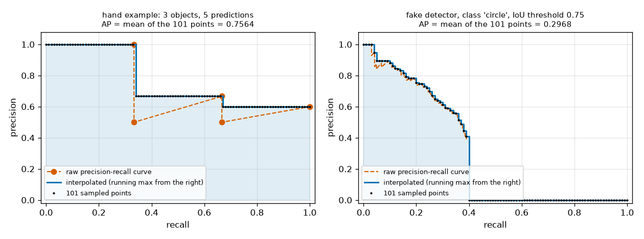
Connecting the five points \((R_k, P_k)\) in order gives the orange dotted line on the left of Figure 3-2. The curve does not descend smoothly; it has a sawtooth shape. The reason can be read straight from the table.
- Accepting one FP leaves recall unchanged and lowers only precision. The curve drops straight down (\(k = 1 \to 2\): recall stays at 0.333, precision 1.000 → 0.500).
- Accepting one TP increases recall by \(1/N_{\mathrm{gt}}\) and raises precision as well. The curve moves up and to the right (\(k = 2 \to 3\): recall 0.333 → 0.667, precision 0.500 → 0.667).
- Figure: Figure 3-2. PR curve — the orange dotted line is the raw curve, the solid blue line is the interpolated curve, and the black dots are the 101 points used to compute AP. The left side is the example in the table above (the sawtooth raw curve and the stepped interpolated curve); the right side is the curve of the fake detector built later in experiment 2 (circle class, IoU threshold 0.75).
Interpolation: shaving off the teeth
Look at a dip in the sawtooth. The point at \(k = 2\) is (recall 0.333, precision 0.500), and the point at \(k = 3\) is (recall 0.667, precision 0.667). The \(k = 3\) point has both higher recall and higher precision. Someone choosing a threshold has no reason to use the threshold corresponding to \(k = 2\), since accepting just one more prediction improves both values.
So when computing AP, these dips are filled in. Each position's precision is replaced with "the highest precision at that position or to its right (positions with equal or higher recall)." This is called the interpolated precision and is written \(\tilde{P}_k\) (P tilde).
\(\tilde{P}_k = \max_{j \ge k} P_j\)
\(\max_{j \ge k}\) means "the largest value from the \(k\)-th position to the end." To compute it, go from the right end to the left, writing down the maximum seen so far (a cumulative maximum).
- Computing interpolated precision — cumulative maximum from the right
- \(\tilde{P}_5 = P_5 = 0.6\). The rightmost position has only itself.
- \(\tilde{P}_4 = \max(P_4, \tilde{P}_5) = \max(0.5,\; 0.6) = 0.6\). The 0.6 to the right is larger than \(P_4 = 0.5\). The dip is filled.
- \(\tilde{P}_3 = \max(P_3, \tilde{P}_4) = \max(0.667,\; 0.6) = 0.667\). \(P_3 = 2/3\) is larger than any value to its right, so it stays as is.
- \(\tilde{P}_2 = \max(P_2, \tilde{P}_3) = \max(0.5,\; 0.667) = 0.667\). The second dip is filled too.
- \(\tilde{P}_1 = \max(P_1, \tilde{P}_2) = \max(1,\; 0.667) = 1 \quad\Longrightarrow\quad \tilde{P} = [1,\; 0.667,\; 0.667,\; 0.6,\; 0.6]\). In the original \(P = [1,\; 0.5,\; 0.667,\; 0.5,\; 0.6]\), the two 0.5 values have been filled. The interpolated values never increase from left to right (they are monotonically decreasing).
Writing interpolated precision as a function of recall \(r\) rather than of rank \(k\) makes the later calculations easier. Write "the highest precision among positions with recall at least \(r\)" as \(p_{\mathrm{interp}}(r)\) (interp stands for interpolated).
\(p_{\mathrm{interp}}(r) = \max_{k \,:\, R_k \ge r} P_k \qquad (0 \text{ if no such } k \text{ exists})\)
In words, it is "the highest precision you can get while achieving a recall of at least \(r\)." In the example above, it forms the following staircase (the blue line on the left of Figure 3-2).
| Range of recall \(r\) | Positions with \(R_k \ge r\) | \(p_{\mathrm{interp}}(r)\) |
| \(0 \le r \le 1/3\) | \(k = 1, 2, 3, 4, 5\) | \(\max(1, 0.5, 0.667, 0.5, 0.6) = 1\) |
| \(1/3 \lt r \le 2/3\) | \(k = 3, 4, 5\) | \(\max(0.667, 0.5, 0.6) = 0.667\) |
| \(2/3 \lt r \le 1\) | \(k = 5\) | \(0.6\) |
Sometimes a detector fails to find all the ground truths, so recall never reaches 1. For example, if the highest recall is 0.4, no position satisfies the condition for \(r \gt 0.4\), so \(p_{\mathrm{interp}}(r) = 0\) there. The right side of Figure 3-2 is such a case: the curve ends around recall 0.4 and is 0 after that. Missed objects are penalized by turning the right side of the PR curve into 0.
AP: the curve as a single number
Area under the curve
The PR curve shows a detector's character well, but comparing two detectors requires a single number. The closer the curve hugs the upper right (the higher the precision even at high recall), the better the detector, so the natural summary is the area under the curve. This is AP (average precision).
\(\mathrm{AP} \approx \int_0^1 p_{\mathrm{interp}}(r)\, dr\)
The integral sign \(\int_0^1 \dots dr\) means "measure the area under the curve as \(r\) moves from 0 to 1." Since the width is 1, the area equals the average precision over the whole recall range, which is where the name "average precision" comes from. A perfect detector has precision 1 at every recall, so its AP = 1, and a detector that finds nothing has AP = 0.
The example above has three steps, so the area can be computed directly. Each step is \(1/3\) wide, with heights 1, 0.667, and 0.6.
\(\frac{1}{3} \times 1 + \frac{1}{3} \times \frac{2}{3} + \frac{1}{3} \times 0.6 = \frac{1 + 0.6667 + 0.6}{3} = 0.7556\)
COCO's 101-point interpolation
Instead of measuring the area exactly, COCO's evaluation program places 101 evenly spaced points on the recall axis and averages the interpolated precision at those points. The points are \(r_i = i/100\), that is, 0, 0.01, 0.02, …, 1.00.
\(\mathrm{AP} = \frac{1}{101} \sum_{i=0}^{100} p_{\mathrm{interp}}\!\left(\frac{i}{100}\right)\)
\(\sum_{i=0}^{100}\) means "add up while varying \(i\) from 0 to 100." In this chapter, AP refers to this formula. Let's compute it step by step for the example above.
- AP for 3 ground truths and predictions TP, FP, TP, FP, TP
- \(r_i \le \tfrac{1}{3} = 0.333\ldots \;\Longleftrightarrow\; i = 0, 1, \dots, 33 \quad (34\text{ points}) \quad\Rightarrow\quad p_{\mathrm{interp}} = 1\). 0.33 is less than \(1/3\) and 0.34 is greater. So the points in the first step are the 34 points from 0.00 to 0.33 (34, not 33, because 0 is included).
- \(\tfrac{1}{3} \lt r_i \le \tfrac{2}{3} = 0.666\ldots \;\Longleftrightarrow\; i = 34, \dots, 66 \quad (33\text{ points}) \quad\Rightarrow\quad p_{\mathrm{interp}} = \tfrac{2}{3}\). 0.66 is less than \(2/3\) and 0.67 is greater. From 0.34 to 0.66 there are \(66 - 34 + 1 = 33\) points.
- \(\tfrac{2}{3} \lt r_i \le 1 \;\Longleftrightarrow\; i = 67, \dots, 100 \quad (34\text{ points}) \quad\Rightarrow\quad p_{\mathrm{interp}} = 0.6\). From 0.67 to 1.00 there are \(100 - 67 + 1 = 34\) points. The point counts of the three intervals add up to \(34 + 33 + 34 = 101\), as they should.
- \(\sum_{i=0}^{100} p_{\mathrm{interp}}(r_i) = 34 \times 1 + 33 \times \tfrac{2}{3} + 34 \times 0.6 = 34 + 22 + 20.4 = 76.4\). For each interval, add (number of points) × (that interval's interpolated precision).
- \(\mathrm{AP} = \frac{76.4}{101} = 0.7564\). Divide by 101. This differs slightly from the exact area of 0.7556 in the third decimal place, because the points do not fall exactly on the interval boundaries.
The code is split into two functions. precision_recall_curve builds the \(P_k\) and \(R_k\) of the table, and average_precision does the interpolation and the 101-point average.
def precision_recall_curve(is_tp: np.ndarray, num_gt: int):
    """점수 내림차순으로 늘어놓은 TP 여부에서 정밀도 · 재현율 곡선을 만든다.

    k 번째 값은 "점수가 높은 순으로 k 개까지만 예측으로 인정했을 때" 의 정밀도 · 재현율이다.
    """
    tp_cum = np.cumsum(is_tp)  # 위에서부터 k 개 가운데 TP 수
    fp_cum = np.cumsum(~is_tp)  # 위에서부터 k 개 가운데 FP 수
    recall = tp_cum / max(num_gt, 1)
    precision = tp_cum / np.maximum(tp_cum + fp_cum, 1)
    return precision, recall


def average_precision(precision: np.ndarray, recall: np.ndarray) -> float:
    """COCO 방식 AP: 재현율 0, 0.01, …, 1.00 의 101개 지점에서 보간한 정밀도의 평균.

    1) 정밀도를 오른쪽부터 누적 최댓값으로 바꿔 톱니를 없앤다 (재현율 r 이상에서 얻을 수 있는 최고 정밀도).
    2) 지점 r 마다, 재현율이 r 이상이 되는 첫 자리의 정밀도를 읽는다. 그런 자리가 없으면 0.
    """
    if len(precision) == 0:
        return 0.0
    envelope = np.maximum.accumulate(precision[::-1])[::-1]
    points = np.linspace(0.0, 1.0, 101)
    index = np.searchsorted(recall, points, side="left")
    sampled = np.where(index < len(envelope), envelope[np.minimum(index, len(envelope) - 1)], 0.0)
    return float(sampled.mean())
-
np.cumsum(is_tp)is a cumulative sum. Given[True, False, True, False, True], it returns[1, 1, 2, 2, 3], which is the "Cumulative TP" column of the table.~is_tpflips true and false, so its cumulative sum is the "Cumulative FP" column. -
np.maximum.accumulate(precision[::-1])[::-1]is the "cumulative maximum from the right." It reverses the array ([::-1]), takes the cumulative maximum from the left, and reverses the result again. -
np.searchsorted(recall, points, side="left")finds, for each point \(r\), "the first position where recall reaches at least \(r\)." Recall is a non-decreasing array, so a binary search works. The interpolated precision at that position is exactly \(p_{\mathrm{interp}}(r)\). - If there is no such position (
indexequals the array length), 0 is used. That is the part of the recall range the detector never reached.
  정밀도   [1.0, 0.5, 0.667, 0.5, 0.6]
  재현율   [0.333, 0.333, 0.667, 0.667, 1.0]
  보간 정밀도 [1.0, 0.667, 0.667, 0.6, 0.6]
  AP (101점) 0.7564 | 손계산 (34·1 + 33·(2/3) + 34·0.6)/101 = 0.7564
  참고: 11점 방식 0.7636, 보간 곡선 아래의 정확한 넓이 0.7556
The hand calculation and the code give the same value, 0.7564. On top of this, the practice file checks average_precision on 300 random inputs against a slow implementation that follows the definition literally: "for each point, take the maximum precision among positions with recall at least \(r\), then average."
A difference of \(2.2 \times 10^{-15}\) is at the level of the error that arises because computers represent real numbers with a finite number of digits, so the two calculations can be considered identical. (The NMS on the second line is covered later in this chapter.)
Note: the 11-point method. How many points to use is a matter of convention. PASCAL VOC, the leading benchmark before COCO, at one time used only 11 points, at recall 0, 0.1, …, 1.0. Computing the example above with 11 points gives 1 at the 4 points from 0 to 0.3, 0.667 at the 3 points from 0.4 to 0.6, and 0.6 at the 4 points from 0.7 to 1.0, so the result is \((4 + 2 + 2.4)/11 = 0.7636\). The same detections give slightly different values, 0.7636, 0.7564, and 0.7556, depending on the method. So compare AP values only when they were computed the same way. When papers today report COCO AP, they all use the 101-point method of COCO's official evaluation program (pycocotools).
Four properties of AP
Here are some properties that follow directly from the definition. The experiments later confirm each of them visually.
- No score threshold needs to be chosen. AP looks at precision and recall at all thresholds at once. So the ranking of detectors never flips depending on "where the threshold was set."
- Only the order of the scores matters, not their magnitude. Halving all the scores, or squaring them, leaves AP unchanged as long as the order stays the same. Conversely, AP changes when the order of the scores changes, even if not a single box changes.
- Early FPs are expensive; FPs at the very end are free. A high-scoring FP lowers the precision at every position after it. On the other hand, an FP that scores lower than the last TP cannot change AP at all. Its own position has low precision, but interpolation takes "the maximum to the right," so it cannot affect positions to its left, and all 101 points read their values from earlier positions.
- Missed objects remain as zeros that cannot be filled. If the highest recall is \(R_{\max}\), all points to its right are 0, so AP roughly cannot exceed \(R_{\max}\).
Let's check the third property with the earlier example. Appending 100 FPs with score 0.1 after the five predictions leaves unchanged the positions that first satisfy \(R_k \ge r\) (positions 1, 3, and 5) and their interpolated precision. The appended positions have precision \(3/6, 3/7, \dots\), all less than \(P_5 = 0.6\), so they cannot change the cumulative maximum. AP is still 0.7564.
mAP and the COCO metrics
Averaging over classes
So far, AP has been a value for one class. In the shapes world, there is a separate "circle AP," "rectangle AP," and "triangle AP." The score for the detector as a whole is their average over classes, called mAP (mean average precision). With \(C\) classes and \(\mathrm{AP}_c\) the AP of class \(c\),
\(\mathrm{mAP} = \frac{1}{C} \sum_{c=1}^{C} \mathrm{AP}_c\)
Because each class is computed separately and then averaged, classes with many objects and classes with few carry the same weight. In COCO, there are nearly 270,000 people in the training and validation sets of the 2014 release alone (according to the COCO paper), yet the AP for people and the AP for much rarer classes each enter mAP with the same weight of \(1/C\). This keeps a detector that does well only on common classes from scoring high.
Averaging over ten IoU thresholds
Earlier, raising the IoU threshold \(\tau\) from 0.5 to 0.75 reduced the TPs for the same predictions from 2 to 1. With \(\tau = 0.5\) alone, "a box barely hanging on at IoU 0.51" and "a box fitting snugly at IoU 0.95" are equally TPs. How accurately the boxes are drawn does not show up in the score.
COCO solves this by computing AP at each of 10 thresholds and averaging the results. The thresholds run from 0.50 to 0.95 in steps of 0.05. Writing \(\mathrm{AP}_c^{\tau}\) for the AP of class \(c\) scored with IoU threshold \(\tau\), COCO's headline metric is:
\(\mathrm{AP} = \frac{1}{10} \sum_{\tau \in \{0.50,\, 0.55,\, \dots,\, 0.95\}} \;\frac{1}{C} \sum_{c=1}^{C} \mathrm{AP}_c^{\tau}\)
This metric is written in many ways: AP@[.50:.05:.95], AP@[.5:.95], AP50:95, mAP@50:95. They all mean the same thing (the RF-DETR paper itself uses AP in its tables and mAP 50:95 in the text). The official COCO documentation explains that averaging over multiple thresholds "rewards detectors with better localization."
Caution: in COCO, AP and mAP mean the same thing. In the original sense, AP is the value for one class and mAP is their average. However, the official COCO documentation states that AP is averaged over all categories, that this is traditionally called mAP, and that "we make no distinction between AP and mAP." So the "AP" in today's paper tables is already averaged over classes and over IoU thresholds. From here on, this tutorial also uses plain "AP" to mean the value of the formula above (averaged over classes and over the 10 thresholds). For a single class at a single threshold, it adds subscripts as in \(\mathrm{AP}_c^{\tau}\) or says so explicitly.
COCO uses 80 classes, so a single AP number averages the readings at 101 points on each of 10 × 80 = 800 PR curves. A great deal is compressed into one number, which is why papers also report several breakdowns of it.
COCO's six metrics
Of the detection metrics defined in the official COCO documentation, the following six appear in nearly every paper's tables.
| Metric | Definition | What it measures |
| AP | Average over IoU thresholds 0.50, 0.55, …, 0.95 | The headline metric. Finding objects and drawing accurate boxes, together |
| AP50 | IoU threshold 0.50 only | "Did it find the object, even roughly?" The old PASCAL VOC criterion |
| AP75 | IoU threshold 0.75 only | "Is the box fairly accurate?" The official documentation calls it the strict metric |
| APS | Only objects with area smaller than 32² pixels | Small objects |
| APM | Only objects with area between 32² and 96² pixels | Medium objects |
| APL | Only objects with area larger than 96² pixels | Large objects |
- AP50 (AP at IoU = 0.50) and AP75 (AP at IoU = 0.75) keep only a single \(\tau\) in the formula above. A high AP50 with a low AP75 means "it finds objects, but the boxes are loose." The smaller the gap between the two, the more accurate the boxes.
- AP by size (APS, APM, APL) splits the ground-truth objects into three groups by area and computes AP (averaged over the 10 thresholds) separately for each group. The boundaries are \(32^2 = 1024\) pixels and \(96^2 = 9216\) pixels. Area is measured in pixels of the original image, and COCO uses the number of pixels covered by the object's segmentation mask, not by its box. According to the official documentation, about 41% of COCO objects are small, 34% medium, and 24% large. Small objects are the most numerous and, as shown later, the hardest.
- Every metric is computed accepting at most the top 100 predictions by score per image. This rule prevents forcing recall up by spewing out thousands of boxes. Even if a DETR-family detector with 300 queries outputs 300 predictions, only the top 100 per image by score are used for scoring.
Note: the COCO dataset. COCO (Common Objects in Context) is a dataset created by Lin et al. (2014). The paper introduces it as a dataset of 91 object types, 328,000 images, and 2.5 million labeled instances, and states that the 2014 release was limited to 80 classes among them. These 80 classes are what detection benchmarks use. Regions where objects are hard to separate individually, such as dense crowds of people, are marked separately as "crowd," and these regions are ignored during scoring (predictions inside them are neither TPs nor FPs). A broader introduction to the dataset is in chapter 1.
Seeing the two averages in numbers
Let's look concretely at which numbers the "threshold average" and the "class average" are averages of. Below is the output of scoring one fake detector from experiment 1 later on (noise 0.10) on the shapes-world validation set.
  sigma 0.10 의 IoU 문턱값별 AP(클래스 평균): 0.971 0.898 0.771 0.558 0.345 0.170 0.047 0.008 0.001 0.000
    → 열 개의 평균 0.377
    IoU 0.50 에서의 클래스별 AP: circle 0.981, rectangle 0.970, triangle 0.960 → 평균 0.971
- How a single AP number is produced
- \(\mathrm{AP}_{50} = \frac{0.981 + 0.970 + 0.960}{3} = \frac{2.911}{3} = 0.970\). Average the APs of the three classes (circle, rectangle, triangle) at IoU threshold 0.50. It differs from the 0.971 in the output in the last digit because the three values were already rounded to three decimal places.
- \(\sum_{\tau} = 0.971 + 0.898 + 0.771 + 0.558 + 0.345 + 0.170 + 0.047 + 0.008 + 0.001 + 0.000 = 3.769\). Add up the ten class averages obtained the same way at each threshold 0.50, 0.55, …, 0.95. The first value is AP50, and the sixth value, 0.170, is AP75.
- \(\mathrm{AP} = \frac{3.769}{10} = 0.377\). Divide by 10. This detector has an almost perfect AP50 of 0.971, but the values collapse quickly as the threshold gets stricter, so its AP is only 0.377.
Papers multiply this value by 100 and write it as 37.7. "48.0 AP" means 0.480.
Walking through the scoring code
evaluate_ap stitches together all the pieces covered so far. From chapter 7 on, every detector in this tutorial is scored with this function.
def evaluate_ap(predictions, targets, num_classes: int, iou_thresholds=COCO_IOU_THRESHOLDS, max_dets: int = 100):
    """데이터셋 전체를 채점한다.

    predictions[i]: {"boxes": (n, 4) 정규화 (cx, cy, w, h), "scores": (n,), "labels": (n,)} — i 번째 그림의 예측
    targets[i]:     {"boxes": (m, 4) 정규화 (cx, cy, w, h), "labels": (m,)}                — i 번째 그림의 정답

    돌려주는 값: {"AP": IoU 문턱값 전체 평균, "AP50": …, "AP75": …,
                 "per_class": 클래스별 AP (문턱값 평균), "table": (문턱값 수, 클래스 수) 배열}
    정답이 하나도 없는 클래스는 평균에서 뺀다 (COCO 와 같다).
    """
    table = np.full((len(iou_thresholds), num_classes), np.nan)
    for cls in range(num_classes):
        num_gt = sum(int((t["labels"] == cls).sum()) for t in targets)
        if num_gt == 0:
            continue
        for ti, threshold in enumerate(iou_thresholds):
            scores_all, tp_all = [], []
            for pred, target in zip(predictions, targets):
                scores = pred["scores"].detach().cpu()
                keep = torch.argsort(scores, descending=True, stable=True)[:max_dets]  # 그림마다 점수 상위 max_dets 개만
                labels = pred["labels"].detach().cpu()[keep]
                boxes = box_cxcywh_to_xyxy(pred["boxes"].detach().cpu()[keep])
                scores = scores[keep]
                chosen = labels == cls
                gt_boxes = box_cxcywh_to_xyxy(target["boxes"].cpu()[target["labels"].cpu() == cls])
                is_tp = match_detections(boxes[chosen], scores[chosen], gt_boxes, threshold)
                scores_all.append(torch.sort(scores[chosen], descending=True).values)
                tp_all.append(is_tp)
            scores_all = torch.cat(scores_all).numpy()
            tp_all = torch.cat(tp_all).numpy()
            order = np.argsort(-scores_all, kind="stable")  # 모든 그림의 예측을 점수 순으로 한 줄로
            precision, recall = precision_recall_curve(tp_all[order], num_gt)
            table[ti, cls] = average_precision(precision, recall)
    per_threshold = np.nanmean(table, axis=1)
    result = {
        "AP": float(np.nanmean(per_threshold)),
        "per_class": np.nanmean(table, axis=0),
        "table": table,
    }
    for name, value in (("AP50", 0.5), ("AP75", 0.75)):
        if value in iou_thresholds:
            result[name] = float(per_threshold[iou_thresholds.index(value)])
    return result
The inputs are per-image lists of predictions and ground truths. Boxes are \((c_x, c_y, w, h)\) normalized to 0–1 (chapter 2), and they are converted to \((x_0, y_0, x_1, y_1)\) inside the function. Reading the three nested loops from the outside in brings up this chapter's content in order.
- For each class (
for cls): count the number of ground truths \(N_{\mathrm{gt}}\) for that class across the whole dataset. A class with no ground truths at all has a zero denominator for recall, so its AP is undefined and it is skipped (it stays asnanin the table and drops out of the averages). - For each IoU threshold (
for ti, threshold): the default isCOCO_IOU_THRESHOLDS, the ten values 0.50, 0.55, …, 0.95. - For each image (
for pred, target): first keep only the topmax_dets(100) predictions in that image by score. Among them, pick the predictions of the current class and the ground truths of the current class, and match them withmatch_detections. Collect the results (TP or not) and the scores in lists. Matching happens only within an image. A prediction in image 3 can never be matched to a ground truth in image 7. - Line up in one row: concatenate the scores and TP flags collected from all images (
torch.cat) and sort by score in descending order (np.argsort(-scores_all)). Ranking is done across the whole dataset. - PR curve and AP: call
precision_recall_curveand thenaverage_precisionto get a single value, and record it in the tabletable[threshold, class]. The table's shape is(10, number of classes). - Averaging: averaging the table across classes gives the ten per-threshold APs (
per_threshold), and averaging those again gives"AP". The values at thresholds 0.5 and 0.75 are also returned separately as"AP50"and"AP75".
The contrast between steps 3 and 4 is important. Whether a prediction is right or wrong is decided within an image, but ranking ignores image boundaries. So a detector's scores must be comparable across images. AP comes out high only if a 0.9 on an easy image means the same degree of "trustworthiness" as a 0.9 on a hard image.
- Note — differences from the official evaluation program (pycocotools)
-
evaluate_apfollows the core computations of COCO's official evaluation program, pycocotools (greedy matching, 101-point interpolation, averaging over 10 thresholds), exactly, but leaves out parts the shapes world does not need.
- There are no crowd regions. pycocotools counts predictions that overlap ground truths marked as crowd as neither TP nor FP. The shapes world has no such ground truths.
- Size-based metrics (APS, APM, APL) and average recall (AR) are not computed. Shapes-world images are 96×96 and the shapes are 13–40 pixels on a side, so splitting them by COCO's 32² and 96² boundaries is meaningless.
- "At most 100 per image" is counted differently. Following the description in the official documentation, this function keeps the top 100 across all classes in an image combined. The pycocotools code keeps the top 100 per image per class. If an image has no more than 100 predictions, the two approaches give the same result.
- The order of predictions with exactly equal scores can differ depending on the sorting method.
While writing this chapter, the original author also scored four sets of fake detections with pycocotools 2.0.11 for comparison (this is not included in the practice file; pycocotools is not a required package for this tutorial). In the two cases with no tied scores and at most 100 predictions per image, AP, AP50, and AP75 matched to 15 decimal places. The case with tied scores differed in AP by \(6 \times 10^{-5}\), and the case with more than 100 predictions per image by \(1.2 \times 10^{-4}\); making the scores distinct or removing the 100 limit, respectively, brought them back into agreement to 15 places. In other words, the differences came only from the third and fourth items above. Even so, COCO scores for publication in a paper must be computed with the official program.
Experiments: what AP responds to
Knowing the definition and having a feel for it are two different things. In this section, we poke at AP directly. Since no detector has been built yet (that starts in chapter 7), we use "fake detectors" made by deliberately corrupting the ground truth. The nice thing about a fake detector is that we know exactly what is wrong and by how much. By jittering only the boxes, changing only the scores, or adding only duplicates, we can see separately how AP responds to each.
Building a fake detector
The stage is the shapes-world validation set (ShapesDataset(500, seed=1)). It has 1,265 objects across 500 images (428 circles, 445 rectangles, 392 triangles). Scoring needs only the ground-truth boxes and classes, not the images themselves. The fake detector has three adjustable settings.
- Box position noise
sigma: for each ground-truth box, it makes one prediction, shifting the center by a Gaussian random amount with standard deviation "box size × sigma" and multiplying the width and height by \(e^{\text{sigma} \times z}\) (\(z\) is a standard normal random number). With sigma 0 the prediction is exactly the ground truth; with 0.1 the box is off by about 10% of its size and grows or shrinks by about 10%. The class always stays the same as the ground truth. - Scoring method
score_mode: use the IoU between the box and the ground truth directly as the score ("iou"), add noise to it ("noisy_iou"), use a random number unrelated to the box ("random"), or use the reverse, \(1 - \operatorname{IoU}\) ("inverse"). - Extra predictions:
duplicates, which predict the same object again (duplicate predictions), andjunk, boxes placed anywhere (junk predictions).
def jitter_boxes(boxes: torch.Tensor, sigma: float, rng: np.random.Generator) -> torch.Tensor:
    """박스 (n, 4) (cx, cy, w, h) 에 위치 잡음을 넣는다.

    중심은 박스 크기의 sigma 배를 표준편차로 하는 가우시안만큼 옮기고 (큰 박스는 많이, 작은 박스는 조금),
    너비 · 높이에는 exp(sigma · 표준 정규) 를 곱한다 (sigma = 0.1 이면 대략 ±10% 늘거나 준다).
    """
    noise = torch.from_numpy(rng.normal(size=tuple(boxes.shape)).astype(np.float32))
    cx, cy, w, h = boxes.unbind(-1)
    return torch.stack([cx + sigma * w * noise[:, 0], cy + sigma * h * noise[:, 1],
                        w * torch.exp(sigma * noise[:, 2]), h * torch.exp(sigma * noise[:, 3])], dim=-1)


def make_scores(iou: torch.Tensor, mode: str, rng: np.random.Generator) -> torch.Tensor:
    """예측마다 점수를 붙인다. iou 는 그 예측과 (그것을 만든) 정답 박스의 IoU.

    "iou"       점수 = IoU. 박스가 정확할수록 점수가 높다 (이상적인 점수).
    "noisy_iou" 점수 = IoU + 표준편차 0.1 의 잡음. 대체로 맞지만 가끔 순서가 뒤집힌다.
    "random"    점수 = 0.5 – 1 의 균등 난수. 박스의 질과 아무 상관이 없다.
    "inverse"   점수 = 1 − IoU. 박스가 나쁠수록 점수가 높다 (최악의 점수).
    """
    n = len(iou)
    if mode == "iou":
        return iou.clone()
    if mode == "noisy_iou":
        # 위쪽은 자르지 않는다: 1 에서 자르면 점수가 같은 예측이 여럿 생겨 순서가 모호해진다.
        # 점수가 1 을 조금 넘어도 AP 는 점수의 크기가 아니라 순서만 본다.
        return (iou + 0.1 * torch.from_numpy(rng.normal(size=n).astype(np.float32))).clamp(min=0.01)
    if mode == "random":
        return torch.from_numpy(rng.uniform(0.5, 1.0, size=n).astype(np.float32))
    if mode == "inverse":
        return 1.0 - iou
    raise ValueError(mode)


def fake_detector(targets, seed: int, sigma: float = 0.0, score_mode: str = "random", duplicates: int = 0,
                  duplicate_score_scale: float = 1.0, junk: int = 0, junk_score=(0.01, 0.2)):
    """정답을 흔들어 만든 가짜 탐지 결과. evaluate_ap 가 받는 predictions 형식으로 돌려준다.

    - 정답 박스마다 예측 하나: 위치 잡음 sigma 를 넣고, 클래스는 정답 그대로, 점수는 score_mode 로.
    - duplicates: 정답마다 같은 방법으로 따로 흔든 박스를 그만큼 더 낸다 (같은 객체를 여러 번 예측).
      그 점수에는 duplicate_score_scale 을 곱한다 (1 이면 원래 예측과 비슷한 점수, 0.3 이면 낮은 점수).
    - junk: 그림마다 아무 데나 놓은 박스(헛예측)를 그만큼 더 낸다. 클래스는 무작위, 점수는 junk_score 구간의 균등 난수.

    난수를 셋으로 나눠 쓴다: 박스용 · 점수용 · 추가분(중복 · 헛예측)용. 그래서 sigma 와 score_mode 가 같으면
    duplicates · junk 를 바꿔도 "원래 예측" 은 박스도 점수도 똑같다. score_mode 만 바꾸면 박스는 똑같다.
    """
    box_rng = np.random.default_rng([seed, 0])
    score_rng = np.random.default_rng([seed, 1])
    extra_rng = np.random.default_rng([seed, 2])
    predictions = []
    for target in targets:
        gt_boxes, gt_labels = target["boxes"], target["labels"]
        gt_xyxy = box_cxcywh_to_xyxy(gt_boxes)
        boxes = jitter_boxes(gt_boxes, sigma, box_rng)
        iou = paired_box_iou(box_cxcywh_to_xyxy(boxes), gt_xyxy)  # 예측 k 와 정답 k 의 IoU, (객체 수,)
        all_boxes, all_scores, all_labels = [boxes], [make_scores(iou, score_mode, score_rng)], [gt_labels]
        for _ in range(duplicates):
            copy = jitter_boxes(gt_boxes, sigma, extra_rng)
            copy_iou = paired_box_iou(box_cxcywh_to_xyxy(copy), gt_xyxy)
            all_boxes.append(copy)
            all_scores.append(make_scores(copy_iou, score_mode, extra_rng) * duplicate_score_scale)
            all_labels.append(gt_labels)
        if junk > 0:
            wh = extra_rng.uniform(0.14, 0.42, size=(junk, 2))
            center = extra_rng.uniform(wh / 2, 1 - wh / 2)  # 그림 밖으로 나가지 않게
            all_boxes.append(torch.from_numpy(np.concatenate([center, wh], axis=1).astype(np.float32)))
            all_scores.append(torch.from_numpy(extra_rng.uniform(*junk_score, size=junk).astype(np.float32)))
            all_labels.append(torch.from_numpy(extra_rng.integers(0, NUM_CLASSES, size=junk)))
        predictions.append({"boxes": torch.cat(all_boxes), "scores": torch.cat(all_scores), "labels": torch.cat(all_labels)})
    return predictions
The one thing worth pointing out in the code is that it uses three random number generators: one for boxes, one for scores, and one for extras. Thanks to this, changing only score_mode changes only the scores, leaving the boxes exactly the same, and changing duplicates or junk changes only what is added while leaving the original predictions as they are. Changing one thing at a time in the experiments requires this kind of setup.
- Figure: Figure 3-3. Visualizing the size of the noise sigma — two shapes-world images overlaid with ground-truth boxes (solid green) and fake predicted boxes with noise 0, 0.04, 0.10, and 0.20 (dashed magenta). The numbers above the images are the IoU between each prediction and its ground truth.
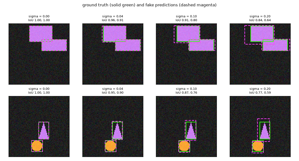
Get a rough sense of scale from Figure 3-3. With sigma = 0.04 the boxes look almost exactly overlaid on the ground truth (IoU 0.9 or above), sigma = 0.10 looks "a little loose" (IoU 0.76–0.91), and sigma = 0.20 is visibly off (IoU 0.59–0.84). To the human eye, even 0.10 looks like a good detection. How does AP see it?
Experiment 1: when the boxes jitter
Score while increasing the noise from 0 to 0.30. The scores are random numbers unrelated to the boxes ("random"), so the only thing that changes is the boxes.
검증 세트: 그림 500장, 객체 1265개 (circle 428, rectangle 445, triangle 392)
[3] 실험 1 · 박스 위치 잡음 (점수는 무작위)
  sigma | 평균 IoU | AP50  | AP75  | AP
   0.00 |    1.000 | 1.000 | 1.000 | 1.000
   0.02 |    0.932 | 1.000 | 1.000 | 0.885
   0.04 |    0.871 | 1.000 | 0.976 | 0.738
   0.06 |    0.814 | 1.000 | 0.676 | 0.604
   0.08 |    0.763 | 0.997 | 0.349 | 0.485
   0.10 |    0.715 | 0.971 | 0.170 | 0.377
   0.15 |    0.611 | 0.652 | 0.022 | 0.171
   0.20 |    0.523 | 0.327 | 0.003 | 0.069
   0.30 |    0.386 | 0.068 | 0.000 | 0.012
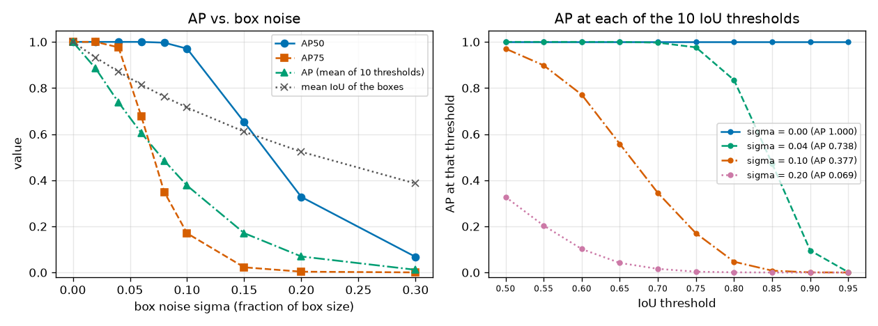
- Figure: Figure 3-4. Box noise and AP — the left side shows AP50 (blue), AP75 (orange), AP (green), and the mean IoU of the boxes (gray dotted) as the box noise increases. The right side shows the AP at each of the 10 IoU thresholds for four noise levels. The AP in the legend is the average of those ten points.
Here is what to read from the table and Figure 3-4.
- Perfect predictions give AP = 1 (sigma = 0). This also confirms that the code gets the basics right.
- AP75 collapses first. As sigma goes from 0.04 to 0.10, AP50 stays almost the same (1.000 → 0.971), while AP75 plunges from 0.976 to 0.170. As the mean IoU dropped from 0.87 to 0.72, most predictions fell below the 0.75 threshold. AP50 collapses only after sigma passes 0.10 and the mean IoU falls to around 0.6 (0.652 at sigma = 0.15).
- AP reacts earliest of all. At sigma = 0.02, AP50 and AP75 are still perfect, but AP is 0.885. AP includes very strict thresholds such as 0.90 and 0.95, and many boxes fail to clear them even with a mean IoU of 0.93. The green line (sigma = 0.04) on the right of Figure 3-4 shows this: it stays near 1 up to 0.75, then falls steeply and reaches 0 at 0.95.
- AP is not the mean IoU. At sigma = 0.10, the mean IoU is 0.715 but AP is 0.377. AP comes not from the average IoU but from "the fraction of predictions that clear the threshold," so it changes in steps around each threshold. The sigma = 0.10 boxes, which looked only "a little loose" in Figure 3-3, score 37.7 under COCO's scoring.
The right-hand plot suggests a good way to read the AP number: AP is the average height of the ten points on this curve. As the boxes become more accurate, the whole curve shifts to the right and AP rises. AP50 is just the single point at the left end of the curve, and AP75 a single point in the middle.
Experiment 2: same boxes, different scores
This time the boxes are fixed. The 1,265 boxes made with sigma = 0.10 are kept as they are, and only the scores are assigned, in four different ways.
[4] 실험 2 · 점수의 질 (박스는 모두 같다: sigma = 0.1)
  예측 1265개 가운데 정답과 IoU ≥ 0.50 인 비율 0.984, IoU ≥ 0.75 인 비율 0.391
  iou       | AP50 0.980 | AP75 0.393 | AP 0.480
  noisy_iou | AP50 0.979 | AP75 0.301 | AP 0.443
  random    | AP50 0.971 | AP75 0.170 | AP 0.377
  inverse   | AP50 0.964 | AP75 0.153 | AP 0.369
  참고: 비율의 제곱 0.969 (IoU 0.50), 0.153 (IoU 0.75)
- Figure: Figure 3-5. Four detection results with identical boxes and different scores — the left side shows the PR curves of the four methods for the circle class scored at IoU threshold 0.75; the right side shows bars of AP50, AP75, and AP for the four methods.
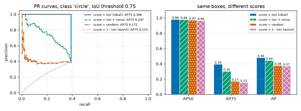
Not a single box differs, yet AP ranges from 0.369 to 0.480. Looking at AP75 alone, it is 0.153 versus 0.393, a difference of more than 2.5 times. The PR curves on the left of Figure 3-5 show why.
- Score = IoU (solid blue): the predictions with IoU of at least 0.75, that is, the TPs, all come first. Precision stays at 1 throughout and the curve ends at recall 0.39, where the TPs run out.
- Score = random (orange dash-dot): TPs and FPs are mixed together, so precision is around 0.39 wherever you cut.
- Score = 1 − IoU (pink dotted): the FPs all come first. Precision starts at 0 and reaches 0.39 only at the end.
- Score = IoU + noise (green dashed): somewhere in between. Good boxes generally come first, but the order sometimes flips.
The AP in these cases can be predicted with a simple calculation. Suppose the number of predictions equals the number of ground truths and the fraction of TPs among the predictions is \(q\) (here, at IoU threshold 0.75, \(q = 0.391\)).
- Why the AP of the same boxes ranges from q to q² depending on score order
- \(R_{\max} = \frac{\text{number of TPs}}{N_{\mathrm{gt}}} = q\). However the scores are assigned, the number of TPs is the same, so the recall when everything is accepted is \(q\) in every case. The interpolated precision at points with \(r \gt q\) is 0.
- \(\text{best order (TPs first):}\quad p_{\mathrm{interp}}(r) = 1 \;\;(r \le q) \quad\Rightarrow\quad \mathrm{AP} \approx 1 \times q = q\). While only TPs are being accepted, precision is 1. This is the area of a rectangle of height 1 and width \(q\).
- \(\text{worst order (FPs first):}\quad p_{\mathrm{interp}}(r) = q \;\;(r \le q) \quad\Rightarrow\quad \mathrm{AP} \approx q \times q = q^2\). The TPs appear only after all the FPs have been accepted, so precision keeps rising and reaches \(\mathrm{TP}/\text{number of predictions} = q\) at the last position. Interpolation takes the maximum to the right, so every position is filled with \(q\). This is a rectangle of height \(q\) and width \(q\).
- \(q = 0.391:\qquad q = 0.391 \;(\text{experiment: } 0.393), \qquad q^2 = 0.153 \;(\text{experiment: } 0.153)\). These match the AP75 values from the experiment. With a random order, precision fluctuates around \(q\) everywhere, giving 0.170, slightly higher than \(q^2\). That is the benefit of interpolation picking out the peaks of the sawtooth.
At AP50, the four methods are nearly the same (0.964–0.980). 98.4% of the predictions are already TPs, so however they are ordered, there are almost no FPs to mix in. Score order matters when TPs and FPs are mixed. And at strict thresholds, they always are.
- Key point — what makes a good score
- Drawing boxes well is not enough to raise AP. The more accurate a prediction's box, the higher its score must be. A detector's score usually comes from its classification confidence that "there is a circle in this box," but confidence in the classification does not guarantee that the box is accurate. To reduce this mismatch, methods were developed that mix the IoU between the predicted box and the ground truth into the training target for the classification score; the IoU-aware BCE loss (IA-BCE) used by LW-DETR and RF-DETR is one of them. It is covered in chapter 9.
Experiment 3: duplicate and junk predictions
Finally, let's add predictions. The baseline is a fairly good detector with sigma = 0.05 and score = IoU + noise. Two kinds of predictions are added to it.
- Duplicate predictions: for each object, 1 or 3 extra boxes jittered separately in the same way. Their scores are assigned the same way as the original predictions ("similar scores") or additionally multiplied by 0.3 ("low scores").
- Junk predictions: 20 or 96 extra boxes per image, placed anywhere. The class is random, and the score is a random number in 0.01–0.2 ("low scores") or 0.5–1.0 ("high scores").
[5] 실험 3 · 중복 예측, 헛예측, NMS (sigma = 0.05, 점수 = IoU + 잡음)
  기본 (객체마다 예측 1개)              | 그림당 예측   2.53개 | AP50 1.000 | AP75 0.911 | AP 0.700
  + 중복 1개씩, 낮은 점수(×0.3)        | 그림당 예측   5.06개 | AP50 1.000 | AP75 0.951 | AP 0.730
  + 중복 1개씩, 비슷한 점수             | 그림당 예측   5.06개 | AP50 0.846 | AP75 0.832 | AP 0.644
  + 중복 3개씩, 비슷한 점수             | 그림당 예측  10.12개 | AP50 0.763 | AP75 0.759 | AP 0.608
  + 헛예측 20개씩, 낮은 점수            | 그림당 예측  22.53개 | AP50 1.000 | AP75 0.911 | AP 0.700
  + 헛예측 96개씩, 낮은 점수            | 그림당 예측  98.53개 | AP50 1.000 | AP75 0.911 | AP 0.700
  + 헛예측 20개씩, 높은 점수            | 그림당 예측  22.53개 | AP50 0.266 | AP75 0.244 | AP 0.192
- Figure: Figure 3-6. Effect of duplicate predictions, junk predictions, and NMS on AP — horizontal bars comparing AP50, AP75, and AP for eight cases: the baseline, duplicate predictions, NMS after duplicates, and junk predictions. The fifth row from the top (NMS after 3 duplicates) is explained in the next section.
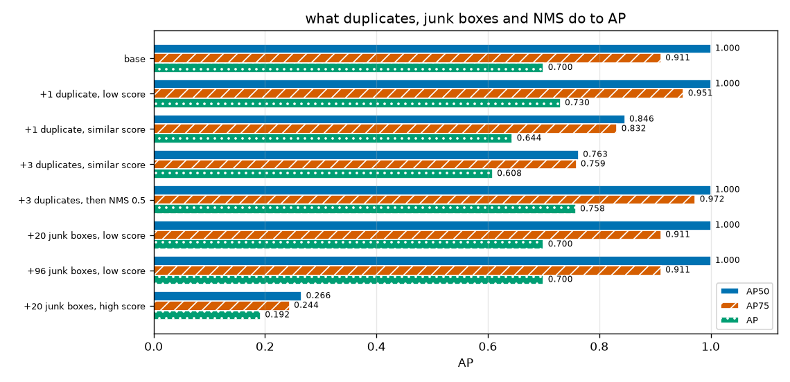
Let's go through the results one at a time.
- Duplicate predictions with similar scores cut AP significantly. Adding just one per object drops AP50 from 1.000 to 0.846, and adding three per object drops it to 0.763, even though the boxes themselves are all fine. The scoring rule gives only one TP per object, so the rest become FPs, and since their scores are similar, those FPs slip in all over the front of the ranking and erode precision.
- Duplicate predictions with low scores do no harm, and here they even helped (AP 0.700 → 0.730). With low scores they sit at the back of the ranking and cannot affect the precision at the front. There is also a bonus: if an original prediction failed to clear a strict threshold and its object is still unmatched, a trailing duplicate that clears the threshold gets a second chance and becomes a TP. That is why AP75 rose from 0.911 to 0.951. This holds, however, only when the "low scores" are clearly lower than those of the original predictions.
- Junk predictions with low scores cannot change AP, no matter how many there are. Adding 20 per image, or even 96 to bring the total close to 100 predictions per image, leaves all three metrics unchanged to three decimal places. This is exactly the third property of AP seen earlier: "FPs at the very end are free." The scores of the junk predictions (0.2 or less) were lower than those of the real predictions, so they all ended up at the very back of the ranking.
- Junk predictions with high scores are devastating. The same 20, with their scores raised to 0.5–1.0, dropped AP from 0.700 to 0.192. Unsurprisingly, since 20 FPs slipped in among about 2.5 real predictions.
- Key point — why DETR can output all 300 queries
- The DETR-family detectors in chapter 7 output a fixed number of predictions (300 queries for RF-DETR) no matter how many objects an image contains. For an image with 3 objects, 297 of them are junk predictions. The third result above is exactly why that is fine: as long as the leftover predictions carry low scores, AP is not reduced at all. Put the other way around, what the detector has to learn is to give "low scores to queries with no object, and a high score to only one of several queries pointing at the same object." The first result above shows how costly duplicate predictions with similar scores are.
The fact that AP does not penalize low-scoring junk predictions is also one of its blind spots. In actual use, you have to set a single score threshold and discard everything below it, and then you need to look again at "single-threshold" metrics such as precision, recall, and F1. Two detectors with the same AP can perform differently at a threshold suitable for practical use.
NMS: removing overlapping predictions
Why it is needed
Experiment 3 showed that duplicate predictions with similar scores cut AP significantly. This is not a concern only for fake detectors. Most detectors before DETR actually produce this kind of output.
The grid- and anchor-based detectors seen in chapter 1 (the YOLO family and others) divide the image into a dense grid and make one prediction per cell (or per anchor, if a cell has several anchors, which are predefined reference boxes). One object usually spans several cells, so several neighboring cells each output a box pointing at the same object. Those cells do not know what the others predicted. The DETR paper (Carion et al., 2020) wrote that the performance of such detectors is "significantly influenced by postprocessing steps to collapse near-duplicate predictions." The standard for that post-processing is NMS (non-maximum suppression). The name means "suppressing whatever is not the maximum": among overlapping boxes, it keeps only the one with the highest score and removes the rest.
Algorithm
The input is the predicted boxes and scores for one class, plus a threshold (the NMS threshold).
- Line up the boxes in descending order of score. This is the "candidate list."
- Take the top box out of the candidate list and put it in the keep list.
- From the boxes remaining in the candidate list, remove every box whose IoU with the box just taken exceeds the threshold (it is treated as a duplicate pointing at the same object).
- Repeat steps 2–3 until the candidate list is empty.
This resembles the scoring rules above, but with a crucial difference. Scoring sorted out duplicates by looking at the ground truth, but NMS does not know the ground truth (there is none at inference time). So it sorts out duplicates using a guess: "boxes that overlap a lot are probably the same object." The cases where this guess is wrong are NMS's weakness.
NMS by hand
There are five boxes, A–E, of the same class. As before, coordinates are \((x_0, y_0, x_1, y_1)\) in grid units. (C in this section is the name of a box, unrelated to the \(C\) used earlier for the number of classes.)
| Box | \((x_0, y_0, x_1, y_1)\) | Area | Score |
| A | (1, 1, 5, 5) | 16 | 0.9 |
| B | (2, 1, 6, 5) | 16 | 0.8 |
| C | (1, 2, 5, 6) | 16 | 0.7 |
| D | (6, 6, 9, 9) | 9 | 0.6 |
| E | (6, 6, 9, 10) | 12 | 0.5 |
Figure 3-7 in the original shows the five boxes before NMS on the left, the boxes A and D that remain after NMS (threshold 0.5) in the middle, and the removed boxes with their IoUs on the right. If the three boxes at the upper left (A, B, C) and the two at the lower right (D, E) each point at one object, NMS keeps only A and D, the highest-scoring box in each group.
- NMS with threshold 0.5
- \(\operatorname{IoU}(A, B) = \frac{3 \times 4}{16 + 16 - 12} = 0.6, \qquad \operatorname{IoU}(A, C) = \frac{4 \times 3}{16 + 16 - 12} = 0.6\). B is A shifted one cell to the right, and C is A shifted one cell down. The overlaps are 3 × 4 and 4 × 3 = 12 cells, respectively.
- \(\operatorname{IoU}(B, C) = \frac{3 \times 3}{16 + 16 - 9} = \frac{9}{23} = 0.391, \qquad \operatorname{IoU}(D, E) = \frac{9}{9 + 12 - 9} = \frac{9}{12} = 0.75\). B and C overlap in a 3 × 3 region, 2–5 in \(x\) and 2–5 in \(y\). D lies entirely inside E, so the intersection is D's area, 9. The other pairs do not overlap, so their IoU is 0.
- \(\text{candidates } [A, B, C, D, E] \;\xrightarrow{\;\text{keep } A\;}\; [D, E]\). Keep A, which has the highest score. Remove B (0.6) and C (0.6), whose IoU with A exceeds 0.5. D and E do not overlap A, so they stay in the candidate list.
- \(\text{candidates } [D, E] \;\xrightarrow{\;\text{keep } D\;}\; [\;]\). Keep D, the highest-scoring remaining candidate. Remove E, whose IoU with D is 0.75. The candidate list is now empty.
- \(\text{kept boxes} = [A, D]\). Five boxes have been reduced to two.
Raising the threshold to 0.7 changes the result. When A is kept, the IoU of 0.6 for B and C does not exceed 0.7, so they are not removed. Next B is kept, and C's IoU with it is 0.391, so C also survives. Then C and then D are kept, and only E (IoU 0.75) is removed. Four boxes remain: A, B, C, and D. A high threshold leaves duplicates, and a low one removes more.
  NMS 예의 IoU: AB 0.600, AC 0.600, BC 0.391, DE 0.750
  NMS 문턱값 0.3: 남는 박스 ['A', 'D']
  NMS 문턱값 0.5: 남는 박스 ['A', 'D']
  NMS 문턱값 0.7: 남는 박스 ['A', 'B', 'C', 'D']
NMS code and computational cost
def nms(boxes: torch.Tensor, scores: torch.Tensor, iou_threshold: float = 0.5) -> torch.Tensor:
    """비최대 억제(NMS). boxes: (n, 4) (x0, y0, x1, y1). 남길 박스의 번호를 점수 내림차순으로 돌려준다.

    점수가 가장 높은 박스를 남기고, 그 박스와 IoU 가 문턱값을 넘는 나머지를 지운다. 남은 것으로 되풀이한다.
    """
    order = torch.argsort(scores, descending=True)
    keep = []
    while len(order) > 0:
        best = order[0]
        keep.append(int(best))
        if len(order) == 1:
            break
        iou, _ = box_iou(boxes[best][None], boxes[order[1:]])
        order = order[1:][iou[0] <= iou_threshold]
    return torch.tensor(keep, dtype=torch.long)
-
orderis the candidate list (box indices in descending order of score). The first one,order[0], is kept, and -
box_iou(boxes[best][None], boxes[order[1:]])computes the IoU between that one box and all the remaining candidates at once. The shape is(1, number of remaining candidates).[None]turns a single box of shape(4,)into(1, 4). -
order[1:][iou[0] <= iou_threshold]means "keep only the candidates whose IoU is at most the threshold." Those exceeding the threshold are removed.
Now consider the computational cost. With \(n\) boxes, sorting takes time proportional to \(n \log n\), and each iteration computes the IoU with all remaining candidates. In the worst case, where nothing is removed, IoU is computed \((n-1) + (n-2) + \dots + 1 = n(n-1)/2\) times, that is, proportional to the square of the number of boxes. With 300 boxes, that is up to 44,850 times. Moreover, the number of iterations depends on the data, and each step's result determines the next step's input, so it is hard to process all at once in parallel on a GPU like the rest of the neural network.
In real detectors, NMS is usually applied per class. A rectangle slightly overlapping a circle is a different object, so boxes of different classes do not remove each other.
def nms_per_class(pred: dict, iou_threshold: float = 0.5) -> dict:
    """그림 한 장의 예측 {"boxes" (cx, cy, w, h), "scores", "labels"} 에 클래스별로 NMS 를 적용한다.

    클래스가 다른 박스끼리는 아무리 겹쳐도 서로 지우지 않는다 (원 위에 겹친 사각형은 다른 객체다).
    """
    boxes = box_cxcywh_to_xyxy(pred["boxes"])
    kept = []
    for cls in pred["labels"].unique():
        index = torch.nonzero(pred["labels"] == cls).flatten()  # 이 클래스 예측의 번호
        keep = nms(boxes[index], pred["scores"][index], iou_threshold)
        kept.append(index[keep])
    kept = torch.cat(kept) if kept else torch.zeros(0, dtype=torch.long)
    return {"boxes": pred["boxes"][kept], "scores": pred["scores"][kept], "labels": pred["labels"][kept]}
The practice file checks nms on 300 sets of random boxes against a slow implementation that does the same job in a different way (going through the boxes in score order and discarding a box if its IoU with any already-kept box exceeds the threshold). The line in the earlier output reporting that nms and the slow implementation agreed in 300 of 300 cases is that result. Separately, the original author also compared it with torchvision.ops.nms on 500 random sets, and all 500 gave the same result (torchvision is not used in this tutorial's practice code, so this check is not included in the file).
Applying NMS to duplicate predictions
Let's apply NMS to the worst case from experiment 3, "3 duplicates per object, similar scores" (AP 0.608).
  중복 박스와 원래 예측의 IoU: 5% 지점 0.65, 가운데값 0.79, 95% 지점 0.90
  NMS 를 적용하면 (클래스별)
  중복 3개씩 → NMS 문턱값 0.3 | 그림당 예측   2.53개 | AP50 1.000 | AP75 0.972 | AP 0.758
  중복 3개씩 → NMS 문턱값 0.5 | 그림당 예측   2.54개 | AP50 1.000 | AP75 0.972 | AP 0.758
  중복 3개씩 → NMS 문턱값 0.7 | 그림당 예측   3.24개 | AP50 0.989 | AP75 0.978 | AP 0.756
  중복 3개씩 → NMS 문턱값 0.9 | 그림당 예측   9.24개 | AP50 0.790 | AP75 0.786 | AP 0.629
  기본 → NMS 문턱값 0.5       | 그림당 예측   2.53개 | AP50 1.000 | AP75 0.911 | AP 0.700
- Once NMS cleared out the duplicates, AP50 went back from 0.763 to 1.000 (thresholds 0.3 and 0.5). The number of predictions per image also dropped from 10.12 to 2.53–2.54, the same as the number of objects.
- AP became 0.758, even higher than the baseline (0.700). This is not because NMS does anything extra; it is due to a property of this fake detector. Each object got four boxes, and the score is the IoU plus noise, so the "highest-scoring box" that NMS picks is usually the most accurate of the four. It amounts to taking four shots and keeping the best hit. A detector whose scores do not reflect box quality would get no such bonus.
- Too high a threshold leaves duplicates. At 0.7, 3.24 predictions per image remain and AP50 dips slightly to 0.989; at 0.9, 9.24 remain, hardly different from no NMS at all (AP 0.629). In this experiment, most duplicate boxes have an IoU of 0.65–0.90 with the original prediction (median 0.79), so a threshold above that range does not treat them as "overlapping."
- Applying NMS to the baseline predictions, which have no duplicates, does nothing. Objects in the shapes world are placed so that their mutual IoU does not exceed 0.2, so the boxes of real objects never remove each other.
Up to this point, NMS looks flawless: just set the threshold to around 0.5. But the last item, "the objects do not overlap each other," was the premise behind this good result.
Three weaknesses of NMS
First, it removes objects that genuinely overlap. NMS guesses that "heavy overlap means the same object." But in scenes where different objects really do overlap heavily, such as two people standing side by side, cars parked in a row, or stacked boxes, this guess is wrong. Suppose A and B in Figure 3-7 were actually two different objects (IoU 0.6). Even if the detector found both perfectly, NMS with threshold 0.5 would remove B.
Let's confirm this with an experiment. The shapes world is built so that objects do not overlap much, so ground truths are made up separately just for this experiment. In each of 300 images, two objects of the same class and size are placed side by side, offset so that their IoU is exactly 0.7.
def crowded_targets(n: int, rng: np.random.Generator, pair_iou: float = 0.7):
    """진짜로 겹친 객체만 있는 정답을 만든다 (그림은 그리지 않는다. 채점에는 정답 박스만 있으면 된다).

    그림마다 같은 클래스 · 같은 크기의 객체 둘을 가로로 dx 만큼 어긋나게 놓는다.
    너비 w 인 두 박스를 dx 만큼 밀면 IoU = (w − dx) / (w + dx) 이므로, dx = w (1 − IoU) / (1 + IoU) 로 잡는다.
    """
    targets = []
    for _ in range(n):
        w, h = rng.uniform(0.2, 0.35, size=2)
        dx = w * (1 - pair_iou) / (1 + pair_iou)
        cx = rng.uniform(w / 2 + 0.02, 1 - w / 2 - dx - 0.02)
        cy = rng.uniform(h / 2 + 0.02, 1 - h / 2 - 0.02)
        cls = int(rng.integers(0, NUM_CLASSES))
        targets.append({"boxes": torch.tensor([[cx, cy, w, h], [cx + dx, cy, w, h]], dtype=torch.float32),
                        "labels": torch.tensor([cls, cls])})
    return targets
[6] 실험 4 · 진짜로 겹친 객체 (그림 300장, 그림마다 같은 클래스 객체 2개, 서로의 IoU 0.700)
  객체마다 예측 1개              | 그림당 예측  2.00개 | AP50 1.000 | AP75 0.902 | AP 0.701
  예측 1개 → NMS 문턱값 0.3 | 그림당 예측  1.00개 | AP50 0.505 | AP75 0.490 | AP 0.373
  예측 1개 → NMS 문턱값 0.5 | 그림당 예측  1.07개 | AP50 0.535 | AP75 0.510 | AP 0.391
  예측 1개 → NMS 문턱값 0.7 | 그림당 예측  1.72개 | AP50 0.851 | AP75 0.794 | AP 0.608
  예측 1개 → NMS 문턱값 0.9 | 그림당 예측  1.99개 | AP50 0.993 | AP75 0.902 | AP 0.698
  예측 2개(중복 1개) → NMS 없음       | 그림당 예측  4.00개 | AP50 0.905 | AP75 0.832 | AP 0.668
  예측 2개(중복 1개) → NMS 문턱값 0.3 | 그림당 예측  1.00개 | AP50 0.505 | AP75 0.490 | AP 0.388
  예측 2개(중복 1개) → NMS 문턱값 0.5 | 그림당 예측  1.10개 | AP50 0.551 | AP75 0.515 | AP 0.414
  예측 2개(중복 1개) → NMS 문턱값 0.7 | 그림당 예측  2.06개 | AP50 0.944 | AP75 0.902 | AP 0.699
  예측 2개(중복 1개) → NMS 문턱값 0.9 | 그림당 예측  3.89개 | AP50 0.911 | AP75 0.839 | AP 0.673
- A good detection result with no duplicates at all (first row, AP50 1.000) is ruined by NMS. At threshold 0.5, the predictions per image drop from 2.00 to 1.07 and AP50 becomes 0.535. One of the two objects was removed entirely, halving recall. And that is the very threshold that worked best in experiment 3.
- Raising the threshold to 0.9 lets the real objects survive (AP50 0.993). But as experiment 3 showed, that threshold removes hardly any duplicates.
- When overlapping objects and duplicate predictions occur together, no threshold solves both problems (the bottom five rows). Even the best threshold, 0.7, gives an AP50 of 0.944, short of the 1.000 achieved without duplicates. Lowering the threshold removes real objects (0.551 at 0.5), and raising it leaves duplicates (0.911 at 0.9). The IoU between genuinely neighboring objects (0.7) and the IoU between duplicate boxes (mostly 0.65–0.90) fall in the same range, so IoU alone cannot tell them apart.
To be fair, this experiment is an extreme scenario contrived to expose the weakness as clearly as possible. In real data, overlapping objects are only a fraction of the total. Still, the direction is the same: NMS is weak in crowded scenes.
Second, it adds knobs that people have to tune. The NMS threshold, and the score threshold that discards low-scoring boxes before NMS, are not learned during training. People have to choose them to suit the data, and as the experiments above show, the good values change when the data changes. The RF-DETR paper also notes, in its description of Table 4, which evaluates the YOLO family on many datasets (RF100-VL), that the default NMS threshold may not suit every dataset in RF100-VL.
Third, it takes time, and that time is often left out of reports. NMS is post-processing that runs outside the neural network, and how long it takes varies from image to image (depending on how many boxes remain). In discussing the standardization of latency measurement, the RF-DETR paper points out that YOLO-family models often exclude NMS when their latency is measured, which makes comparisons with end-to-end detectors that need no NMS unfair. When comparing detector speeds, you have to measure everything "from image input to final boxes." This distinction is also why the paper's Table 2 splits detectors into "real-time detectors that use NMS" and "end-to-end real-time detectors." Latency is revisited in chapter 12 and chapter 14.
The DETR family does not use NMS
NMS fixes the problem of duplicate predictions after the output has been produced. There is another way: train the model not to produce duplicates in the first place.
DETR in chapter 7 matches predictions to ground truths one-to-one during training. Each ground truth is assigned to exactly one prediction, which is told "you are responsible for this object," and all the other predictions learn "no object." This turns the same demand as this chapter's scoring rule ("each ground truth is used only once") into a training rule. If two predictions point at the same object with high scores, one of them is inevitably penalized by the loss, so the detector learns on its own to give duplicates low scores. As experiment 3 showed, low-scoring duplicates and junk predictions do not reduce AP, so that is enough.
The DETR paper confirmed this experimentally as well. According to the paper, thanks to its set-based loss, DETR does not need NMS by design. When NMS was applied to the output of each decoder layer, it improved performance only for the predictions of the first layer; the gain shrank in deeper layers, and in the last layers NMS wrongly removed true positives, so AP actually dropped slightly. This is the same phenomenon seen in experiment 4. How the one-to-one matching works (Hungarian matching) and how predictions look at each other to avoid duplicates (self-attention) are covered in chapter 5 and chapter 7.
Note: where NMS appears again in this tutorial. NMS is not part of RF-DETR's inference process. There are two reasons for implementing it in this chapter anyway. To understand what is being removed when we say "NMS is not needed," you have to know what NMS is; and in chapter 7, we apply this nms to the output of the DETR we trained to check directly whether it really is unnecessary.
How to read the numbers: one row of a paper's table
Now back to the opening sentence. Below are the rows for the smallest models from Table 2 of the RF-DETR paper (COCO detection evaluation). All values are as reported in the paper.
| Model (paper Table 2) | NMS | AP | AP50 | AP75 | APS | APM | APL |
| YOLOv11 (N) | Required | 37.1 | 51.6 | 40.4 | 17.3 | 40.7 | 55.6 |
| D-FINE (N) | Not required | 42.7 | 60.2 | 45.4 | 22.9 | 46.6 | 62.1 |
| RF-DETR (N) | Not required | 48.0 | 67.0 | 51.4 | 25.2 | 53.5 | 70.0 |
Let's read the RF-DETR (N) row in this chapter's terms.
- AP 48.0: this is 0.480. For each of COCO's 80 classes, the predictions were scored at each IoU threshold 0.50, 0.55, …, 0.95 to build PR curves (800 in all); an AP was obtained for each curve by averaging the interpolated precision at 101 recall points; and those 800 values were averaged. Only the top 100 predictions per image by score were used.
- AP50 67.0: under the lenient criterion where "an IoU of 0.5 or more counts as correct," the value is 0.670.
- AP75 51.4: under the strict criterion of "IoU 0.75 or more," the value is 0.514. The gap of 15.6 from AP50 is the share taken by predictions that "found the object but with a loose box, at an IoU between 0.5 and 0.75." AP 48.0 is the average over ten thresholds, so it is lower than AP50, and since it includes four thresholds stricter than 0.75 (0.80–0.95), it is lower than AP75 as well. It is the average height of the descending curve seen on the right of Figure 3-4 in experiment 1.
- APS 25.2, APM 53.5, APL 70.0: the values are 0.252 for small objects with an area under 32² pixels, 0.535 for medium objects, and 0.700 for objects larger than 96² pixels. The score for small objects is less than half that for large objects. All three models in the table follow the same order (\(\mathrm{AP_S} \lt \mathrm{AP_M} \lt \mathrm{AP_L}\)). For small objects, an offset of just a few pixels drops the IoU sharply (chapter 2), and there is also less information to extract from the image.
- The overall AP is not the average of the three size-based APs (\((25.2 + 53.5 + 70.0)/3 = 49.6 \ne 48.0\)). The size-based APs score the ground truths separately after splitting them by size, while the overall AP scores them without splitting.
Comparing rows reveals the paper's claims. RF-DETR (N) has an AP 5.3 higher than D-FINE (N) (48.0 − 42.7) and leads on all six metrics. The abstract's "5.3 AP higher than D-FINE (nano)" is the difference between these two rows. But AP alone cannot settle which detector is better. Table 2 also has columns for parameter count and latency (RF-DETR N: 30.5 million and 2.3 ms; D-FINE N: 3.8 million and 2.1 ms), and the paper's claim is a comparison "at similar latency." How to look at accuracy and speed together is covered in chapter 1 and chapter 12.
Caution: do not compare shapes-world AP with COCO AP. The AP values in this tutorial's experiments are measured in the shapes world (3 classes, clean backgrounds, 1–4 objects per image). Even if our detector exceeds an AP of 0.9 in later chapters, that is because the problem is easy, not because it beats a detector that scores 48.0 on COCO. AP can be compared only within the same dataset and the same scoring method.
Summary
- In detection, the background is infinite and true negatives cannot be counted, so accuracy cannot be used. Scoring uses only TP, FP, and FN.
- Predictions, in descending order of score, are matched to the unmatched ground truth of the same class with the largest IoU. If the IoU is at least the threshold \(\tau\), the prediction is a TP; otherwise it is an FP. Unmatched ground truths are FNs. Each ground truth is used only once, so duplicate predictions become FPs.
- Precision \(P = \mathrm{TP}/(\mathrm{TP} + \mathrm{FP})\) is the ability not to guess wrong, and recall \(R = \mathrm{TP}/(\mathrm{TP} + \mathrm{FN})\) is the ability not to miss anything. Moving the score threshold trades one for the other.
- Accepting predictions one at a time in score order traces out the PR curve; filling in the sawtooth with the cumulative maximum from the right and averaging over 101 recall points gives AP.
- COCO's AP is both an average over classes and an average over ten IoU thresholds from 0.50 to 0.95. AP50 and AP75 look at a single threshold, and APS, APM, and APL look at each object size.
- AP looks only at the order of the scores. Even with the same boxes, a bad order lowers AP (experiment 2); low-scoring junk predictions never reduce AP no matter how many there are, while duplicate predictions with similar scores reduce it significantly (experiment 3).
- NMS removes duplicates by keeping only the highest-scoring box among overlapping boxes. It removes genuinely overlapping objects, requires people to choose the threshold, and takes extra time. The DETR family does without NMS by using one-to-one matching during training, so duplicates are not produced in the first place.
This chapter has given us a way to score a detector's output. Together with the boxes and IoU from chapter 2, this settles "what has to be predicted, and how to measure how well it was predicted." What remains is the machine that produces that output: the neural network. Chapter 4 covers, with hand calculations and code, what a neural network is and how it learns, and what the classification losses (BCE and focal loss) that train the score "there is a circle in this box" look like. Teaching a detector the "good scores" seen in experiment 2 of this chapter starts there.
Exercises
- 1. Sorting out TP, FP, and FN — An image has 2 ground-truth triangles (G1, G2) and 3 triangle predictions. P1 (score 0.9) has IoU 0.55 with G1 and 0.10 with G2; P2 (0.7) has 0.85 with G1 and 0 with G2; P3 (0.4) has 0 with G1 and 0.45 with G2. Score them at IoU threshold 0.5 and find the number of TPs, FPs, and FNs, as well as the precision and recall.
- Go in score order. P1 is matched with G1 (0.55 ≥ 0.5): TP. P2 has a higher IoU of 0.85 with G1, but G1 is already used, and its IoU with the remaining G2 is 0: FP (duplicate prediction). P3 has 0.45 with G2, short of the threshold: FP. G2 is left unmatched: FN. TP 1, FP 2, FN 1. Precision \(1/3 = 0.333\), recall \(1/2 = 0.5\). This is an example of a more accurate box (P2) becoming an FP because of its lower score. If the IoU threshold is raised to 0.6, P1 fails, and only then does P2 get matched with G1.
- 2. Computing AP by hand — A class has 2 ground truths, and 4 predictions in score order are FP, TP, TP, FP. ① Find the precision and recall at each rank, ② find the interpolated precision, then ③ compute AP with the 101-point method. ④ What would AP be if the same predictions were in the order TP, TP, FP, FP? What about TP, FP, FP, TP?
- ① The cumulative TPs are 0, 1, 2, 2, so the precision is \([0,\; 0.5,\; 0.667,\; 0.5]\) and the recall is \([0,\; 0.5,\; 1,\; 1]\). ② The cumulative maximum from the right is \([0.667,\; 0.667,\; 0.667,\; 0.5]\). ③ The point \(r = 0\) reads its value from the first position (recall 0), points with \(0 \lt r \le 0.5\) from the second position, and points with \(0.5 \lt r \le 1\) from the third position, and the interpolated precision at all three positions is 0.667. All 101 points are \(2/3\), so AP = 0.6667.
- ④ TP, TP, FP, FP has precision \([1, 1, 0.667, 0.5]\) and recall \([0.5, 1, 1, 1]\). Every point reads the value 1 from the first or second position, so AP = 1. TP, FP, FP, TP has precision \([1, 0.5, 0.333, 0.5]\), recall \([0.5, 0.5, 0.5, 1]\), and interpolated precision \([1, 0.5, 0.5, 0.5]\). The 51 points with \(r \le 0.5\) (0.00–0.50) are 1, and the other 50 points take 0.5 from the fourth position, so AP \(= (51 + 25)/101 = 0.7525\). Even with identical boxes, AP is 0.6667, 0.7525, or 1 depending on the order. These match the practice code's output for the orders FP · TP · TP · FP (AP 0.6667), TP · TP · FP · FP (AP 1.0000), and TP · FP · FP · TP (AP 0.7525).
- 3. Changing the scores — What happens to a detector's AP if all its prediction scores are ① halved, or ② replaced with \(1 - \text{score}\)? What happens to precision and recall at a score threshold of 0.5?
- ① The order is unchanged, so AP does not change. But no prediction exceeds the score threshold of 0.5 anymore (all scores are now 0.5 or below), so recall at that threshold becomes 0. This is the difference between AP, a metric that does not fix a threshold, and precision and recall, which are tied to a threshold. ② The order is reversed, so AP changes. If the original scores reflected box quality well, AP drops sharply (the inverse case in experiment 2).
- 4. Comparing two detectors — Detector A has AP50 70 and AP75 35, and detector B has AP50 62 and AP75 55. Describe the character of each detector. Which is better for deciding where a robot arm should grab an object? Which is better for an alarm that reports only "whether there is a person on screen"?
- A finds more objects, but its boxes are loose (its score halves when the threshold rises to 0.75). B finds slightly fewer, but the boxes it finds are accurate (a gap of only 7). B is better for the robot arm, where the exact box position matters, and A is better for the alarm, where only presence matters. In terms of COCO AP (the average over 10 thresholds), B is likely to score higher. Reducing everything to a single number hides differences in character like these, so read several columns of the table together.
- 5. NMS by hand — There are four boxes of the same class. Their scores are 0.9, 0.8, 0.7, and 0.6, in order, and the IoUs are (1, 2) 0.65, (1, 3) 0.10, (2, 3) 0.55, and (3, 4) 0.72; all other pairs are 0. Find the boxes that remain with NMS thresholds of 0.5 and 0.7.
- Threshold 0.5: keep box 1 and remove box 2 (0.65). The candidates are now 3 and 4. Keep box 3 and remove box 4 (0.72). Boxes 1 and 3 remain. Box 3 overlapped box 2 at 0.55, but box 2 had already been removed, so box 3 survives. NMS only looks at IoU with the boxes it has decided to keep.
- Threshold 0.7: keep box 1. Box 2 (0.65) does not exceed 0.7, so it survives. Keep box 2. Box 3 (0.55 with box 2) also survives. Keep box 3 and remove box 4 (0.72). Boxes 1, 2, and 3 remain.
- 6. Is it fine to output many predictions? — Detector A outputs only about 5 predictions per image, and detector B outputs the same 5 plus 95 boxes with scores of 0.05 or less. All of A's predictions score 0.3 or higher. How do the two detectors' COCO APs differ? What differs if the predictions are filtered at a score threshold of 0.01 and drawn on screen? What would happen in scoring if B's extra boxes numbered 150 instead of 100?
- The APs are almost the same. The extra boxes all sit at the very back of the ranking, so they cannot change the precision and recall at the positions before them ("96 junk predictions each, low scores" in experiment 3). If any extra box happens to match a ground truth, recall rises slightly and AP may go up a tiny bit. On screen, however, B's output is covered with 100 boxes. Even with the same AP, the precision at the threshold chosen by the user differs greatly. Adding 150 boxes would make 155 predictions per image, which triggers COCO's "at most 100 per image" rule. Only the top 100 by score remain, so the original 5 survive and the 55 lowest-scoring extra boxes are cut. The result is still the same.
- 7. Explaining one sentence — Explain the sentence "this detector achieves AP 52.9, AP50 71.9, and AP75 57.0 on COCO" (RF-DETR S in the paper's Table 2) in three sentences, as if to someone who has not read this chapter.
- Example: "Under a lenient criterion where a predicted box counts as correct if it overlaps the ground-truth box by more than half (IoU 0.5 or more), this detector scores 71.9 on a 0–100 scale that summarizes its ability to avoid both wrong guesses and misses. Under a strict criterion that requires more than three-quarters overlap (IoU 0.75 or more), it scores 57.0. Averaging the scores measured at ten levels of strictness from 0.5 to 0.95 gives 52.9, the headline score used to compare detectors. Every score is measured separately for 80 kinds of objects and then averaged."
See also
- RF-DETR:Tutorial
- RF-DETR
- Object detection
- Intersection over Union
- Precision and recall
- Mean Average Precision
- Non-Maximum Suppression
- COCO
- PASCAL VOC
- Pycocotools