RF-DETR:Tutorial:02-BoxesIoU
lastmod 2026-11-18created 2026-11-183 edits
Boxes and IoU is Chapter 2 of the RF-DETR tutorial. A detector describes each object in an image ("it is here, and about this big") with four numbers, that is, a box. This chapter works through, with formulas, hand calculations, and code, the two ways of writing a box as numbers, IoU and GIoU for measuring how much two boxes overlap, and the box regression losses that pull a predicted box toward the ground-truth box. Scoring (Chapter 3), matching and losses (Chapter 7), and the IoU-based classification losses (Chapters 9–11) all build on this chapter.
- Original: 02. Boxes and IoU (reading time about 80 minutes, difficulty ★★☆☆☆)
- Practice code:
code/ch02_boxes.py. It covers box format conversion, IoU and GIoU (all pairs / paired), the L1, IoU, and GIoU losses, gradient checks, gradient descent experiments, and jittering boxes in the shapes world. A singlepython ch02_boxes.pyruns everything in 8–15 seconds on a CPU (no GPU is used). - Previous: 01. What Is RF-DETR / Next: 03. Scoring Detectors: AP and mAP
This chapter covers the following.
- The two box formats \((x_0, y_0, x_1, y_1)\) and \((c_x, c_y, w, h)\), the formulas for converting between them, and pixel versus normalized coordinates
- How to compute area, intersection, and union, and why max and min appear in the intersection
- The definition and properties of IoU (range, symmetry, scale invariance), and how much overlap "IoU 0.5" actually means
- Computing the IoU of all pairs at once with PyTorch broadcasting, and how it differs from paired computation
- The pros and cons of the L1 and IoU box regression losses, and why the gradient of the IoU loss is 0 for non-overlapping boxes
- The definition, properties, and gradient of GIoU, and the box loss used by the DETR family, \(5 \cdot \text{L1} + 2 \cdot (1 - \operatorname{GIoU})\)
Boxes: the four numbers a detector outputs
As seen in Chapter 1, a detector takes an image and outputs a list of "what (class), where (location), and how confidently (score)." The "where" is written as a box (bounding box). A box is the rectangle that tightly encloses an object, with sides parallel to the horizontal and vertical edges of the image. Rotated rectangles are not used, so four numbers fully determine a box.
This chapter is also set in the shapes world. Circles, rectangles, and triangles are placed on a 96×96 image, and each shape has one ground-truth box. First, let's see what numbers those boxes are written in.
Image coordinate system
To write a box as numbers, we first need a convention for assigning coordinates to points in the image. The coordinate system for computer images differs from the one in math class in one respect.
- The origin \((0, 0)\) is the top-left corner of the image.
- \(x\) increases to the right.
- \(y\) increases downward. (In math class, it increased upward.)
This is because an image is stored as an array indexed image[행, 열], that is, by row and then column, and row indices increase from top to bottom. So the \(y\) value of the "top edge" is smaller than that of the "bottom edge." Keep this in mind, and everything else works like ordinary coordinates.
Two formats
The same box can be written in two ways, and detector code switches back and forth between them constantly.
- Corner format (xyxy) \((x_0, y_0, x_1, y_1)\): records the top-left corner \((x_0, y_0)\) and the bottom-right corner \((x_1, y_1)\). In code it is called
xyxy. Always \(x_0 \lt x_1\) and \(y_0 \lt y_1\). - Center format (cxcywh) \((c_x, c_y, w, h)\): records the coordinates of the box center \((c_x, c_y)\), the width \(w\), and the height \(h\). In code it is called
cxcywh. \(c_x\) is read "c-x"; the c stands for center.
Figure 2-1 in the original draws the two formats of the same box side by side. On the left, the box is written by its two corners \((x_0, y_0)\) and \((x_1, y_1)\) in a coordinate system whose origin \((0, 0)\) is at the top left and whose \(y\) increases downward; on the right, the same box is written by its center \((c_x, c_y)\), width \(w\), and height \(h\). There are two takeaways. First, both formats use four numbers and describe the same rectangle. Second, they serve different purposes.
| Format | Good for | Used in this tutorial for |
| Corner \((x_0, y_0, x_1, y_1)\) | Computing area, intersection, and IoU; drawing on screen | Input to the IoU and GIoU functions |
| Center \((c_x, c_y, w, h)\) | Prediction by a neural network (position and size are kept separate), L1 distance | Storage format of ground-truth boxes, detector output |
The ground-truth boxes of the shapes world (rf_shapes.py) and the output of the detector built later both use the center format. Boxes are converted to the corner format only when computing IoU.
Conversion formulas
Moving left from the center by half the width gives the left edge; moving right by half gives the right edge. The same goes vertically. Written directly as formulas:
- Center format → corner format
- \(x_0 = c_x - \frac{w}{2}, \qquad x_1 = c_x + \frac{w}{2}\). The center \(c_x\) lies midway between the left and right edges. Since the width is \(w\), the distance from the center to each edge is \(w/2\).
- \(y_0 = c_y - \frac{h}{2}, \qquad y_1 = c_y + \frac{h}{2}\). The vertical direction works the same way. Since \(y\) increases downward, \(y_0\) (the smaller value) is the top edge and \(y_1\) (the larger value) is the bottom edge.
- \((x_0,\ y_0,\ x_1,\ y_1) = \left(c_x - \tfrac{w}{2},\ \ c_y - \tfrac{h}{2},\ \ c_x + \tfrac{w}{2},\ \ c_y + \tfrac{h}{2}\right)\). The four formulas collected on one line. Numeric example: if \((c_x, c_y, w, h) = (3, 2.5, 4, 3)\), then \((3 - 2,\ 2.5 - 1.5,\ 3 + 2,\ 2.5 + 1.5) = (1, 1, 5, 4)\).
- Corner format → center format
- \(x_1 - x_0 = \left(c_x + \frac{w}{2}\right) - \left(c_x - \frac{w}{2}\right) = w\). Subtract the two formulas above. \(c_x\) cancels and \(w/2\) remains twice, giving \(w\). The width is "right edge − left edge."
- \(x_0 + x_1 = \left(c_x - \frac{w}{2}\right) + \left(c_x + \frac{w}{2}\right) = 2c_x \quad\Longrightarrow\quad c_x = \frac{x_0 + x_1}{2}\). This time, add the two formulas. \(w/2\) cancels and \(c_x\) remains twice. Dividing by 2, the center is "the average of the two edges."
- \((c_x,\ c_y,\ w,\ h) = \left(\frac{x_0 + x_1}{2},\ \ \frac{y_0 + y_1}{2},\ \ x_1 - x_0,\ \ y_1 - y_0\right)\). The vertical values are found the same way and collected. Numeric example: from \((1, 1, 5, 4)\) we get \(\big(\tfrac{1+5}{2},\ \tfrac{1+4}{2},\ 5-1,\ 4-1\big) = (3, 2.5, 4, 3)\), exactly recovering the example above.
The code is a direct transcription of these formulas. A function for area is included as well (area is covered right after this).
def box_cxcywh_to_xyxy(boxes: torch.Tensor) -> torch.Tensor:
    """(cx, cy, w, h) → (x0, y0, x1, y1). 마지막 차원이 4 이면 앞의 모양은 무엇이든 된다.

    중심에서 너비 · 높이의 절반만큼 왼쪽 · 위로 가면 (x0, y0), 오른쪽 · 아래로 가면 (x1, y1) 이다.
    """
    cx, cy, w, h = boxes.unbind(-1)  # 마지막 차원을 풀어 네 텐서로. 각각의 모양은 (...,)
    return torch.stack([cx - w / 2, cy - h / 2, cx + w / 2, cy + h / 2], dim=-1)  # 다시 (..., 4)


def box_xyxy_to_cxcywh(boxes: torch.Tensor) -> torch.Tensor:
    """(x0, y0, x1, y1) → (cx, cy, w, h). 중심은 두 모서리의 평균, 너비 · 높이는 두 모서리의 차."""
    x0, y0, x1, y1 = boxes.unbind(-1)
    return torch.stack([(x0 + x1) / 2, (y0 + y1) / 2, x1 - x0, y1 - y0], dim=-1)


def box_area(boxes: torch.Tensor) -> torch.Tensor:
    """(x0, y0, x1, y1) 박스의 넓이 = 가로 × 세로. 모양 (..., 4) → (...,)."""
    return (boxes[..., 2] - boxes[..., 0]) * (boxes[..., 3] - boxes[..., 1])
The parts worth noting are unbind(-1) and stack(..., dim=-1). Whether the box tensor has shape (4,), (N, 4), or (B, N, 4), only the last dimension (length 4) is split into four pieces and stacked back, so the conversion works in one go regardless of the leading shape. The cx obtained from unbind(-1) has shape (N,), and stacking the four pieces along dim=-1 gives (N, 4) again.
Pixel coordinates and normalized coordinates
Coordinates also come in two units.
- Pixel coordinates: measured in pixels. In an image \(W\) pixels wide and \(H\) pixels tall, \(x\) ranges from 0 to \(W\) and \(y\) from 0 to \(H\).
- Normalized coordinates: the image width and height are each treated as 1. Both \(x\) and \(y\) range from 0 to 1.
Converting between them takes a single division or multiplication. Normalized coordinates are marked with a tilde, as in \(\tilde{x}\) ("x tilde").
\(\tilde{x} = \frac{x}{W}, \quad \tilde{y} = \frac{y}{H}, \quad \tilde{w} = \frac{w}{W}, \quad \tilde{h} = \frac{h}{H} \qquad\Longleftrightarrow\qquad x = \tilde{x}\,W, \quad y = \tilde{y}\,H, \quad w = \tilde{w}\,W, \quad h = \tilde{h}\,H\)
Horizontal values (\(x\), width) are divided by the image width \(W\), and vertical values (\(y\), height) by the image height \(H\). For example, in a 640×480 image the pixel box \((x_0, y_0, x_1, y_1) = (160, 120, 480, 360)\) becomes \((160/640,\ 120/480,\ 480/640,\ 360/480) = (0.25, 0.25, 0.75, 0.75)\) in normalized coordinates.
The detector in this tutorial handles boxes in normalized coordinates from start to finish, for three reasons.
- The numbers stay the same when the resolution changes. Whether the same scene is drawn at 64×64 or 128×128, the normalized box stays the same; only the pixel box changes. The NAS in Chapter 12 runs one model at several input resolutions, and because targets and predictions are in normalized coordinates, the targets do not have to be rebuilt for each resolution.
- It is a range a neural network can produce easily. Values between 0 and 1 come naturally from functions such as the sigmoid (Chapter 4), and their magnitude does not swing by factors of hundreds with image size.
- The size of the loss is not swayed by image size. The L1 distance discussed later is proportional to the coordinate unit. Measured in pixels, the loss automatically grows with larger images.
Caution: which coordinates are these? From the four numbers alone, you cannot tell whether a box is in corner or center format, or in pixel or normalized units. \((0.2, 0.3, 0.4, 0.5)\) can be read either way. A large share of detector bugs come from this confusion. That is why function names include cxcywh or xyxy, and each function's docstring states which format it accepts. The IoU functions in this chapter take the corner format.
The pixel-center convention and boxes in the shapes world
Coordinates are continuous numbers, whereas pixels are cells. One more convention is needed to connect the two. This tutorial (like most detection code) uses the following convention.
- The pixel in column \(j\) is a small square occupying the horizontal interval \([j,\ j+1]\). Pixel 0 covers \([0, 1]\), and pixel 95 covers \([95, 96]\).
- The center of that pixel is \(j + 0.5\), which in normalized coordinates is \((j + 0.5)/\text{size}\) for an image whose side is
sizepixels. The same holds for row index \(i\).
The shapes world draws images according to this convention. shape_mask in rf_shapes.py paints a pixel if its center point lies inside the shape. Let's convert the ground-truth boxes back to 96-pixel coordinates and compare them with the pixels actually painted.
def pixel_example(size: int = 96) -> None:
    """도형 세상의 정답 박스(정규화 cx, cy, w, h)를 픽셀 좌표로 되돌리고, 실제로 칠해진 픽셀과 견준다."""
    from rf_shapes import CLASS_NAMES_KO, ShapesDataset, shape_mask

    dataset = ShapesDataset(8, size=size, seed=0)
    objects = dataset.scenes[0]  # 첫 그림의 객체 목록
    print(f"[1] 도형 세상 첫 그림({size}×{size})의 정답 박스를 픽셀로 되돌리기")
    for obj in objects:
        box = torch.tensor(obj["box"])  # 정규화 (cx, cy, w, h)
        xyxy = box_cxcywh_to_xyxy(box)  # 정규화 (x0, y0, x1, y1)
        pixels = xyxy * size  # 픽셀 좌표: 가로 · 세로 모두 size 를 곱한다
        # 실제로 칠해진 픽셀: 픽셀 (행 i, 열 j) 의 중심 ((j + 0.5)/size, (i + 0.5)/size) 이 도형 안이면 True
        mask = shape_mask(obj["cls"], obj["box"], size)
        rows = mask.any(axis=1).nonzero()[0]
        cols = mask.any(axis=0).nonzero()[0]
        # 열 j 의 픽셀은 가로로 [j, j + 1] 을 차지하므로, 칠해진 픽셀을 꼭 맞게 싸는 박스는 [첫 열, 마지막 열 + 1]
        tight = torch.tensor([cols[0], rows[0], cols[-1] + 1, rows[-1] + 1], dtype=torch.float32)
        iou = paired_box_iou(pixels[None], tight[None]).item()
        print(f"  {CLASS_NAMES_KO[obj['cls']]:<4} 정규화 (cx, cy, w, h) = {fmt(box)}")
        print(f"       정규화 (x0, y0, x1, y1) = {fmt(xyxy)}")
        print(f"       픽셀   (x0, y0, x1, y1) = {fmt(pixels, 2)}")
        print(f"       칠해진 픽셀을 싸는 박스 = {fmt(tight, 0)}   두 박스의 IoU = {iou:.4f}")
    # 해상도를 바꿔도 정규화 좌표는 그대로이고 픽셀 좌표만 달라진다
    box = torch.tensor(objects[0]["box"])
    for other in (64, 96, 128):
        print(f"  해상도 {other:>3}: 첫 객체의 픽셀 박스 = {fmt(box_cxcywh_to_xyxy(box) * other, 2)}")
[1] 도형 세상 첫 그림(96×96)의 정답 박스를 픽셀로 되돌리기
  사각형  정규화 (cx, cy, w, h) = [0.1401, 0.7533, 0.2155, 0.1515]
       정규화 (x0, y0, x1, y1) = [0.0323, 0.6776, 0.2478, 0.8290]
       픽셀   (x0, y0, x1, y1) = [3.10, 65.04, 23.79, 79.59]
       칠해진 픽셀을 싸는 박스 = [3, 65, 24, 80]   두 박스의 IoU = 0.9552
  삼각형  정규화 (cx, cy, w, h) = [0.5284, 0.7679, 0.3099, 0.3443]
       정규화 (x0, y0, x1, y1) = [0.3734, 0.5958, 0.6833, 0.9400]
       픽셀   (x0, y0, x1, y1) = [35.85, 57.19, 65.60, 90.24]
       칠해진 픽셀을 싸는 박스 = [36, 58, 65, 90]   두 박스의 IoU = 0.9440
  삼각형  정규화 (cx, cy, w, h) = [0.3842, 0.4483, 0.3817, 0.2916]
       정규화 (x0, y0, x1, y1) = [0.1933, 0.3025, 0.5750, 0.5941]
       픽셀   (x0, y0, x1, y1) = [18.56, 29.04, 55.20, 57.04]
       칠해진 픽셀을 싸는 박스 = [19, 30, 55, 57]   두 박스의 IoU = 0.9476
  원    정규화 (cx, cy, w, h) = [0.8543, 0.8426, 0.2474, 0.2474]
       정규화 (x0, y0, x1, y1) = [0.7306, 0.7189, 0.9780, 0.9663]
       픽셀   (x0, y0, x1, y1) = [70.14, 69.02, 93.89, 92.77]
       칠해진 픽셀을 싸는 박스 = [70, 69, 94, 93]   두 박스의 IoU = 0.9795
  해상도  64: 첫 객체의 픽셀 박스 = [2.07, 43.36, 15.86, 53.06]
  해상도  96: 첫 객체의 픽셀 박스 = [3.10, 65.04, 23.79, 79.59]
  해상도 128: 첫 객체의 픽셀 박스 = [4.13, 86.73, 31.72, 106.12]
Let's trace the first object (the rectangle) by hand, line by line.
- Converting a shapes-world ground-truth box back to pixels (by hand)
- \(\tilde{x}_0 = c_x - \frac{w}{2} = 0.1401 - \frac{0.2155}{2} = 0.0323, \qquad \tilde{x}_1 = 0.1401 + \frac{0.2155}{2} = 0.2478\). Convert the normalized center format \((0.1401, 0.7533, 0.2155, 0.1515)\) to the corner format. Only the horizontal direction is shown here. (The output is rounded to four decimal places, so the last digit may be off by about 1.)
- \(x_0 = 0.0323 \times 96 = 3.10, \qquad x_1 = 0.2478 \times 96 = 23.79\). Multiplying normalized coordinates by the image side length 96 gives pixel coordinates. The left edge of the box passes through the interior of pixel 3, and the right edge through the interior of pixel 23.
- \(3.10 \le j + 0.5 \le 23.79 \quad\Longrightarrow\quad j = 3,\ 4,\ \dots,\ 23\). The rectangle fills its box completely, so the columns whose center \(j + 0.5\) lies inside the box are painted: from column 3 (center 3.5) to column 23 (center 23.5). Columns 2 (center 2.5) and 24 (center 24.5) are outside the box.
- \(\text{interval covered by the painted columns} = [3,\ 24]\). The left end of pixel 3 is 3, and the right end of pixel 23 is 24. This matches the box enclosing the painted pixels, \([3, 65, 24, 80]\), in the output. It differs from the ground-truth box \([3.10,\ 23.79]\) by less than one pixel on each side.
There are three things to take from the output.
- Ground-truth boxes do not align exactly with the pixel grid. A box is defined by continuous numbers, and the image is the result of painting it cell by cell. The IoU between the ground-truth box and the box tightly enclosing the painted pixels is 0.9552 for the rectangle, 0.9440 and 0.9476 for the triangles, and 0.9795 for the circle. IoU is defined just below; for now, it is a value that equals 1 when two boxes are identical. A difference of about one pixel on each side already takes 0.02–0.06 off 1. For a triangle, the painted width is close to 0 in the rows near the sharp apex and slightly less than \(w\) even in the bottom row, so the box of painted pixels is slightly smaller than the ground-truth box.
- Normalized coordinates do not depend on resolution. The same box is \([2.07, 43.36, 15.86, 53.06]\) in a 64-pixel image and \([4.13, 86.73, 31.72, 106.12]\) in a 128-pixel image. The normalized coordinates were simply multiplied by the side length.
- Watch out for half pixels. Mixing code that assumes "pixel \(j\) has coordinate \(j\)" with code that assumes "\(j + 0.5\)" shifts boxes by half a pixel. This is why
rf_shapes.draw_boxessubtracts 0.5 when drawing boxes. matplotlib'simshowplaces pixel centers at integer coordinates, so 0.5 must be subtracted from coordinates in our convention for the image and the boxes to line up.
Area, intersection, and union
Measuring how much two boxes overlap takes three areas: the area of each box, the area of the part where they overlap, and the area of the two combined. From here on, boxes are named with capital letters \(A\) and \(B\), and area is written \(|A|\), borrowing the absolute-value bars (read "the area of A").
Area of a box
The area of a rectangle is width × height. In the corner format, the width is \(x_1 - x_0\) and the height is \(y_1 - y_0\), so
\(|A| = (x_1 - x_0)\,(y_1 - y_0) = w \cdot h\)
Let's fix the two boxes used throughout this chapter: \(A = (1, 1, 5, 4)\) and \(B = (3, 2, 7, 6)\), both in corner format (any unit will do; think of them as cells on graph paper).
\(|A| = (5 - 1)(4 - 1) = 4 \times 3 = 12, \qquad |B| = (7 - 3)(6 - 2) = 4 \times 4 = 16\)
Start in one dimension: the overlap of two intervals
The overlap of two rectangles is hard to reason about directly. Dropping one dimension, let's first look at how much two intervals on a number line overlap. The interval \([a_0, a_1]\) is the set of points from \(a_0\) to \(a_1\).
- The overlap of two intervals \([a_0, a_1]\) and \([b_0, b_1]\)
- \(x \in [a_0, a_1] \iff a_0 \le x \ \text{ and } \ x \le a_1\). A point \(x\) lies in an interval if it is greater than or equal to the left end and less than or equal to the right end. \(\in\) means "is contained in," and \(\iff\) means "is equivalent to."
- \(x \ \text{ is in both intervals} \iff a_0 \le x,\ \ b_0 \le x,\ \ x \le a_1,\ \ x \le b_1\). A point in the overlap must satisfy all four conditions of the two intervals.
- \(a_0 \le x \ \text{ and } \ b_0 \le x \iff \max(a_0, b_0) \le x\). Being greater than or equal to both numbers is the same as being greater than or equal to the larger one. So the left end of the overlap is the larger (max) of the two left ends.
- \(x \le a_1 \ \text{ and } \ x \le b_1 \iff x \le \min(a_1, b_1)\). Likewise, being less than or equal to both numbers is the same as being less than or equal to the smaller one. The right end of the overlap is the smaller (min) of the two right ends.
- \(\text{overlap} = \big[\max(a_0, b_0),\ \min(a_1, b_1)\big], \qquad \text{overlap length} = \max\!\big(0,\ \min(a_1, b_1) - \max(a_0, b_0)\big)\). Length is right end − left end. If this value is negative, no \(x\) satisfies the conditions, which means the two intervals are apart, so the overlap length is set to 0. The outer \(\max(0, \cdot)\) does that.
Let's check two cases with numbers.
- Overlapping: \([1, 5]\) and \([3, 7]\). Left end \(\max(1, 3) = 3\), right end \(\min(5, 7) = 5\). The overlap is \([3, 5]\), with length \(5 - 3 = 2\).
- Separated: \([1, 2]\) and \([4, 6]\). \(\min(2, 6) - \max(1, 4) = 2 - 4 = -2\). It is negative. The magnitude 2 of this \(-2\) is the length of the gap between the two intervals (from 2 to 4). The overlap length is \(\max(0, -2) = 0\).
In code, \(\max(0, \cdot)\) is written .clamp(min=0). A clamp is a tool that holds something in place; here, any value outside the given range is pulled back to the nearest end of the range.
Into two dimensions: the intersection rectangle
A point \((x, y)\) lies in a box when "\(x\) is in the box's horizontal interval and, at the same time, \(y\) is in its vertical interval." Therefore, the set of points in both boxes, the intersection \(A \cap B\), is the rectangle formed by the overlap of the horizontal intervals × the overlap of the vertical intervals. Just apply the one-dimensional result once horizontally and once vertically.
\(A \cap B = \big(\underbrace{\max(x_0^A, x_0^B)}_{\text{left}},\ \ \underbrace{\max(y_0^A, y_0^B)}_{\text{top}},\ \ \underbrace{\min(x_1^A, x_1^B)}_{\text{right}},\ \ \underbrace{\min(y_1^A, y_1^B)}_{\text{bottom}}\big)\)
The superscripts \(A\) and \(B\) indicate which box a value belongs to (they are not exponents). A handy mnemonic: "top-left corner takes the larger values, bottom-right corner takes the smaller values." The area is
\(|A \cap B| = \max\!\big(0,\ \min(x_1^A, x_1^B) - \max(x_0^A, x_0^B)\big) \times \max\!\big(0,\ \min(y_1^A, y_1^B) - \max(y_0^A, y_0^B)\big)\)
Figure 2-2 in the original draws this chapter's example boxes \(A = (1, 1, 5, 4)\) (area 12) and \(B = (3, 2, 7, 6)\) (area 16) on a grid and shades their intersection rectangle (\(y\) increases downward). The intersection's left = \(\max(1, 3) = 3\), top = \(\max(1, 2) = 2\), right = \(\min(5, 7) = 5\), and bottom = \(\min(4, 6) = 4\), so \(A \cap B = (3, 2, 5, 4)\) with area \((5 - 3) \times (4 - 2) = 4\), and the union is \(12 + 16 - 4 = 24\). Counting grid cells directly, \(A\) has 12 cells, \(B\) has 16, and 4 cells belong to both, matching the values from the formulas.
Caution: clamp to 0 before multiplying. The horizontal and vertical overlap lengths must be clamped to 0 separately, first, and only then multiplied. If two boxes are separated diagonally, both the horizontal and vertical values are negative. For example, multiplying a horizontal \(-2\) by a vertical \(-3\) as is gives \((-2) \times (-3) = +6\), an intersection area that does not exist. That is why wh = (right_bottom - left_top).clamp(min=0) in the code comes before the multiplication.
Union and inclusion–exclusion
The union \(A \cup B\) is the set of points in at least one of the two boxes. The union is usually not a rectangle but an L shape or a staircase, so computing its area directly is tedious. Instead, think of it this way.
- Area of the union (inclusion–exclusion principle)
- \(|A| + |B|\). Simply add the areas of the two boxes. But the points in the overlap \(A \cap B\) were counted once for \(A\) and again for \(B\), that is, twice.
- \(|A \cup B| = |A| + |B| - |A \cap B|\). Subtracting the double-counted part once makes every point counted exactly once. This method of adding (inclusion) and then subtracting (exclusion) is called the inclusion–exclusion principle.
In our example, \(|A \cup B| = 12 + 16 - 4 = 24\). Counting all cells inside the colored outlines in Figure 2-2 gives 24. If the two boxes are apart, \(|A \cap B| = 0\), so the union is simply the sum of the two areas.
IoU: overlap as a single number
Definition of IoU
Now it is time to turn "how similar are two boxes" into a single number. The intersection area alone is not enough. An intersection of 4 means near-perfect agreement if both boxes have area 5, but only a graze if they have area 1000. So the intersection is divided by the union.
\(\operatorname{IoU}(A, B) = \frac{|A \cap B|}{|A \cup B|} = \frac{|A \cap B|}{|A| + |B| - |A \cap B|}\)
This is IoU (Intersection over Union), read "I-o-U." Think of it as "the fraction of all the ground covered by the two boxes that is covered by both."
As an analogy, if two people each spread out a picnic mat, IoU is "the fraction of all the ground covered by the two mats where the mats overlap." If they lie exactly on top of each other, it is 1; if they do not touch at all, it is 0. Even if one person's mat is so large that it covers the other entirely, the overlapping part is small compared with the total covered ground, so IoU is low.
Computing by hand
- IoU of \(A = (1, 1, 5, 4)\) and \(B = (3, 2, 7, 6)\)
- \(|A| = (5 - 1)(4 - 1) = 12, \qquad |B| = (7 - 3)(6 - 2) = 16\). First, the areas of the two boxes: width × height.
- \(\text{horizontal overlap} = \min(5, 7) - \max(1, 3) = 5 - 3 = 2, \qquad \text{vertical overlap} = \min(4, 6) - \max(1, 2) = 4 - 2 = 2\). The right end takes the smaller value, the left end the larger. Both are positive, so there is nothing to clamp.
- \(|A \cap B| = 2 \times 2 = 4\). The area of the intersection rectangle.
- \(|A \cup B| = 12 + 16 - 4 = 24\). Inclusion–exclusion: add the two areas and subtract the double-counted intersection once.
- \(\operatorname{IoU}(A, B) = \frac{4}{24} = \frac{1}{6} \approx 0.1667\). Of the 24 cells covered by the two boxes, only 4 are covered by both. Although the boxes seem to overlap quite a bit, IoU is only 0.17. IoU is a stricter score than one might expect.
Let's check the same values in code. The implementation of box_iou is read line by line a little later, in "Computing all pairs with tensors."
def hand_example() -> None:
    """본문에서 손으로 계산하는 예: A = (1, 1, 5, 4), B = (3, 2, 7, 6)."""
    a = torch.tensor([[1.0, 1.0, 5.0, 4.0]])  # (1, 4)
    b = torch.tensor([[3.0, 2.0, 7.0, 6.0]])
    iou, union = box_iou(a, b)  # 둘 다 (1, 1)
    giou = generalized_box_iou(a, b)
    print("[2] 손계산 예  A = (1, 1, 5, 4), B = (3, 2, 7, 6)")
    print(f"  A 의 (cx, cy, w, h) = {fmt(box_xyxy_to_cxcywh(a)[0], 1)},  B 의 (cx, cy, w, h) = {fmt(box_xyxy_to_cxcywh(b)[0], 1)}")
    print(f"  되돌리기: {fmt(box_cxcywh_to_xyxy(box_xyxy_to_cxcywh(a))[0], 1)}")
    print(f"  넓이 A = {box_area(a).item():.0f}, 넓이 B = {box_area(b).item():.0f}")
    print(f"  교집합 = {(iou * union).item():.0f}, 합집합 = {union.item():.0f}")
    print(f"  IoU  = {iou.item():.4f}")
    print(f"  GIoU = {giou.item():.4f}")
    print(f"  L1 (cx, cy, w, h 로) = {box_l1(box_xyxy_to_cxcywh(a), box_xyxy_to_cxcywh(b)).item():.1f}")
    # 크기 불변: 두 박스를 같은 비율로 키우거나, 가로 · 세로를 서로 다른 비율로 늘려도 IoU · GIoU 는 그대로
    scale = torch.tensor([96.0, 64.0, 96.0, 64.0])  # x 에는 96, y 에는 64 를 곱한다
    print(f"  모두 10배:          IoU = {box_iou(a * 10, b * 10)[0].item():.4f}, GIoU = {generalized_box_iou(a * 10, b * 10).item():.4f}"
          f", L1 = {box_l1(box_xyxy_to_cxcywh(a * 10), box_xyxy_to_cxcywh(b * 10)).item():.1f}")
    print(f"  가로 96배 세로 64배: IoU = {box_iou(a * scale, b * scale)[0].item():.4f}, GIoU = {generalized_box_iou(a * scale, b * scale).item():.4f}")
[2] 손계산 예  A = (1, 1, 5, 4), B = (3, 2, 7, 6)
  A 의 (cx, cy, w, h) = [3.0, 2.5, 4.0, 3.0],  B 의 (cx, cy, w, h) = [5.0, 4.0, 4.0, 4.0]
  되돌리기: [1.0, 1.0, 5.0, 4.0]
  넓이 A = 12, 넓이 B = 16
  교집합 = 4, 합집합 = 24
  IoU  = 0.1667
  GIoU = -0.0333
  L1 (cx, cy, w, h 로) = 4.5
  모두 10배:          IoU = 0.1667, GIoU = -0.0333, L1 = 45.0
  가로 96배 세로 64배: IoU = 0.1667, GIoU = -0.0333
Areas 12 and 16, intersection 4, union 24, IoU 0.1667: all match the hand calculation. GIoU, L1, and the last two lines are explained in turn later in this chapter.
Four properties of IoU
IoU became the standard yardstick for how similar two boxes are thanks to the following properties. Let's check each one, with a reason.
- It lies between 0 and 1. The intersection is part of the union, so \(0 \le |A \cap B| \le |A \cup B|\). Dividing through by \(|A \cup B|\) gives \(0 \le \operatorname{IoU} \le 1\). Boxes of any size, large or small, can be compared on the same scale.
- It is symmetric. \(\operatorname{IoU}(A, B) = \operatorname{IoU}(B, A)\), because neither the intersection nor the union changes when the order of the two boxes is swapped. Either the prediction or the ground truth can come first.
- It is 1 only when the two boxes are identical. If \(A = B\), both the intersection and the union are \(A\) itself, so IoU is 1. Conversely, IoU 1 means the intersection and the union have the same area. If either box had any part sticking out of the other, that part would be in the union but not in the intersection, making the union larger. Having no part sticking out means the two boxes are identical.
- It is scale invariant. Scaling both boxes up or down by the same factor does not change IoU. This property is derived below.
- Scale invariance: multiplying every coordinate by \(k\) leaves IoU unchanged
- \(A' = (k x_0^A,\ k y_0^A,\ k x_1^A,\ k y_1^A), \qquad B' = (k x_0^B,\ k y_0^B,\ k x_1^B,\ k y_1^B), \qquad k \gt 0\). Let \(A'\) and \(B'\) ("A prime," "B prime") be the boxes obtained by multiplying every coordinate of the two boxes by the same positive number \(k\). This is the same as enlarging the whole image \(k\) times.
- \(|A'| = (k x_1^A - k x_0^A)(k y_1^A - k y_0^A) = k^2\,(x_1^A - x_0^A)(y_1^A - y_0^A) = k^2\,|A|\). Width and height both scale by \(k\), so area scales by \(k^2\). Likewise, \(|B'| = k^2 |B|\).
- \(\max(k x_0^A,\ k x_0^B) = k \max(x_0^A,\ x_0^B), \qquad \min(k x_1^A,\ k x_1^B) = k \min(x_1^A,\ x_1^B)\). Multiplying by a positive number does not change the order, so the larger (smaller) of the two stays the larger (smaller). That lets \(k\) be pulled out of max and min. (If \(k\) were negative, the order would flip and this would not hold.)
- \(|A' \cap B'| = k^2\,|A \cap B|\). All four coordinates of the intersection rectangle scale by \(k\), so its width and height scale by \(k\) and its area by \(k^2\). Since \(\max(0, k \cdot t) = k \max(0, t)\), clamping to 0 is unaffected as well.
- \(|A' \cup B'| = k^2|A| + k^2|B| - k^2|A \cap B| = k^2\,|A \cup B|\). All three terms of inclusion–exclusion scale by \(k^2\), so the union does too.
- \(\operatorname{IoU}(A', B') = \frac{k^2\,|A \cap B|}{k^2\,|A \cup B|} = \operatorname{IoU}(A, B)\). The \(k^2\) cancels between numerator and denominator. IoU is a ratio of areas, so it has no unit and therefore does not depend on scale.
This derivation comes with a bonus. It holds just as well when different numbers are used horizontally and vertically, \(k_x\) and \(k_y\): every area then scales by \(k_x k_y\), which again cancels. This is exactly the relationship between normalized and pixel coordinates (\(k_x = W\), \(k_y = H\)). Therefore, IoU is the same whether computed in normalized or pixel coordinates, even for non-square images. In the earlier output, the IoU on the "all ×10" line and on the "×96 horizontally, ×64 vertically" line is the same 0.1667 as the original; that is this property at work. By contrast, the L1 on the same line grew tenfold, from 4.5 to 45.0. This difference becomes important later.
In the same way, one can show that translating both boxes together (adding the same number to every \(x\)) leaves IoU unchanged, because widths and overlap lengths depend only on differences of coordinates.
How much overlap is IoU 0.5?
Scoring in Chapter 3 uses thresholds such as "a prediction counts as correct if its IoU with the ground-truth box is at least 0.5." Let's get a feel for how much misalignment 0.5 represents. Start with the simplest case: two boxes of the same size offset horizontally by \(d\).
- IoU of a same-size box (width \(w\), height \(h\)) shifted horizontally by \(d\)
- \(\text{target } [0,\ w] \times [0,\ h], \qquad \text{prediction } [d,\ w + d] \times [0,\ h], \qquad 0 \le d \le w\). The ground-truth box's horizontal interval is \([0, w]\), and the predicted box is that interval shifted right by \(d\), \([d, w + d]\). Both have the same vertical interval \([0, h]\). \(\times\) here means "the rectangle formed by a horizontal interval and a vertical interval."
- \(\text{horizontal overlap} = \min(w,\ w + d) - \max(0,\ d) = w - d, \qquad \text{vertical overlap} = h\). The smaller right end is \(w\), and the larger left end is \(d\). The overlap shrinks by the amount of the shift.
- \(|A \cap B| = (w - d)\,h\). The area of the intersection.
- \(|A \cup B| = wh + wh - (w - d)h = (w + d)\,h\). Inclusion–exclusion; each box has area \(wh\). Simplifying, \(2wh - wh + dh = (w + d)h\). The union is a rectangle spanning the horizontal range \([0, w + d]\), which agrees with the picture.
- \(\operatorname{IoU} = \frac{(w - d)\,h}{(w + d)\,h} = \frac{w - d}{w + d}\). The height \(h\) cancels. The shift \(d\) is subtracted in the numerator and added in the denominator, so IoU falls twice as fast with \(d\).
Solving this for \(d\) tells us how much misalignment is allowed for a given IoU.
- The offset \(d\) that gives a desired IoU
- \(\operatorname{IoU} \cdot (w + d) = w - d\). Multiply both sides of \(\operatorname{IoU} = \dfrac{w - d}{w + d}\) by \((w + d)\).
- \(d\,(1 + \operatorname{IoU}) = w\,(1 - \operatorname{IoU})\). Collect the terms with \(d\) on the left and the terms with \(w\) on the right: \(\operatorname{IoU} \cdot d + d = w - \operatorname{IoU} \cdot w\).
- \(d = w \cdot \frac{1 - \operatorname{IoU}}{1 + \operatorname{IoU}} \qquad\Longrightarrow\qquad \operatorname{IoU} = 0.5:\ d = \frac{w}{3}, \qquad \operatorname{IoU} = 0.75:\ d = \frac{w}{7}, \qquad \operatorname{IoU} = 0.9:\ d = \frac{w}{19}\). \(\frac{1 - 0.5}{1 + 0.5} = \frac{1}{3}\), \(\frac{0.25}{1.75} = \frac{1}{7}\), \(\frac{0.1}{1.9} = \frac{1}{19}\). An offset of just one third of the width already brings IoU down to 0.5.
Horizontal shifting is not the only kind of misalignment. Here are two more.
- Shifting both horizontally and vertically. Shifting a square of side \(w\) by \(d\) both horizontally and vertically makes the intersection a square of side \((w - d)\) and the union \(2w^2 - (w - d)^2\). Letting \(q = (w - d)/w\), \(\operatorname{IoU} = \dfrac{q^2}{2 - q^2}\), and solving gives \(q^2 = \dfrac{2\,\operatorname{IoU}}{1 + \operatorname{IoU}}\). For IoU 0.5, \(q^2 = 2/3\) and \(q = 0.8165\), so \(d = 0.1835\,w\). For IoU 0.75, \(q^2 = 6/7\) and \(d = 0.0742\,w\). Shifting in two directions reaches the same IoU with only a little over half the shift needed in one direction (\(w/3 = 0.333\,w\)).
- Same center, different size. A prediction with the same center as the ground truth and both sides scaled by \(s\) (\(s \lt 1\)) fits entirely inside the ground truth. The intersection is the prediction itself (\(s^2 wh\)) and the union is the ground truth (\(wh\)), so \(\operatorname{IoU} = s^2\). If the prediction is larger (\(s \gt 1\)), conversely, \(\operatorname{IoU} = 1/s^2\). IoU 0.5 corresponds to \(s = 0.707\) or \(s = 1.414\), that is, sides about 30% shorter or 41% longer.
def shifted_pair(width: float, height: float, dx: float, dy: float = 0.0, scale: float = 1.0):
    """정답 박스 (0, 0, width, height) 와, 그것을 (dx, dy) 만큼 밀고 가운데를 기준으로 scale 배 한 예측 박스. 모양 (1, 4) 둘."""
    target = torch.tensor([[0.0, 0.0, width, height]])
    center = torch.tensor([width / 2 + dx, height / 2 + dy, width * scale, height * scale])
    return box_cxcywh_to_xyxy(center)[None], target


def how_much_overlap() -> None:
    """IoU 0.5 · 0.75 는 얼마나 어긋난 것인가, 그리고 작은 박스는 왜 불리한가."""
    print("[3] 같은 크기(가로 w)의 박스를 가로로 d 만큼 밀기: IoU = (w − d) / (w + d)")
    width = 1.0
    for name, d in [("w/7", 1 / 7), ("w/3", 1 / 3), ("w/2", 1 / 2), ("w", 1.0)]:
        pred, target = shifted_pair(width, 0.6, d)
        iou = paired_box_iou(pred, target).item()
        print(f"  d = {name:<4} → IoU = {iou:.4f}   (공식 {(width - d) / (width + d):.4f})")
    print("  정사각형(한 변 w)을 가로 · 세로 둘 다 d 만큼 밀기")
    for d in (0.0742, 0.1835, 1 / 3):
        pred, target = shifted_pair(1.0, 1.0, d, d)
        print(f"  d = {d:.4f} w → IoU = {paired_box_iou(pred, target).item():.4f}")
    print("  가운데는 같고 크기만 s 배")
    for s in (0.866, 0.7071, 0.5, 1.4142, 2.0):
        pred, target = shifted_pair(1.0, 1.0, 0.0, 0.0, scale=s)
        print(f"  s = {s:<6} → IoU = {paired_box_iou(pred, target).item():.4f}")
    print("  같은 2 픽셀 오차, 다른 크기의 정사각형 (가로로만 / 가로 · 세로 둘 다)")
    for side in (80, 40, 20, 10, 5):
        pred_x, target = shifted_pair(side, side, 2.0)
        pred_xy, _ = shifted_pair(side, side, 2.0, 2.0)
        print(f"  한 변 {side:>2} 픽셀: IoU = {paired_box_iou(pred_x, target).item():.4f} / {paired_box_iou(pred_xy, target).item():.4f}")
[3] 같은 크기(가로 w)의 박스를 가로로 d 만큼 밀기: IoU = (w − d) / (w + d)
  d = w/7  → IoU = 0.7500   (공식 0.7500)
  d = w/3  → IoU = 0.5000   (공식 0.5000)
  d = w/2  → IoU = 0.3333   (공식 0.3333)
  d = w    → IoU = 0.0000   (공식 0.0000)
  정사각형(한 변 w)을 가로 · 세로 둘 다 d 만큼 밀기
  d = 0.0742 w → IoU = 0.7499
  d = 0.1835 w → IoU = 0.5000
  d = 0.3333 w → IoU = 0.2857
  가운데는 같고 크기만 s 배
  s = 0.866  → IoU = 0.7500
  s = 0.7071 → IoU = 0.5000
  s = 0.5    → IoU = 0.2500
  s = 1.4142 → IoU = 0.5000
  s = 2.0    → IoU = 0.2500
  같은 2 픽셀 오차, 다른 크기의 정사각형 (가로로만 / 가로 · 세로 둘 다)
  한 변 80 픽셀: IoU = 0.9512 / 0.9059
  한 변 40 픽셀: IoU = 0.9048 / 0.8223
  한 변 20 픽셀: IoU = 0.8182 / 0.6807
  한 변 10 픽셀: IoU = 0.6667 / 0.4706
  한 변  5 픽셀: IoU = 0.4286 / 0.2195
The values from the code all match the formulas. (The diagonal shift of \(0.0742\,w\) gives 0.7499 rather than 0.7500 because \(d\) was rounded to four decimal places.) The last table is discussed in the next section. Seeing these cases as pictures makes the intuition clearer.
- Figure: Figure 2-3. What different IoU values actually look like — eight arrangements of a ground-truth box (solid green) and a predicted box (dashed orange), with their IoU and GIoU values. The top row shows horizontal shifts giving IoU 0.9, 0.75, 0.5, and 0.25; the bottom row shows a diagonal shift, a smaller box only, a larger box only, and no overlap.
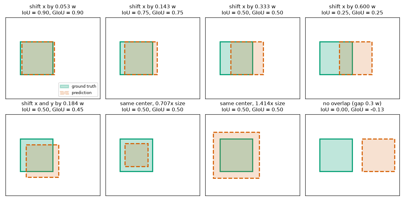
What to read from Figure 2-3:
- Top row (from the left, IoU 0.90, 0.75, 0.50, 0.25): IoU 0.9 looks like a near-perfect match to the eye. 0.75 also looks like a good hit. 0.5 is clearly misaligned but can still be seen as pointing at the same object. 0.25 covers less than half.
- The left three panels of the bottom row all have IoU 0.50: a slight diagonal shift, the same center but smaller, and the same center but larger. Misalignments that look completely different get the same score. IoU does not tell you how a prediction is wrong.
- The rightmost panel of the bottom row: with no overlap, IoU is 0. It is 0 whether the box sits right next to the target or on the opposite side of the image. This weakness is the subject of the latter part of this chapter.
Why small boxes are at a disadvantage
Looking again at \(\operatorname{IoU} = (w - d)/(w + d)\), what determines IoU is not the offset \(d\) itself but its ratio to the width, \(d/w\) (dividing numerator and denominator by \(w\) gives \(\frac{1 - d/w}{1 + d/w}\)). So the same 2-pixel error is negligible for a large box but fatal for a small one. The last table of the earlier output is reproduced below.
| Side of the square box | 2-pixel horizontal offset | 2-pixel offset both horizontally and vertically |
| 80 pixels | IoU 0.9512 | IoU 0.9059 |
| 40 pixels | IoU 0.9048 | IoU 0.8223 |
| 20 pixels | IoU 0.8182 | IoU 0.6807 |
| 10 pixels | IoU 0.6667 | IoU 0.4706 |
| 5 pixels | IoU 0.4286 | IoU 0.2195 |
A box 10 pixels on a side drops to IoU 0.4706 with just a 2-pixel diagonal error, failing to reach the 0.5 threshold. The same error on an 80-pixel box gives 0.9059. This can be checked by hand: for a horizontal-only shift, \(\frac{10 - 2}{10 + 2} = \frac{8}{12} = 0.6667\) and \(\frac{80 - 2}{80 + 2} = \frac{78}{82} = 0.9512\).
Detectors score lower on small objects for many reasons (a major one is that few pixels carry little information to begin with), but the fact that IoU, the scoring yardstick, is this strict on small boxes is one of them. Keep this table in mind when Chapter 3 reports separate scores for small, medium, and large objects (APS, APM, APL). As seen earlier in the shapes world, merely snapping to the pixel grid lowered IoU to 0.9440–0.9795.
Computing all pairs with tensors
The IoU of two boxes can now be computed by hand. But a detector outputs tens to hundreds of predicted boxes per image, and there are several ground-truth boxes as well. Matching in Chapter 7 needs an IoU table of every prediction × every ground truth. With \(N\) predictions and \(M\) ground truths, that is \(N \times M\) IoUs. Running this with two nested Python for loops is slow. With PyTorch broadcasting, it is computed in one go, without loops.
def box_iou(boxes1: torch.Tensor, boxes2: torch.Tensor):
    """모든 쌍의 IoU. boxes1: (N, 4), boxes2: (M, 4), 둘 다 (x0, y0, x1, y1).

    돌려주는 값: iou (N, M), union (N, M). [i, j] 가 boxes1[i] 와 boxes2[j] 의 값이다.
    """
    area1 = box_area(boxes1)  # (N,)
    area2 = box_area(boxes2)  # (M,)
    # 교집합 사각형: 왼쪽 위는 두 박스의 왼쪽 위 가운데 큰 값, 오른쪽 아래는 작은 값
    # boxes1[:, None, :2] 는 (N, 1, 2), boxes2[None, :, :2] 는 (1, M, 2) → 브로드캐스팅으로 (N, M, 2)
    left_top = torch.max(boxes1[:, None, :2], boxes2[None, :, :2])  # (N, M, 2)
    right_bottom = torch.min(boxes1[:, None, 2:], boxes2[None, :, 2:])  # (N, M, 2)
    wh = (right_bottom - left_top).clamp(min=0)  # 겹치지 않으면 음수 → 0 으로 자른다
    inter = wh[..., 0] * wh[..., 1]  # (N, M)
    union = area1[:, None] + area2[None, :] - inter  # (N, 1) + (1, M) − (N, M) → (N, M)
    return inter / union, union
Broadcasting step by step
Broadcasting is the rule that, when operating on two tensors of different shapes, stretches any axis of length 1 to match the other tensor's length, as if it were copied. The rule fits in two lines.
- Line up the shapes of the two tensors from the right end and compare them axis by axis.
- If the axis lengths are equal, leave them as they are; if one is 1, stretch it to the other's length. Otherwise, it is an error.
Let's follow the key line of box_iou, torch.max(boxes1[:, None, :2], boxes2[None, :, :2]), by shape. boxes1 is (N, 4) and boxes2 is (M, 4).
| Step | Expression | Shape | Meaning |
| 1 | | | The first two numbers \((x_0, y_0)\) of each box, i.e., its top-left corner |
| 2 | | | Inserts an axis of length 1 at the |
| 3 | | | This time, an axis of length 1 at the front, leaving the "prediction" axis empty |
| 4 | | | Compare from the right: 2 and 2 are equal, 1 and M become M, N and 1 become N |
Position [i, j] of the result holds the larger of the top-left corners of boxes1[i] and boxes2[j], that is, the top-left corner of their intersection rectangle. All \(N \times M\) pairs are built at once. The remaining lines work the same way.
-
right_bottom: theminof the last two numbers \((x_1, y_1)\). Shape(N, M, 2). -
wh = (right_bottom - left_top).clamp(min=0): (horizontal overlap, vertical overlap) for each pair. Shape(N, M, 2). Clamped to 0 before multiplying. -
inter = wh[..., 0] * wh[..., 1]: multiplies the two numbers in the last axis to get the intersection area. Shape(N, M)....means "keep the leading axes as they are." -
union = area1[:, None] + area2[None, :] - inter:(N, 1) + (1, M) − (N, M)→(N, M). This is inclusion–exclusion. -
inter / union: the IoU table, of shape(N, M). The union is returned as well so it can be reused in the GIoU computation.
Let's print the actual shapes with 3 predictions and 2 ground truths. The first prediction and the first ground truth are our \(A\) and \(B\).
def broadcast_example() -> None:
    """모든 쌍 계산의 모양을 한 단계씩 찍어 본다. 예측 3개 × 정답 2개."""
    preds = torch.tensor([[1.0, 1.0, 5.0, 4.0], [3.0, 2.0, 7.0, 6.0], [8.0, 8.0, 9.0, 9.0]])  # (N = 3, 4)
    targets = torch.tensor([[3.0, 2.0, 7.0, 6.0], [0.0, 0.0, 4.0, 4.0]])  # (M = 2, 4)
    a = preds[:, None, :2]  # (3, 1, 2): 예측마다의 왼쪽 위 (x0, y0). 가운데에 길이 1 인 축을 끼웠다
    b = targets[None, :, :2]  # (1, 2, 2): 정답마다의 왼쪽 위. 맨 앞에 길이 1 인 축을 끼웠다
    left_top = torch.max(a, b)  # 길이 1 인 축이 상대의 길이만큼 늘어난다 → (3, 2, 2)
    print("[4] 모든 쌍 계산의 모양")
    print(f"  preds {tuple(preds.shape)}, targets {tuple(targets.shape)}")
    print(f"  preds[:, None, :2] {tuple(a.shape)}  vs  targets[None, :, :2] {tuple(b.shape)}  →  max {tuple(left_top.shape)}")
    iou, _ = box_iou(preds, targets)
    giou = generalized_box_iou(preds, targets)
    print(f"  IoU  (3, 2) =\n{iou}")
    print(f"  GIoU (3, 2) =\n{giou}")
    # 짝끼리: 예측 k 와 정답 k 만. 여기서는 앞의 두 예측을 두 정답과 짝지었다
    print(f"  짝끼리 IoU (2,) = {paired_box_iou(preds[:2], targets)}  (= 위 행렬의 [0, 0], [1, 1])")
[4] 모든 쌍 계산의 모양
  preds (3, 4), targets (2, 4)
  preds[:, None, :2] (3, 1, 2)  vs  targets[None, :, :2] (1, 2, 2)  →  max (3, 2, 2)
  IoU  (3, 2) =
tensor([[0.1667, 0.4737],
        [1.0000, 0.0667],
        [0.0000, 0.0000]])
  GIoU (3, 2) =
tensor([[-0.0333,  0.4237],
        [ 1.0000, -0.2190],
        [-0.5952, -0.7901]])
  짝끼리 IoU (2,) = tensor([0.1667, 0.0667])  (= 위 행렬의 [0, 0], [1, 1])
Let's read the IoU table. Rows are predictions and columns are ground truths.
-
[0, 0]= 0.1667: the \(\operatorname{IoU}(A, B)\) computed by hand. -
[1, 0]= 1.0000: the second prediction is exactly the same box, \((3, 2, 7, 6)\), as the first ground truth, so it is 1. -
[0, 1]= 0.4737: \(A = (1, 1, 5, 4)\) and the ground truth \((0, 0, 4, 4)\). The intersection is \(\min(5, 4) - \max(1, 0) = 3\) horizontally and \(\min(4, 4) - \max(1, 0) = 3\) vertically, so 9; the union is \(12 + 16 - 9 = 19\); and IoU is \(9/19 = 0.4737\). It checks out. -
[2, 0],[2, 1]= 0: the third prediction \((8, 8, 9, 9)\) overlaps neither ground truth.
All pairs versus paired
IoU is computed in two kinds of situations, and each needs a differently shaped computation.
| All pairs ( | Paired ( | |
| Input | | |
| Output | | |
| When | When it is not yet known which box goes with which: matching cost (Chapter 7), comparing predictions with ground truths during scoring (Chapter 3), NMS (Chapter 3) | When the pairs are already decided: box loss for matched pairs (Chapters 7 and 11), classification losses that use IoU as the target (Chapters 9–11) |
| Amount of computation | \(N \times M\) pairs | \(K\) pairs |
def paired_box_iou(boxes1: torch.Tensor, boxes2: torch.Tensor) -> torch.Tensor:
    """짝지어진 박스끼리의 IoU. boxes1, boxes2: (K, 4) (x0, y0, x1, y1) → (K,). k 번째끼리만 계산한다."""
    left_top = torch.max(boxes1[:, :2], boxes2[:, :2])  # (K, 2): 새 축을 끼우지 않으니 같은 줄끼리만 만난다
    right_bottom = torch.min(boxes1[:, 2:], boxes2[:, 2:])
    wh = (right_bottom - left_top).clamp(min=0)
    inter = wh[:, 0] * wh[:, 1]
    union = box_area(boxes1) + box_area(boxes2) - inter
    return inter / union


def paired_generalized_box_iou(boxes1: torch.Tensor, boxes2: torch.Tensor) -> torch.Tensor:
    """짝지어진 박스끼리의 GIoU (K,). 손실을 계산할 때는 매칭된 쌍만 필요하므로 이 함수를 쓴다."""
    left_top = torch.max(boxes1[:, :2], boxes2[:, :2])
    right_bottom = torch.min(boxes1[:, 2:], boxes2[:, 2:])
    wh = (right_bottom - left_top).clamp(min=0)
    inter = wh[:, 0] * wh[:, 1]
    union = box_area(boxes1) + box_area(boxes2) - inter
    iou = inter / union
    outer_left_top = torch.min(boxes1[:, :2], boxes2[:, :2])
    outer_right_bottom = torch.max(boxes1[:, 2:], boxes2[:, 2:])
    outer_wh = (outer_right_bottom - outer_left_top).clamp(min=0)
    enclosing = outer_wh[:, 0] * outer_wh[:, 1]
    return iou - (enclosing - union) / enclosing
The paired version does not insert axes with None. boxes1[:, :2] and boxes2[:, :2] are both (K, 2), so only rows at the same index meet. The result equals the diagonal of the all-pairs table: the paired IoU values 0.1667 and 0.0667 in the output above are the same as [0, 0] and [1, 1] of the table. Building the whole table and taking its diagonal gives the same answer, but with 300 predictions and 300 ground truths, it would compute 90,000 pairs only to use 300 of them.
Caution: silent failures. If you forget None when computing all pairs, you end up comparing (N, 2) with (M, 2). If \(N \ne M\), an error is raised and you notice right away. But if \(N = M\) by coincidence, it silently computes paired values instead. A result that should be (N, N) comes out as (N,). When writing tensor code, the habit of printing result shapes now and then catches mistakes like this.
Verifying the implementation
Every exercise from Chapter 3 onward uses these functions. A mistake here would break everything after it, so let's verify them in two ways.
- Property checks: on 1,000 pairs of random boxes, check that the properties derived earlier (range, symmetry, 1 with itself, scale invariance) also hold numerically.
- Cross-checking with another method: without using the formula, paint integer-coordinate boxes on a grid and count the cells one by one to obtain the intersection and union. It is like having the computer do the cell counting done by hand in Figure 2-2.
def random_boxes(n: int, generator: torch.Generator) -> torch.Tensor:
    """0 – 1 안에 들어가는 무작위 박스 n 개. (n, 4) (x0, y0, x1, y1)."""
    wh = torch.rand(n, 2, generator=generator) * 0.5 + 0.02  # 너비 · 높이 0.02 – 0.52
    center = wh / 2 + torch.rand(n, 2, generator=generator) * (1 - wh)  # 박스가 그림 밖으로 나가지 않게
    return box_cxcywh_to_xyxy(torch.cat([center, wh], dim=-1))


def check_properties(n: int, generator: torch.Generator) -> None:
    """무작위 박스 n 쌍으로 IoU · GIoU 의 성질을 확인한다. 본문에서 유도한 성질이 숫자로도 맞는지 본다."""
    a, b = random_boxes(n, generator), random_boxes(n, generator)
    a, b = a.double(), b.double()  # 부동소수점 오차를 줄이려고 배정밀도로
    iou = paired_box_iou(a, b)
    giou = paired_generalized_box_iou(a, b)
    all_iou, _ = box_iou(a, b)  # (n, n)
    all_giou = generalized_box_iou(a, b)
    print(f"[5] 무작위 박스 {n}쌍으로 성질 확인")
    print(f"  겹치는 쌍 {int((iou > 0).sum())}개, 겹치지 않는 쌍 {int((iou == 0).sum())}개")
    print(f"  IoU 범위  [{iou.min().item():.4f}, {iou.max().item():.4f}]  → 0 이상 1 이하: {bool((iou >= 0).all() and (iou <= 1).all())}")
    print(f"  GIoU 범위 [{giou.min().item():.4f}, {giou.max().item():.4f}]  → −1 초과 1 이하: {bool((giou > -1).all() and (giou <= 1).all())}")
    print(f"  GIoU ≤ IoU: {bool((giou <= iou + 1e-12).all())}   (IoU − GIoU 의 최솟값 {(iou - giou).min().item():.2e})")
    print(f"  대칭 IoU(A, B) = IoU(B, A): 최대 차 {(iou - paired_box_iou(b, a)).abs().max().item():.1e}"
          f",  GIoU 최대 차 {(giou - paired_generalized_box_iou(b, a)).abs().max().item():.1e}")
    print(f"  자기 자신과는 1: IoU {paired_box_iou(a, a).min().item():.4f}, GIoU {paired_generalized_box_iou(a, a).min().item():.4f}")
    print(f"  짝끼리 = 모든 쌍 행렬의 대각선: 최대 차 IoU {(all_iou.diagonal() - iou).abs().max().item():.1e}"
          f", GIoU {(all_giou.diagonal() - giou).abs().max().item():.1e}")
    scale = torch.tensor([640.0, 480.0, 640.0, 480.0], dtype=torch.float64)  # 가로 640, 세로 480 픽셀로
    print(f"  크기 불변 (가로 640배, 세로 480배): 최대 차 IoU {(paired_box_iou(a * scale, b * scale) - iou).abs().max().item():.1e}"
          f", GIoU {(paired_generalized_box_iou(a * scale, b * scale) - giou).abs().max().item():.1e}")
    back = box_cxcywh_to_xyxy(box_xyxy_to_cxcywh(a))
    print(f"  표현을 바꿨다 되돌리기: 최대 차 {(back - a).abs().max().item():.1e}")


def check_pixel_counting(n: int, generator: torch.Generator, grid: int = 32) -> None:
    """공식을 쓰지 않는 다른 방법과 대조: 정수 좌표 박스를 grid × grid 모눈에 칠하고 칸을 하나하나 센다."""
    low = torch.randint(0, grid - 1, (2, n, 2), generator=generator)  # 왼쪽 위 (x0, y0)
    size = torch.randint(1, grid // 2, (2, n, 2), generator=generator)  # 너비 · 높이 (1 이상)
    boxes = torch.cat([low, (low + size).clamp(max=grid)], dim=-1).float()  # (2, n, 4)
    a, b = boxes[0], boxes[1]
    cells = torch.arange(grid).float() + 0.5  # 칸의 중심 좌표 0.5, 1.5, …

    def paint(box):  # (n, 4) → (n, grid, grid) bool. 칸의 중심이 박스 안이면 True
        inside_x = (cells[None, :] > box[:, 0:1]) & (cells[None, :] < box[:, 2:3])  # (n, grid)
        inside_y = (cells[None, :] > box[:, 1:2]) & (cells[None, :] < box[:, 3:4])
        return inside_y[:, :, None] & inside_x[:, None, :]

    mask_a, mask_b = paint(a), paint(b)
    inter = (mask_a & mask_b).sum(dim=(1, 2)).float()  # 둘 다 칠한 칸 수
    union = (mask_a | mask_b).sum(dim=(1, 2)).float()  # 하나라도 칠한 칸 수
    # 둘러싸는 박스 C: 칠해진 칸이 있는 열 · 행의 범위
    either = mask_a | mask_b
    cols, rows = either.any(dim=1), either.any(dim=2)  # (n, grid)
    # (두 박스 사이에 틈이 있으면 칠해진 열 · 행의 개수가 아니라 처음과 끝 사이의 범위를 써야 한다)
    first_col, last_col = cols.float().argmax(dim=1), grid - 1 - cols.flip(1).float().argmax(dim=1)
    first_row, last_row = rows.float().argmax(dim=1), grid - 1 - rows.flip(1).float().argmax(dim=1)
    enclosing = ((last_col - first_col + 1) * (last_row - first_row + 1)).float()
    count_iou = inter / union
    count_giou = count_iou - (enclosing - union) / enclosing
    print(f"[5] 칸 세기와 대조 ({grid}×{grid} 모눈, 정수 좌표 박스 {n}쌍)")
    print(f"  IoU 최대 차 {(count_iou - paired_box_iou(a, b)).abs().max().item():.1e}"
          f",  GIoU 최대 차 {(count_giou - paired_generalized_box_iou(a, b)).abs().max().item():.1e}")
[5] 무작위 박스 1000쌍으로 성질 확인
  겹치는 쌍 333개, 겹치지 않는 쌍 667개
  IoU 범위  [0.0000, 0.6341]  → 0 이상 1 이하: True
  GIoU 범위 [-0.9810, 0.6196]  → −1 초과 1 이하: True
  GIoU ≤ IoU: True   (IoU − GIoU 의 최솟값 0.00e+00)
  대칭 IoU(A, B) = IoU(B, A): 최대 차 0.0e+00,  GIoU 최대 차 0.0e+00
  자기 자신과는 1: IoU 1.0000, GIoU 1.0000
  짝끼리 = 모든 쌍 행렬의 대각선: 최대 차 IoU 0.0e+00, GIoU 0.0e+00
  크기 불변 (가로 640배, 세로 480배): 최대 차 IoU 1.1e-16, GIoU 2.4e-16
  표현을 바꿨다 되돌리기: 최대 차 0.0e+00
[5] 칸 세기와 대조 (32×32 모눈, 정수 좌표 박스 1000쌍)
  IoU 최대 차 0.0e+00,  GIoU 최대 차 0.0e+00
- Of the 1,000 random pairs, only 333 overlap. Two boxes placed at random are more often apart than not. The predictions of a detector that has just started training are in a similar situation.
- IoU always lies between 0 and 1, swapping the order makes a difference of 0, IoU with itself is 1, and the paired computation differs from the diagonal of the all-pairs table by 0.
- Stretching by 640× horizontally and 480× vertically (converting normalized coordinates to 640×480 pixels) changes IoU only on the order of \(10^{-16}\), that is, by floating-point rounding error alone.
- The difference between cell counting and the formula is exactly 0 for both IoU and GIoU.
The lines about GIoU (range, GIoU ≤ IoU) are revisited after GIoU is introduced.
Box regression loss 1: L1 distance
So far we have compared two boxes. Now let's change perspective and think about fitting a predicted box to a ground-truth box. Neural network training runs in the following order (it is covered from scratch in Chapter 4; for now, it is enough to grasp three terms).
- Loss: a single number measuring how wrong a prediction is compared with the ground truth. Smaller is better, and a perfect prediction gives 0. The formula that computes the loss is called the loss function.
- Gradient: how much the loss changes when the prediction changes very slightly (the derivative). It is a compass that tells you which way to move to reduce the loss.
- Gradient descent (see Gradient descent): a method that reduces the loss by repeatedly taking small steps in the direction opposite to the gradient.
Predicting continuous values such as the four numbers of a box is called regression, and predicting boxes is called box regression. The rest of this chapter is about which loss to use for box regression. The ground-truth box is written \(b\) and the predicted box \(\hat{b}\) ("b hat"; the hat marks a value predicted by the model). Both are in normalized center format.
\(b = (c_x,\ c_y,\ w,\ h), \qquad \hat{b} = (\hat{c}_x,\ \hat{c}_y,\ \hat{w},\ \hat{h})\)
Definition of L1 distance and a hand calculation
The first approach that comes to mind is to compare the four numbers one by one and add up the differences.
\(\mathcal{L}_{\text{L1}}(b, \hat{b}) = \|b - \hat{b}\|_1 = |c_x - \hat{c}_x| + |c_y - \hat{c}_y| + |w - \hat{w}| + |h - \hat{h}|\)
This is the L1 distance, and when used as a loss it is called the L1 loss. \(\mathcal{L}\) is a script L standing for loss, and \(\|\cdot\|_1\) is the notation for "take the absolute value of each component and sum them" (the L1 norm). Let's compute it for our example. Converting \(A\) and \(B\) to center format gives \((3, 2.5, 4, 3)\) and \((5, 4, 4, 4)\), so
\(\|A - B\|_1 = |3 - 5| + |2.5 - 4| + |4 - 4| + |3 - 4| = 2 + 1.5 + 0 + 1 = 4.5\)
This matches the L1 value of 4.5 in the earlier output. It is 0 when the two boxes are identical and grows as they differ. Note also that it has a well-defined value whether or not the boxes overlap.
Why not L2?
Instead of absolute values, differences can also be measured with squares, as in the L2 loss (squared error) \(\sum (\text{difference})^2\). The reason the L1 family is more widely used for box regression becomes clear when the gradients are compared. Let \(e\) be the error in one coordinate (e.g., \(e = \hat{c}_x - c_x\)).
| Loss | Gradient (derivative of the loss with respect to \(e\)) | Gradient at \(e = 0.01\) | Gradient at \(e = 0.5\) | |
| L1 | \(|e|\) | \(+1\) if \(e \gt 0\), \(-1\) if \(e \lt 0\) | 1 | 1 |
| L2 | \(e^2\) | \(2e\) | 0.02 | 1.0 |
- L2 gets dragged around by badly wrong predictions. Its gradient is proportional to the error, so one box with an error of 0.5 pulls the model as hard as 50 boxes with an error of 0.01. Early in training, predictions often land in odd places, and a handful of such outliers (values that deviate unusually far) end up dominating training.
- The L1 gradient always has magnitude 1. It pulls with the same force whether the error is large or small, so it is less swayed by outliers. In its review of related work, the GIoU paper also notes that Fast R-CNN proposed the smooth L1 loss (L1 smoothed out near 0) to make training more robust to outliers.
- There is a price. The L1 gradient does not shrink even right next to the target. Even after arriving, it keeps trying to move with the same step size as at the start, so unless the step size (learning rate) is reduced, it oscillates around the target. A later experiment shows this directly. Also, at the single point \(e = 0\) the graph has a sharp corner and the derivative is undefined (PyTorch returns 0 there).
The weakness of L1: dependence on size
L1 has a more fundamental problem: it does not know the size of the box. We saw earlier that the same error of 0.05 is trivial for a large box and fatal for a small one, yet L1 gives both the same value.
| Ground-truth box (normalized) | Prediction | L1 distance | IoU |
| Large box: width and height 0.5 | Only the center is off by 0.05 horizontally | 0.05 | \(\dfrac{0.5 - 0.05}{0.5 + 0.05} = 0.8182\) |
| Small box: width and height 0.1 | Only the center is off by 0.05 horizontally | 0.05 | \(\dfrac{0.1 - 0.05}{0.1 + 0.05} = 0.3333\) |
L1 is 0.05 in both cases, but by IoU, the scoring yardstick, they score 0.8182 and 0.3333. One is an excellent prediction and the other a failure. Trained with the L1 loss alone, a model concentrates on large boxes, where it can reduce the loss a lot, and treats the "small but fatal" errors on small boxes lightly.
The DETR paper (Section 3.1) points out the same problem: when boxes are predicted directly, the relative scaling of the loss becomes an issue, because the L1 loss has different scales for small and large boxes even when their relative errors are similar. Figure 1 of the GIoU paper likewise shows three pairs of boxes with the same L1 distance of 9.07 but different IoUs of 0.27, 0.59, and 0.66. Since what we really want to increase is IoU, the idea of using IoU itself as the loss follows naturally.
Box regression loss 2: IoU loss and the flat plain
IoU loss
IoU should be large while a loss should be small, so subtract IoU from 1.
\(\mathcal{L}_{\operatorname{IoU}}(b, \hat{b}) = 1 - \operatorname{IoU}(b, \hat{b})\)
This is the IoU loss. It is 0 for a perfect match and 1 when there is no overlap at all. Since IoU is scale invariant, so is this loss: it gives the same value for the same degree of misalignment in large and small boxes. The weakness of L1 is gone. But a new, more serious problem appears.
No overlap means zero gradient
Let's look again at the IoU of the "box shifted horizontally by \(d\)" as a function of \(d\). This time, include the case where \(d\) exceeds \(w\) and the two boxes are completely separated.
- Gradient of the IoU loss with respect to the horizontal shift \(d\)
- \(\operatorname{IoU}(d) = \begin{cases} \dfrac{w - d}{w + d} & 0 \le d \lt w \quad (\text{overlap}) \\ 0 & d \ge w \quad (\text{no overlap}) \end{cases}\). For \(d \lt w\), this is the formula derived earlier. For \(d \ge w\), the horizontal overlap \(w - d\) is 0 or less, so it is clamped to 0; the intersection is 0, and so is IoU. The brace means "different formulas depending on the case."
- \(\frac{d}{dd}\,\frac{w - d}{w + d} = \frac{(-1)(w + d) - (w - d)(1)}{(w + d)^2}\). Differentiate with respect to \(d\) over the overlapping range, plugging \(f = w - d\) (\(f' = -1\)) and \(g = w + d\) (\(g' = 1\)) into the quotient rule \(\left(\frac{f}{g}\right)' = \frac{f'g - fg'}{g^2}\). The leading \(\frac{d}{dd}\) is notation for "differentiate with respect to \(d\)."
- \(= \frac{-w - d - w + d}{(w + d)^2} = -\frac{2w}{(w + d)^2}\). Expanding the numerator, \(d\) cancels and \(-2w\) remains. It is negative, meaning "the more you shift, the lower the IoU."
- \(\frac{d\,\mathcal{L}_{\operatorname{IoU}}}{dd} = -\frac{d\,\operatorname{IoU}}{dd} = \begin{cases} \dfrac{2w}{(w + d)^2} & 0 \lt d \lt w \\ 0 & d \gt w \end{cases}\). The loss is \(1 - \operatorname{IoU}\), so only the sign flips. While the boxes overlap, the gradient is positive, giving the signal "decrease \(d\) (move toward the target)." But once they separate, IoU is the constant 0, so its derivative is 0 too.
Let's check with numbers. If a box with \(w = 2\) is shifted by \(d = 1\), then \(\operatorname{IoU} = \frac{2 - 1}{2 + 1} = \frac{1}{3}\), the loss is \(0.6667\), and the gradient is \(\frac{2 \cdot 2}{(2 + 1)^2} = \frac{4}{9} = 0.4444\). With \(d = 3\), a gap of 1 opens between the boxes; IoU is 0, the loss is 1, and the gradient is 0. Whether \(d = 3\) or \(d = 300\), the loss is 1 and the gradient is 0 all the same.
Imagine making your way down to the bottom of a valley in thick fog. All you can do is feel the slope underfoot and head downhill. On a slope that works fine, but in the middle of a wide, flat plain there is no way to tell which way the valley lies. The IoU loss for non-overlapping boxes is exactly that plain. The loss is high at 1 (far from the valley), yet the ground underfoot is perfectly flat (zero gradient) and gives no direction to move in.
This is not rare. Just earlier, 667 of the 1,000 random box pairs did not overlap. At the start of training, predicted boxes often do not overlap the ground truth, and with the IoU loss alone such boxes never move. The GIoU paper calls this the "plateau" of IoU and notes that the gradient of IoU is 0 in every non-overlapping case.
GIoU: overlap you can see even when boxes are apart
What is needed is a value that keeps the strengths of IoU (scale invariance, a clean 0–1 scale) while reflecting how far apart the boxes are even when they do not overlap. The answer is GIoU (Generalized Intersection over Union, read "G-I-o-U"), proposed by Rezatofighi et al. in the 2019 paper "Generalized Intersection over Union: A Metric and A Loss for Bounding Box Regression."
The enclosing box
GIoU brings in one more box. Let \(C\) be the smallest box that covers both \(A\) and \(B\). This chapter calls it the enclosing box (smallest enclosing box). The formula for \(C\) uses max and min in exactly the opposite way from the intersection: to cover both boxes, the top-left corner must be further left and up (smaller values), and the bottom-right corner further right and down (larger values).
\(C = \big(\min(x_0^A, x_0^B),\ \ \min(y_0^A, y_0^B),\ \ \max(x_1^A, x_1^B),\ \ \max(y_1^A, y_1^B)\big)\)
Besides \(A\) and \(B\), \(C\) may contain empty space that belongs to neither box. Its area is \(|C| - |A \cup B|\). The more misaligned or the farther apart the two boxes are, the larger this empty space becomes. GIoU subtracts the fraction of this empty space from IoU.
Figure 2-4 in the original draws the enclosing box \(C = (1, 1, 7, 6)\) as a dashed line over \(A\) and \(B\) from Figure 2-2, and lightly shades the empty space inside \(C\) that belongs to neither \(A\) nor \(B\). \(C\)'s left = \(\min(1, 3) = 1\), top = \(\min(1, 2) = 1\), right = \(\max(5, 7) = 7\), and bottom = \(\max(4, 6) = 6\); the area of \(C\) is \(6 \times 5 = 30\) and the union is 24, so the empty space is \(30 - 24 = 6\). Two cells at the top right and four at the bottom left, six in all, belong to neither box.
Definition of GIoU and a hand calculation
\(\operatorname{GIoU}(A, B) = \operatorname{IoU}(A, B) - \frac{|C| - |A \cup B|}{|C|}\)
The second term is the fraction of \(C\) that is empty, a penalty between 0 and 1. If the two boxes fill \(C\) with no gaps, the penalty is 0 and GIoU equals IoU; the more empty space there is, the further GIoU falls below IoU. Let's compute the example in Figure 2-4 by hand.
- GIoU of \(A = (1, 1, 5, 4)\) and \(B = (3, 2, 7, 6)\)
- \(|A \cap B| = 4, \qquad |A \cup B| = 24, \qquad \operatorname{IoU} = \frac{4}{24} = \frac{1}{6}\). These are the values found earlier.
- \(C = \big(\min(1, 3),\ \min(1, 2),\ \max(5, 7),\ \max(4, 6)\big) = (1, 1, 7, 6)\). The enclosing box: the top-left corner takes the smaller values, the bottom-right corner the larger.
- \(|C| = (7 - 1)(6 - 1) = 6 \times 5 = 30\). The area of \(C\).
- \(\frac{|C| - |A \cup B|}{|C|} = \frac{30 - 24}{30} = \frac{6}{30} = 0.2\). The empty space is 6 cells, 20% of \(C\). This is the penalty.
- \(\operatorname{GIoU}(A, B) = \frac{1}{6} - \frac{6}{30} = 0.1667 - 0.2 = -0.0333\). Subtract the penalty from IoU. The result is negative, matching the GIoU of −0.0333 in the earlier code output.
def generalized_box_iou(boxes1: torch.Tensor, boxes2: torch.Tensor) -> torch.Tensor:
    """모든 쌍의 GIoU (N, M). GIoU = IoU − (C 의 넓이 − 합집합) / C 의 넓이. C 는 두 박스를 모두 덮는 가장 작은 박스."""
    iou, union = box_iou(boxes1, boxes2)
    # 둘러싸는 박스 C: 왼쪽 위는 작은 값, 오른쪽 아래는 큰 값 (교집합과 max · min 이 정확히 반대)
    left_top = torch.min(boxes1[:, None, :2], boxes2[None, :, :2])
    right_bottom = torch.max(boxes1[:, None, 2:], boxes2[None, :, 2:])
    wh = (right_bottom - left_top).clamp(min=0)
    enclosing = wh[..., 0] * wh[..., 1]
    return iou - (enclosing - union) / enclosing
The code takes the IoU and union returned by box_iou and computes only one more thing, the area of the enclosing box, enclosing. The positions of min and max are swapped relative to box_iou. Broadcasting works the same way: (N, 1, 2) against (1, M, 2) → (N, M, 2). The GIoU table entry [2, 0] = −0.5952 in the earlier all-pairs output can also be checked by hand. The prediction \((8, 8, 9, 9)\) and the ground truth \((3, 2, 7, 6)\) do not overlap, so IoU is 0 and the union is \(1 + 16 = 17\); \(C = (3, 2, 9, 9)\) has area \(6 \times 7 = 42\); therefore \(\operatorname{GIoU} = 0 - \frac{42 - 17}{42} = -0.5952\).
Properties of GIoU
Rewriting the definition slightly makes its properties visible at a glance. Splitting the penalty term gives \(\frac{|C| - |A \cup B|}{|C|} = 1 - \frac{|A \cup B|}{|C|}\), so
\(\operatorname{GIoU}(A, B) = \underbrace{\frac{|A \cap B|}{|A \cup B|}}_{\operatorname{IoU}:\ \text{between } 0 \text{ and } 1} + \underbrace{\frac{|A \cup B|}{|C|}}_{\text{greater than } 0,\ \text{at most } 1} - 1\)
The second term is the fraction of \(C\) filled by the two boxes. The following properties follow from this form.
- Four properties of GIoU
- \(|A \cup B| \le |C| \quad\Longrightarrow\quad \frac{|C| - |A \cup B|}{|C|} \ge 0 \quad\Longrightarrow\quad \operatorname{GIoU}(A, B) \le \operatorname{IoU}(A, B)\). GIoU cannot exceed IoU. \(C\) covers both boxes, so it cannot be smaller than the union, and the penalty is therefore at least 0. Subtracting something nonnegative from IoU leaves at most IoU.
- \(\operatorname{GIoU} = \operatorname{IoU} + \frac{|A \cup B|}{|C|} - 1 \ \gt\ 0 + 0 - 1 = -1, \qquad \operatorname{GIoU} \le \operatorname{IoU} \le 1\). The range is \(-1 \lt \operatorname{GIoU} \le 1\). IoU is at least 0, and for boxes with nonzero area, \(\frac{|A \cup B|}{|C|}\) is greater than 0, so GIoU is greater than \(-1\). The upper bound follows from the previous property. Unlike IoU's range of 0–1, this range is symmetric around 0.
- \(A = B \quad\Longrightarrow\quad C = A,\ \ |A \cup B| = |C| \quad\Longrightarrow\quad \operatorname{GIoU} = 1 + 1 - 1 = 1\). It is 1 when the two boxes are identical. Conversely, if GIoU is 1, then \(\operatorname{IoU} \ge \operatorname{GIoU} = 1\), so IoU is also 1, meaning the boxes are identical. As with IoU, it is 1 only when the boxes are identical.
- \(A \cap B = \varnothing \quad\Longrightarrow\quad \operatorname{GIoU} = \frac{|A| + |B|}{|C|} - 1 \ \longrightarrow\ -1 \quad (\text{as the boxes move infinitely far apart})\). When the boxes do not overlap (\(\varnothing\) is the empty set, indicating that there is no overlap), IoU is 0 and the union is \(|A| + |B|\). As the boxes move apart, \(C\) grows, the first term goes to 0, and GIoU approaches \(-1\). The farther apart, the lower the value: information that IoU did not have.
On top of that, GIoU is scale invariant just like IoU. Multiplying the coordinates by \(k\) scales \(|C|\) by \(k^2\) as well, which cancels between the numerator and denominator of the penalty. These properties match the ones listed in the GIoU paper (the paper writes the range as \(-1 \le \operatorname{GIoU} \le 1\) and explains that \(-1\) is the limit as \(|A \cup B| / |C|\) goes to 0). In the earlier random-box check, GIoU ranged over \([-0.9810,\ 0.6196]\), and GIoU ≤ IoU held for all 1,000 pairs.
Caution: a negative GIoU does not mean the boxes are apart. Our \(A\) and \(B\) clearly overlap (IoU 0.1667), yet GIoU is negative at −0.0333, because the fraction of empty space was larger than that of the overlap. "No overlap implies GIoU ≤ 0" is true, but the converse ("a negative GIoU implies no overlap") is false. Whether boxes overlap should be judged by whether IoU is 0.
When GIoU is used as a loss, it is subtracted from 1, like the IoU loss. This is the GIoU loss.
\(\mathcal{L}_{\operatorname{GIoU}}(b, \hat{b}) = 1 - \operatorname{GIoU}(b, \hat{b}), \qquad 0 \le \mathcal{L}_{\operatorname{GIoU}} \lt 2\)
It is 0 for a perfect match, exceeds 1 once the boxes stop overlapping, and approaches 2 as they move infinitely far apart.
The gradient survives without overlap
Let's compute GIoU for the very example that trapped the IoU loss on the plain: shifting a same-size box horizontally by \(d\).
- GIoU and its gradient with respect to the horizontal shift \(d\)
- \(C = [0,\ w + d] \times [0,\ h], \qquad |C| = (w + d)\,h \qquad (\text{for all } d \ge 0)\). The smallest horizontal interval covering both the target \([0, w]\) and the prediction \([d, w + d]\) is \([0, w + d]\), whether or not they overlap.
- \(0 \le d \lt w: \quad |A \cup B| = (w + d)\,h = |C| \quad\Longrightarrow\quad \operatorname{GIoU} = \operatorname{IoU} = \frac{w - d}{w + d}\). While the boxes overlap, the union fills \(C\) with no gaps (the heights are equal and the shift is purely horizontal). The penalty is 0, so GIoU equals IoU.
- \(d \ge w: \quad \operatorname{IoU} = 0, \quad |A \cup B| = 2wh \quad\Longrightarrow\quad \operatorname{GIoU} = 0 - \frac{(w + d)h - 2wh}{(w + d)h} = -\frac{d - w}{w + d}\). Once the boxes are apart, the intersection is 0, so the union is the sum of the two areas, \(2wh\). The empty space is the gap between the boxes, a rectangle \(d - w\) wide and \(h\) tall. \(h\) cancels.
- \(-\frac{d - w}{w + d} = \frac{w - d}{w + d}\). Tidying up the sign of the numerator gives exactly the same formula, letter for letter, as in the overlapping case. In this arrangement, GIoU is given by the single formula \(\frac{w - d}{w + d}\) over all \(d \ge 0\). Where IoU stopped at 0, GIoU continues along the same curve and goes negative.
- \(\frac{d\,\mathcal{L}_{\operatorname{GIoU}}}{dd} = -\frac{d}{dd}\,\frac{w - d}{w + d} = \frac{2w}{(w + d)^2} \ \gt\ 0 \qquad (\text{for all } d \gt 0)\). The differentiation is the same calculation as for the IoU loss. The difference is that this formula stays valid for \(d \gt w\) as well. No matter how far apart the boxes are, the gradient is not 0 and always points toward "decrease \(d\)."
Plugging in numbers: with \(w = 2\) and \(d = 3\) (a gap of 1), \(\operatorname{GIoU} = \frac{2 - 3}{2 + 3} = -0.2\), the loss is \(1.2\), and the gradient is \(\frac{2 \cdot 2}{(2 + 3)^2} = \frac{4}{25} = 0.16\). Computing from the definition gives the same result: union \(4 + 4 = 8\), \(|C| = 5 \times 2 = 10\), \(\operatorname{GIoU} = 0 - \frac{10 - 8}{10} = -0.2\). However, as the form of the formula shows, the gradient shrinks as \(1/(w + d)^2\) with distance. It is alive, but weak from afar. This point comes up again in the experiments.
Let's verify this hand calculation with PyTorch's automatic differentiation (autograd). Autograd records the computations performed on tensors and computes the derivatives for you when backward() is called (the principle is covered in Chapter 4). The target is \((x_0, y_0, x_1, y_1) = (3, 0, 5, 2)\), and the prediction is a box of the same size placed to its left. Because the prediction is to the left of the target, increasing the prediction's center \(\hat{c}_x\) decreases \(d\). So the gradient with respect to \(\hat{c}_x\) is the value found above with a minus sign.
def box_l1(pred: torch.Tensor, target: torch.Tensor) -> torch.Tensor:
    """L1 거리. pred, target: (K, 4) (cx, cy, w, h) → (K,). 네 숫자의 차의 절댓값을 더한다."""
    return (pred - target).abs().sum(dim=-1)


def iou_loss(pred: torch.Tensor, target: torch.Tensor) -> torch.Tensor:
    """IoU 손실 1 − IoU. pred, target: (K, 4) (cx, cy, w, h) → (K,)."""
    return 1 - paired_box_iou(box_cxcywh_to_xyxy(pred), box_cxcywh_to_xyxy(target))


def giou_loss(pred: torch.Tensor, target: torch.Tensor) -> torch.Tensor:
    """GIoU 손실 1 − GIoU. 값의 범위는 0 (완전히 일치) – 2 (한없이 멀리)."""
    return 1 - paired_generalized_box_iou(box_cxcywh_to_xyxy(pred), box_cxcywh_to_xyxy(target))


def detr_box_loss(pred: torch.Tensor, target: torch.Tensor, l1_coef: float = 5.0, giou_coef: float = 2.0):
    """DETR 계열의 박스 손실 = 5 · L1 + 2 · (1 − GIoU). 계수 5 와 2 는 DETR · LW-DETR · RF-DETR 이 모두 쓰는 값."""
    return l1_coef * box_l1(pred, target) + giou_coef * giou_loss(pred, target)


LOSSES = {  # 이름 → 손실 함수. 실험 · 그림에서 이 순서로 쓴다
    "1 - IoU": iou_loss,
    "1 - GIoU": giou_loss,
    "L1": box_l1,
    "5 L1 + 2 (1 - GIoU)": detr_box_loss,
}
def box_gradient(loss_fn, pred: torch.Tensor, target: torch.Tensor) -> torch.Tensor:
    """손실을 예측 박스 (cx, cy, w, h) 로 미분한 기울기 (4,). autograd 가 계산한다."""
    pred = pred.clone().requires_grad_(True)  # 이 텐서로 미분하겠다고 표시
    loss_fn(pred[None], target[None]).sum().backward()  # 손실 → 역전파
    return pred.grad


def gradient_example() -> None:
    """본문의 손계산과 맞춰 보는 기울기. 정답 T = (3, 0, 5, 2), 예측은 같은 크기(2 × 2)로 왼쪽에 있다."""
    target = box_xyxy_to_cxcywh(torch.tensor([3.0, 0.0, 5.0, 2.0]))  # (cx, cy, w, h) = (4, 1, 2, 2)
    print("[6] autograd 로 본 기울기: 정답 (x0, y0, x1, y1) = (3, 0, 5, 2), 예측은 너비 · 높이 2")
    print("    손실을 예측의 (cx, cy, w, h) 로 미분한 값")
    for name, x0 in [("겹치지 않음 (예측 x0 = 0, d = 3)", 0.0), ("겹침       (예측 x0 = 2, d = 1)", 2.0)]:
        pred = box_xyxy_to_cxcywh(torch.tensor([x0, 0.0, x0 + 2.0, 2.0]))
        print(f"  {name}")
        for loss_name, loss_fn in LOSSES.items():
            value = loss_fn(pred[None], target[None]).item()
            grad = box_gradient(loss_fn, pred, target)
            print(f"    {loss_name:<20} 값 = {value:8.4f}   기울기 = {fmt(grad)}")
[6] autograd 로 본 기울기: 정답 (x0, y0, x1, y1) = (3, 0, 5, 2), 예측은 너비 · 높이 2
    손실을 예측의 (cx, cy, w, h) 로 미분한 값
  겹치지 않음 (예측 x0 = 0, d = 3)
    1 - IoU              값 =   1.0000   기울기 = [0.0000, 0.0000, 0.0000, 0.0000]
    1 - GIoU             값 =   1.2000   기울기 = [-0.1600, 0.0000, -0.1200, 0.0000]
    L1                   값 =   3.0000   기울기 = [-1.0000, 0.0000, 0.0000, 0.0000]
    5 L1 + 2 (1 - GIoU)  값 =  17.4000   기울기 = [-5.3200, 0.0000, -0.2400, 0.0000]
  겹침       (예측 x0 = 2, d = 1)
    1 - IoU              값 =   0.6667   기울기 = [-0.4444, 0.0000, -0.1111, 0.0000]
    1 - GIoU             값 =   0.6667   기울기 = [-0.4444, 0.0000, -0.1111, 0.0000]
    L1                   값 =   1.0000   기울기 = [-1.0000, 0.0000, 0.0000, 0.0000]
    5 L1 + 2 (1 - GIoU)  값 =   6.3333   기울기 = [-5.8889, 0.0000, -0.2222, 0.0000]
The four numbers of each gradient are, in order, the derivatives with respect to the prediction's \((\hat{c}_x, \hat{c}_y, \hat{w}, \hat{h})\).
- IoU loss without overlap: value 1.0000, and the gradient is 0 in all four components. Exactly as derived, it gives no direction to move in at all.
- GIoU loss without overlap: value 1.2000, \(\hat{c}_x\) component −0.1600. These are the hand-calculated \(1.2\) and \(0.16\), with a sign attached (moving right reduces the loss). Gradient descent moves opposite to the gradient, so it increases \(\hat{c}_x\), toward the target.
- The \(\hat{w}\) component, −0.1200, is also worth noting. It means that widening the box also reduces the GIoU loss. This can be checked by hand. Writing the prediction's width as \(\hat{w}\) (with the center fixed at 1), the union is \(2\hat{w} + 4\) and \(|C| = 2\,(4 + \hat{w}/2) = 8 + \hat{w}\), so \(\operatorname{GIoU} = \frac{2\hat{w} + 4}{8 + \hat{w}} - 1\); differentiating with respect to \(\hat{w}\) gives \(\frac{2(8 + \hat{w}) - (2\hat{w} + 4)}{(8 + \hat{w})^2} = \frac{12}{100} = 0.12\) (at \(\hat{w} = 2\)). While the boxes do not overlap, the GIoU loss tries to move the box toward the target and enlarge it at the same time, because enlarging the box reduces the fraction of empty space.
- With overlap: the IoU loss and the GIoU loss have the same value (0.6667) and the same gradient, because in this arrangement the penalty is 0 while the boxes overlap. The \(\hat{c}_x\) component −0.4444 is the hand-calculated \(4/9\).
- L1: the \(\hat{c}_x\) component is −1.0000 whether or not the boxes overlap, a gradient whose magnitude is always 1. The width and height already match the target, so those components are 0.
- The last line,
5 L1 + 2 (1 - GIoU), is the DETR-family box loss explained at the end of this chapter. Its value \(17.4 = 5 \times 3 + 2 \times 1.2\) and gradient \(-5.32 = 5 \times (-1) + 2 \times (-0.16)\) show that it is the two losses multiplied by their coefficients and added together.
Note: why the \(\hat{c}_y\) and \(\hat{h}\) components are 0. In this example, the tops and bottoms of the two boxes are exactly aligned. \(\hat{c}_y\) sits at the midpoint, where moving up or down makes things equally worse, so its component is 0. \(\hat{h}\) sits at a special point where the two arguments of max/min are exactly equal. At such points, PyTorch splits the gradient equally between the two arguments, and in this example the results happen to cancel out to 0. If the heights of the two boxes differed even slightly, a nonzero value would appear. It is enough to know that this comes from the symmetry of this particular example and is not a general phenomenon.
Experiments: shift it, then descend
Let's confirm the derivations with experiments. There are four: ① plotting the curves of the three values while shifting the prediction horizontally, ② plotting the loss surfaces, ③ fitting a single box to the target with gradient descent, and ④ jittering boxes in the shapes world. All of them run with a single python ch02_boxes.py in 8–15 seconds on a CPU (no GPU is used).
Watching three values while shifting horizontally
In normalized coordinates, take a ground-truth box with width and height \(w = 0.2\) and shift a same-size prediction horizontally from \(d = 0\) to \(3w\). At each point, measure L1, IoU, and GIoU, along with the magnitude of each loss's gradient with respect to \(\hat{c}_x\).
def slide_curves(points: int):
    """예측 박스(정답과 같은 크기)를 정답에서 가로로 d 만큼 밀어 가며 L1 · IoU · GIoU 와 손실의 기울기를 잰다.

    돌려주는 값: d (points,), 값 사전, 기울기 사전(손실을 cx 로 미분한 값의 절댓값).
    """
    width, height = 0.2, 0.2
    target = torch.tensor([0.3, 0.5, width, height])  # 정규화 (cx, cy, w, h)
    shifts = torch.linspace(0.0, 3 * width, points)  # d = 0 … 3w
    pred = target.repeat(points, 1)  # (points, 4)
    pred[:, 0] += shifts  # 중심만 오른쪽으로
    pred.requires_grad_(True)
    targets = target.repeat(points, 1)
    values, grads = {}, {}
    for name, loss_fn in list(LOSSES.items())[:3]:
        loss = loss_fn(pred, targets)  # (points,)
        (grad,) = torch.autograd.grad(loss.sum(), pred)  # (points, 4): 점마다 따로 미분된다
        values[name] = loss.detach()
        grads[name] = grad[:, 0].abs()  # cx 방향 성분의 크기
    print("[7] 가로로 밀기 (w = 0.2): 값과 |d손실/dcx|")
    print("    d/w    L1     IoU     GIoU   | 기울기 1−IoU  1−GIoU    L1   | 공식 2w/(w+d)²")
    for ratio in (0.0, 0.1, 0.25, 0.5, 0.9, 1.1, 1.5, 2.0, 3.0):
        k = int(torch.argmin((shifts / width - ratio).abs()))
        d = shifts[k].item()
        print(f"    {d / width:4.2f}  {values['L1'][k].item():.4f}  {1 - values['1 - IoU'][k].item():7.4f} {1 - values['1 - GIoU'][k].item():7.4f}"
              f"  |   {grads['1 - IoU'][k].item():7.4f}  {grads['1 - GIoU'][k].item():7.4f}  {grads['L1'][k].item():.4f} |   {2 * width / (width + d) ** 2:7.4f}")
    return shifts, values, grads
[7] 가로로 밀기 (w = 0.2): 값과 |d손실/dcx|
    d/w    L1     IoU     GIoU   | 기울기 1−IoU  1−GIoU    L1   | 공식 2w/(w+d)²
    0.00  0.0000   1.0000  1.0000  |    0.0000   0.0000  0.0000 |   10.0000
    0.10  0.0200   0.8182  0.8182  |    8.2645   8.2645  1.0000 |    8.2645
    0.25  0.0500   0.6000  0.6000  |    6.4000   6.4000  1.0000 |    6.4000
    0.50  0.1000   0.3333  0.3333  |    4.4444   4.4444  1.0000 |    4.4444
    0.90  0.1800   0.0526  0.0526  |    2.7701   2.7701  1.0000 |    2.7701
    1.10  0.2200   0.0000 -0.0476  |    0.0000   2.2676  1.0000 |    2.2676
    1.50  0.3000   0.0000 -0.2000  |    0.0000   1.6000  1.0000 |    1.6000
    2.00  0.4000   0.0000 -0.3333  |    0.0000   1.1111  1.0000 |    1.1111
    3.00  0.6000   0.0000 -0.5000  |    0.0000   0.6250  1.0000 |    0.6250
- Figure: Figure 2-5. Values and loss gradient magnitudes when shifting the prediction horizontally — the left panel shows IoU, GIoU, and the L1 distance against the shift; the right panel shows the gradient magnitudes of the three losses. The horizontal axis is the shift divided by the box width, \(d/w\), and the two boxes separate at the vertical dashed line (\(d = w\)).
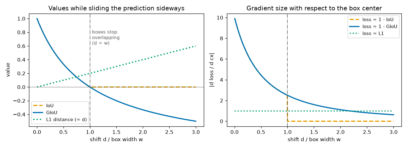
What to read from the table and Figure 2-5:
- Left, IoU and GIoU. For \(d \lt w\), the two curves coincide exactly (the values are equal in the rows \(d/w = 0.10\)–\(0.90\)). At \(d = w\), IoU reaches 0 and stays on the floor, while GIoU continues down the same curve without a kink: −0.0476 at \(d/w = 1.1\), −0.3333 at 2, and −0.5000 at 3. Plugging \(d = 3w\) into \(\frac{w - d}{w + d}\) gives \(\frac{-2w}{4w} = -0.5\).
- Left, L1. A straight line equal to the shift itself (0.2 at \(d = 0.2\)). It has nothing to do with whether the boxes overlap.
- Right, gradient of the IoU loss. The moment \(d\) passes \(w\), it drops abruptly from \(\frac{2w}{(2w)^2} = \frac{1}{2w} = 2.5\) to 0. In the table, it is 2.7701 at \(d/w = 0.90\) and 0.0000 at \(1.10\). This is where the plain begins.
- Right, gradient of the GIoU loss. It passes the same point smoothly, 2.7701 → 2.2676. The values computed by autograd match the formula \(\frac{2w}{(w + d)^2}\) in the last column to four decimal places throughout. But it shrinks with distance: at \(d = 3w\) it is 0.6250, smaller even than L1's constant 1. The two curves cross at \(d \approx 2.2\,w\) (solving \(\frac{2w}{(w+d)^2} = 1\) with \(w = 0.2\) gives \(d = 0.432\)).
- Up close, the GIoU loss gradient is much larger. At \(d/w = 0.1\) it is 8.2645, about eight times L1's. And this magnitude depends on the box size. Writing \(d = r\,w\) gives \(\frac{2w}{(w + rw)^2} = \frac{2}{w\,(1 + r)^2}\), so for the same relative offset \(r\), the smaller the box, the larger the gradient (proportional to \(1/w\)). Penalizing small errors on small boxes heavily is exactly the property L1 lacked.
- The \(d = 0\) row. The formula gives 10, but autograd returns 0. This is not a mistake. \(d = 0\) is the sharp corner where the loss is lowest; moving left or right both increase the loss. The derivative is not uniquely defined there, and PyTorch returns 0 at such points. The formula's 10 is the gradient when approaching from the right.
Loss surfaces
This time, fix the size of the predicted box to that of the target and move its center \((\hat{c}_x, \hat{c}_y)\) across the whole image. Coloring the loss value at each center position gives a loss surface. Gradient descent behaves like a marble placed on this surface, rolling in the steepest downhill direction from wherever it is.
- Figure: Figure 2-6. Loss surfaces when moving the center of the predicted box — from the left, \(1 - \operatorname{IoU}\), \(1 - \operatorname{GIoU}\), and L1. The white dashed line is the ground-truth box, the white cross is its center, and the white solid lines are contour lines (points of equal loss). Darker means lower loss.
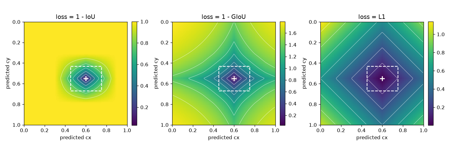
- \(1 - \operatorname{IoU}\) (left): only a narrow area around the target is sunken; everything else is a yellow plain with loss 1. Contour lines appear only near the target. A marble on the plain does not roll. If the prediction's center is at least \(w\) away horizontally or at least \(h\) away vertically from the target, it is on this plain.
- \(1 - \operatorname{GIoU}\) (center): there is no plain. From every corner of the image, the contour lines surround the target, so wherever the marble is placed, it rolls toward the target. A cross-shaped valley is visible: when either the horizontal or the vertical position lines up with the target, the empty space shrinks and the loss drops. The color scale goes above 1, up to around 1.7 (the GIoU loss ranges from 0 to 2).
- L1 (right): the contour lines are diamond-shaped and evenly spaced, since points with equal \(|\Delta x| + |\Delta y|\) form a diamond. It is a slope of the same steepness everywhere. That the surface looks the same regardless of box size is both L1's defining characteristic and its weakness.
Fitting a box with gradient descent
Now let's actually roll the marble. There is no neural network. The four numbers of the box, \((\hat{c}_x, \hat{c}_y, \hat{w}, \hat{h})\), are themselves the values being adjusted, and at every step we repeat
\(\hat{b} \ \leftarrow\ \hat{b} - \eta\,\nabla_{\hat{b}}\,\mathcal{L}(b, \hat{b})\)
\(\nabla_{\hat{b}}\,\mathcal{L}\) ("nabla") is the gradient that collects the derivatives of the loss with respect to each of the four components of \(\hat{b}\), and \(\eta\) ("eta") is the learning rate, which sets how far to move in one step. The starting box is a small box at the top left of the image, \((0.20, 0.24, 0.16, 0.20)\), and the target is \((0.68, 0.64, 0.30, 0.24)\) at the bottom right. They do not overlap. With the same starting point, the same learning rate of 0.002, and the same 2,000 steps, only the loss is varied, among four choices.
def descend(loss_fn, start: torch.Tensor, target: torch.Tensor, lr: float, steps: int, decay: bool = False):
    """경사 하강법으로 박스 하나를 정답에 맞춘다. start, target: (4,) 정규화 (cx, cy, w, h).

    매 스텝: 손실 → 기울기 → 박스 ← 박스 − lr · 기울기. 신경망은 없고, 박스의 숫자 네 개가 곧 매개변수다.
    decay=True 이면 학습률을 처음 값에서 0 까지 스텝에 따라 곧게 줄인다.
    돌려주는 값: 궤적 (steps + 1, 4), 스텝마다의 IoU (steps + 1,).
    """
    box = start.clone().requires_grad_(True)
    path, ious = [box.detach().clone()], []
    for k in range(steps):
        step_lr = lr * (1 - k / steps) if decay else lr
        loss = loss_fn(box[None], target[None]).sum()
        (grad,) = torch.autograd.grad(loss, box)
        with torch.no_grad():
            ious.append(1 - iou_loss(box[None], target[None]).item())
            box -= step_lr * grad  # 경사 하강법 한 스텝
            box[2:].clamp_(min=1e-3)  # 너비 · 높이가 0 이하로 내려가지 않게 (박스로서 뜻이 없어진다)
        path.append(box.detach().clone())
    ious.append(1 - iou_loss(box.detach()[None], target[None]).item())
    return torch.stack(path), torch.tensor(ious)


def descent_experiment(steps: int, lr: float):
    """멀리 떨어진 시작점에서 네 가지 손실로 각각 경사 하강법을 돌린다."""
    start = torch.tensor([0.20, 0.24, 0.16, 0.20])  # 왼쪽 위의 작은 박스
    target = torch.tensor([0.68, 0.64, 0.30, 0.24])  # 오른쪽 아래의 정답. 둘은 겹치지 않는다
    start_iou = 1 - iou_loss(start[None], target[None]).item()
    start_giou = 1 - giou_loss(start[None], target[None]).item()
    print(f"[8] 경사 하강법으로 박스 맞추기 (학습률 {lr}, {steps} 스텝)")
    print(f"  시작 {fmt(start, 2)} → 정답 {fmt(target, 2)},  시작 IoU = {start_iou:.4f}, GIoU = {start_giou:.4f}")
    results = {}
    for name, loss_fn in LOSSES.items():
        path, ious = descend(loss_fn, start, target, lr, steps)
        results[name] = (path, ious)
        reached = [next((k for k, v in enumerate(ious.tolist()) if v >= level), None) for level in (1e-9, 0.5, 0.9)]
        tail = ious[-max(steps // 10, 1):]  # 마지막 10% 구간
        print(f"  {name:<20} 마지막 박스 {fmt(path[-1], 3)}  마지막 IoU = {ious[-1].item():.4f}"
              f"  (마지막 10% 구간 최소 {tail.min().item():.4f} – 최대 {tail.max().item():.4f})")
        print(f"  {'':<20} 겹치기 시작한 스텝: {reached[0]},  IoU 0.5 에 처음 닿은 스텝: {reached[1]},  0.9: {reached[2]}"
              f"\n  {'':<20} 가는 길의 가장 큰 넓이 = {(path[:, 2] * path[:, 3]).max().item():.4f} (정답 {target[2].item() * target[3].item():.4f})")
    print(f"  학습률을 {lr} 에서 0 까지 곧게 줄이며 같은 {steps} 스텝")
    decayed = {}
    for name, loss_fn in LOSSES.items():
        path, ious = descend(loss_fn, start, target, lr, steps, decay=True)
        decayed[name] = (path, ious)
        print(f"  {name:<20} 마지막 박스 {fmt(path[-1], 3)}  마지막 IoU = {ious[-1].item():.4f}")
    return start, target, results, decayed
[8] 경사 하강법으로 박스 맞추기 (학습률 0.002, 2000 스텝)
  시작 [0.20, 0.24, 0.16, 0.20] → 정답 [0.68, 0.64, 0.30, 0.24],  시작 IoU = 0.0000, GIoU = -0.7637
  1 - IoU              마지막 박스 [0.200, 0.240, 0.160, 0.200]  마지막 IoU = 0.0000  (마지막 10% 구간 최소 0.0000 – 최대 0.0000)
                       겹치기 시작한 스텝: None,  IoU 0.5 에 처음 닿은 스텝: None,  0.9: None
                       가는 길의 가장 큰 넓이 = 0.0320 (정답 0.0720)
  1 - GIoU             마지막 박스 [0.680, 0.640, 0.300, 0.242]  마지막 IoU = 0.9926  (마지막 10% 구간 최소 0.8167 – 최대 0.9941)
                       겹치기 시작한 스텝: 169,  IoU 0.5 에 처음 닿은 스텝: 221,  0.9: 244
                       가는 길의 가장 큰 넓이 = 0.1150 (정답 0.0720)
  L1                   마지막 박스 [0.680, 0.640, 0.300, 0.240]  마지막 IoU = 1.0000  (마지막 10% 구간 최소 0.9704 – 최대 1.0000)
                       겹치기 시작한 스텝: 90,  IoU 0.5 에 처음 닿은 스텝: 195,  0.9: 234
                       가는 길의 가장 큰 넓이 = 0.0720 (정답 0.0720)
  5 L1 + 2 (1 - GIoU)  마지막 박스 [0.707, 0.636, 0.295, 0.252]  마지막 IoU = 0.7986  (마지막 10% 구간 최소 0.5881 – 최대 0.9775)
                       겹치기 시작한 스텝: 16,  IoU 0.5 에 처음 닿은 스텝: 28,  0.9: 45
                       가는 길의 가장 큰 넓이 = 0.0857 (정답 0.0720)
  학습률을 0.002 에서 0 까지 곧게 줄이며 같은 2000 스텝
  1 - IoU              마지막 박스 [0.200, 0.240, 0.160, 0.200]  마지막 IoU = 0.0000
  1 - GIoU             마지막 박스 [0.680, 0.640, 0.300, 0.240]  마지막 IoU = 0.9999
  L1                   마지막 박스 [0.680, 0.640, 0.300, 0.240]  마지막 IoU = 1.0000
  5 L1 + 2 (1 - GIoU)  마지막 박스 [0.680, 0.640, 0.300, 0.240]  마지막 IoU = 0.9999
- Figure: Figure 2-7. Fitting a single box to the target with gradient descent — (a) the paths traced by the box center under the four losses (the gray cell is the target, the dashed box the start), (b) the box at steps 0, 50, 100, 150, and 200 and at the end with \(1 - \operatorname{GIoU}\), (c) IoU per step with a constant learning rate, and (d) IoU when the learning rate is decreased linearly to 0. The horizontal axes of (c) and (d) are logarithmic after step 10.
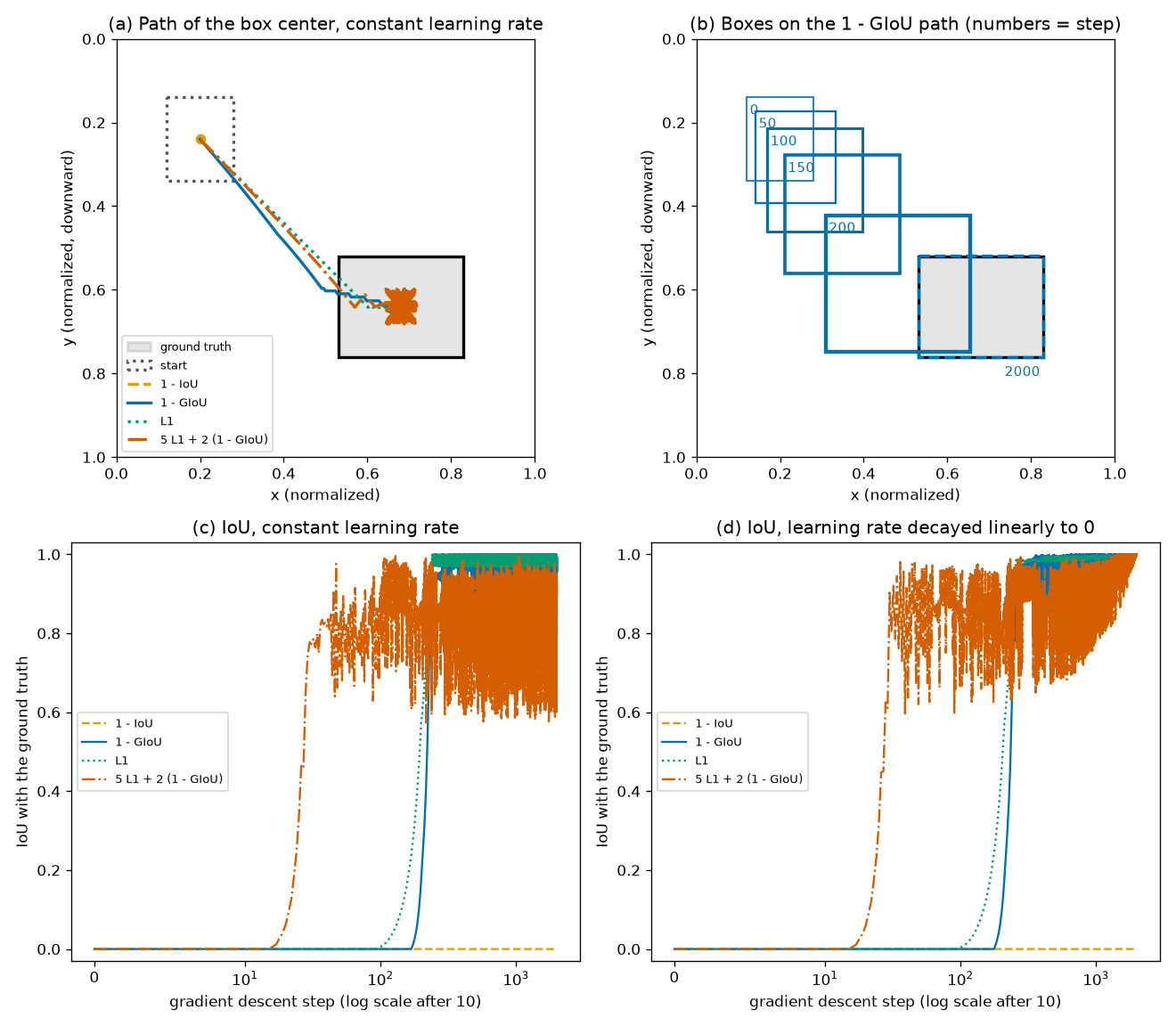
Let's read the results loss by loss, exactly as they are.
- \(1 - \operatorname{IoU}\): it did not move a single step. After 2,000 steps, the box is still the starting box \((0.200, 0.240, 0.160, 0.200)\) and IoU is 0. The gradient is exactly 0, so the result is the same no matter how many steps are run. It is the orange dotted line stuck to the bottom of Figure 2-7 (c), exactly as the derivation and the plain in Figure 2-6 predicted.
- \(1 - \operatorname{GIoU}\): it arrives, but by an unusual route. It reached IoU 0.5 at step 221 and 0.9 at step 244. But (b) shows the box growing steadily as it moves toward the target. The largest area along the way is 0.1150, about 1.6 times the target area of 0.0720 and about 3.6 times the starting area (\(0.16 \times 0.20 = 0.032\)). This is the \(\hat{w}\) gradient component seen earlier at work, that is, the property that while the boxes do not overlap, enlarging the box also reduces the loss. Only after reaching the target does the box shrink again. Also, for the first 169 steps it approaches with IoU stuck at 0 (no progress at all as far as IoU is concerned), and once overlap begins it climbs to 0.9 within 75 steps, because the gradient grows as the box gets closer (right side of Figure 2-5).
- L1: it moves at a constant speed. Overlap begins at step 90, IoU reaches 0.5 at step 195 and 0.9 at step 234. The gradient magnitude is always 1 per component, so each of the four numbers moves exactly 0.002 toward the target per step. \(\hat{c}_x\) has 0.48 to go, which takes 240 steps, and \(\hat{c}_y\) has 0.40, which takes 200 steps. So the green dotted line in (a) is not a straight line toward the target: it runs along a 45° diagonal and then turns horizontal once \(\hat{c}_y\) arrives first. The box area never exceeded the target area along the way.
- \(5 \cdot \text{L1} + 2 \cdot (1 - \operatorname{GIoU})\): it arrives fastest but oscillates the most. IoU reaches 0.5 at step 28 and 0.9 at step 45. But this speed is not the effect of combining the two losses. Multiplying the loss by 5 also multiplies the gradient by 5, which is exactly the same as multiplying the learning rate by 5. The price is larger oscillation around the target: over the last 200 steps, IoU swings between 0.5881 and 0.9775, ending at 0.7986. The red clump visible in the middle of the target in (a) is that oscillation.
Why does the oscillation happen? The L1 gradient has magnitude 1 even right next to the target. So even with only 0.0005 left to go, the box moves 0.002, overshoots to the other side, and comes back on the next step. That is why, with L1 alone, IoU jitters between 0.9704 and 1.0000 in the final stretch. With the coefficient 5, each step becomes 0.01 and the jitter grows fivefold. The GIoU loss is also sharp at the target (in the left panel of Figure 2-5, \(d = 0\) was a kinked corner). So even with \(1 - \operatorname{GIoU}\) alone, IoU oscillates between 0.8167 and 0.9941 in the final stretch.
The fix is to decrease the learning rate over time. The bottom four lines of the output and Figure 2-7 (d) show the results of running the same 2,000 steps while decreasing the learning rate linearly from 0.002 to 0. Except for \(1 - \operatorname{IoU}\), stuck on the non-overlapping plain, the other three all settled onto the target with IoU 0.9999–1.0000. Real detector training uses an optimizer that adapts gradient magnitudes on its own (AdamW, Chapter 4) together with a small learning rate, and it adjusts the neural network's weights rather than the box numbers directly, so the situation is somewhat different. Still, the property that the L1 gradient does not shrink remains.
- What this experiment showed
- The IoU loss cannot move non-overlapping boxes. The GIoU loss moves them but is slow from afar and inflates the box. L1 pulls the coordinates at a constant speed regardless of distance, but because its gradient never shrinks, it settles only when the learning rate is reduced.
- What this experiment did not show
- In this single-box experiment, there was no evidence that combining the two losses works better than using either alone. The combined loss was faster only because of its coefficients. The benefit of using both shows up in real detection training, with countless objects of varying sizes, and the evidence for it is presented in the next section through a table from the DETR paper.
Looking at the shapes world
Finally, let's look at IoU and GIoU on a shapes-world image. Pick one image with four objects and add noise to the four numbers of each ground-truth box. The direction of the jitter is fixed, and only its strength \(\sigma\) ("sigma") is increased: 0.01, 0.03, 0.06, and 0.10. \(\sigma\) is relative to the image side, so on a 96-pixel image it corresponds to about 1, 3, 6, and 10 pixels.
def jitter_example(seed: int):
    """도형 세상 그림의 정답 박스를 여러 세기로 흐트러뜨리고 IoU · GIoU 를 잰다.

    같은 방향의 흐트러짐(표준 정규 난수 한 벌)에 세기 σ 만 곱해, 같은 픽셀 오차가 큰 박스와 작은 박스에 주는 영향을 본다.
    """
    from rf_shapes import CLASS_NAMES_KO, ShapesDataset

    dataset = ShapesDataset(16, size=96, seed=0)
    index = next(i for i, t in enumerate(dataset.targets) if len(t["labels"]) == 4)  # 객체가 4개인 첫 그림
    image, target = dataset[index]
    boxes = target["boxes"]  # (4, 4) 정규화 (cx, cy, w, h)
    generator = torch.Generator().manual_seed(seed)
    direction = torch.randn(boxes.shape, generator=generator)  # 흐트러뜨릴 방향 (4, 4)
    levels = (0.01, 0.03, 0.06, 0.10)
    print(f"[9] 도형 세상 그림 {index}번의 정답 박스를 흐트러뜨리기 (σ 는 그림 한 변에 대한 비율, 96 픽셀이면 σ × 96 픽셀)")
    print("  객체      너비 × 높이(픽셀)  " + "  ".join(f"σ={s:.2f} IoU / GIoU " for s in levels))
    rows = []
    for sigma in levels:
        noisy = boxes + sigma * direction
        noisy[:, 2:].clamp_(min=0.02)
        iou = paired_box_iou(box_cxcywh_to_xyxy(noisy), box_cxcywh_to_xyxy(boxes))
        giou = paired_generalized_box_iou(box_cxcywh_to_xyxy(noisy), box_cxcywh_to_xyxy(boxes))
        rows.append((sigma, noisy, iou, giou))
    for k in range(len(boxes)):
        cells = "  ".join(f"     {iou[k].item():.3f} / {giou[k].item():6.3f}" for _, _, iou, giou in rows)
        print(f"  {CLASS_NAMES_KO[int(target['labels'][k])]:<5}    {boxes[k, 2].item() * 96:5.1f} × {boxes[k, 3].item() * 96:5.1f}    {cells}")
    return image, target, rows
[9] 도형 세상 그림 0번의 정답 박스를 흐트러뜨리기 (σ 는 그림 한 변에 대한 비율, 96 픽셀이면 σ × 96 픽셀)
  객체      너비 × 높이(픽셀)  σ=0.01 IoU / GIoU   σ=0.03 IoU / GIoU   σ=0.06 IoU / GIoU   σ=0.10 IoU / GIoU
  사각형       20.7 ×  14.5         0.777 /  0.770       0.470 /  0.418       0.203 /  0.043       0.025 / -0.303
  삼각형       29.7 ×  33.0         0.889 /  0.888       0.698 /  0.687       0.469 /  0.425       0.240 /  0.128
  삼각형       36.6 ×  28.0         0.903 /  0.902       0.739 /  0.734       0.551 /  0.533       0.370 /  0.329
  원         23.8 ×  23.8         0.867 /  0.865       0.659 /  0.642       0.439 /  0.384       0.242 /  0.124
그림 5장을 figures/ch02-*.png 로 저장. 걸린 시간 8.3초
- Figure: Figure 2-8. Ground-truth boxes and jittered boxes in the shapes world — four images showing the ground-truth boxes (solid green) and the jittered boxes (dashed orange), with the IoU written above and the GIoU below each object. From the left, the noise is about 1, 3, 6, and 10 pixels.
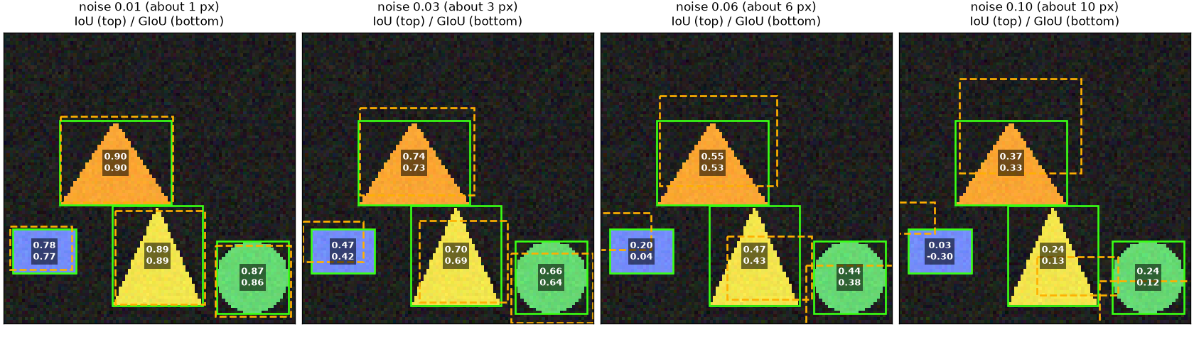
- Noise of about 1 pixel (leftmost): to the eye the two boxes almost coincide, yet IoU is 0.777–0.903. This confirms once again how strict a criterion IoU 0.9 is.
- Small objects break down first. The smallest rectangle (20.7 × 14.5 pixels) already falls below 0.5 at 3 pixels of noise, with IoU 0.470. With the same noise, the largest triangle (36.6 × 28.0 pixels) still has 0.739. (The noise direction differs from object to object, so this is not a rigorous comparison, but it matches the trend in the earlier table.)
- The gap between IoU and GIoU widens as misalignment grows. At noise 0.01 the two are nearly equal (0.777 and 0.770). At noise 0.10, the rectangle has IoU 0.025 and GIoU −0.303. IoU only says "barely overlapping," while GIoU goes further and says "and on top of that, there is this much empty space."
The DETR-family box loss
Putting everything so far into one line gives the box loss used by DETR and its descendants (Deformable DETR, LW-DETR, RF-DETR). For one pair of a matched predicted box \(\hat{b}\) and ground-truth box \(b\),
\(\mathcal{L}_{\text{box}}(b, \hat{b}) = \lambda_{\text{L1}}\,\|b - \hat{b}\|_1 + \lambda_{\operatorname{GIoU}}\,\big(1 - \operatorname{GIoU}(b, \hat{b})\big), \qquad \lambda_{\text{L1}} = 5, \quad \lambda_{\operatorname{GIoU}} = 2\)
\(\lambda\) ("lambda") is a coefficient (hyperparameter) that sets the mixing ratio of the two losses. The values 5 and 2 come from the DETR paper, and the LW-DETR paper and the public RF-DETR code (bbox_loss_coef=5.0, giou_loss_coef=2.0) use the same values. L1 is computed in the normalized center format \((c_x, c_y, w, h)\), and GIoU is computed after converting to the corner format. detr_box_loss in the code implements this formula.
Why the two are used together can be explained by what we have seen in this chapter.
| L1 | \(1 - \operatorname{GIoU}\) | |
| What it measures | The difference in each of the four numbers | Overlap and the fraction of empty space |
| With respect to box size | Size-blind: the same value for the same error on large and small boxes | Scale invariant: the same value for the same relative misalignment |
| When far apart | Gradient magnitude is always 1; pulls steadily | Gradient survives but weakens, and the box gets inflated |
| Near the target | Gradient does not shrink | The smaller the box, the larger the gradient |
| Relation to the scoring yardstick (IoU) | Indirect | Direct (IoU minus only the empty-space penalty) |
L1 pulls the coordinates directly, regardless of distance, while GIoU raises the overlap as measured by the scoring yardstick, regardless of size. Each fills in where the other falls short. The DETR paper explains that it linearly combines the L1 loss with the scale-invariant GIoU loss to mitigate the L1 loss's dependence on box size, and it reports an ablation that removes the loss terms one at a time (Table 4).
| Box loss (DETR paper Table 4, COCO) | AP | AP50 |
| L1 only | 35.8 | 57.3 |
| GIoU only | 39.9 | 61.6 |
| L1 + GIoU | 40.6 | 61.6 |
AP is the overall score of a detector, covered in Chapter 3 (higher is better). These numbers are not from our mini experiment; they are what the paper reported on the COCO dataset. The GIoU loss alone delivers most of the performance, L1 alone falls well short, and combining the two gives the best result.
The pieces from this chapter reappear later as follows.
- Chapter 3: the criterion for counting a prediction as a hit on a ground truth is an IoU threshold. NMS also uses IoU to filter out overlapping predictions.
- Chapter 7: the L1 distance and \(-\operatorname{GIoU}\) enter the matching cost, which decides which prediction is paired with which ground truth, as all pairs; once the pairs are decided, the \(\mathcal{L}_{\text{box}}\) above enters the loss as paired values.
- Chapter 9–Chapter 11: paired IoU is used in the IoU-aware loss, which sets the target value of the classification score to the IoU between the predicted box and the ground-truth box.
Note: variants that followed GIoU. GIoU has blind spots too. In the bottom row of Figure 2-3, the two "same center, different size" cases have a GIoU of 0.50, the same as their IoU. When one box contains the other entirely, the enclosing box \(C\) is the larger box itself, so there is no empty space and GIoU adds nothing to IoU. We also saw in this chapter's experiments that the gradient weakens from afar. Variants that address these issues include DIoU and CIoU (Zheng et al., "Distance-IoU Loss: Faster and Better Learning for Bounding Box Regression," AAAI 2020). According to the paper's abstract, DIoU adds the normalized distance between the predicted box and the target box to the loss, and CIoU takes three geometric factors into account together: overlap area, central point distance, and aspect ratio. Since the DETR family uses GIoU, this tutorial only mentions them by name and does not cover their formulas.
Summary
- A box is four numbers. The corner format \((x_0, y_0, x_1, y_1)\) is used for computing area and overlap; the center format \((c_x, c_y, w, h)\) is used for prediction and the L1 distance. The origin is at the top left, and \(y\) increases downward.
- Boxes in this tutorial use normalized coordinates from 0 to 1, which stay the same when the resolution changes. The center of pixel \(j\) is \((j + 0.5)/\text{size}\).
- The intersection rectangle is "max for the top left, min for the bottom right," clamped to 0 if there is no overlap. The union is \(|A| + |B| - |A \cap B|\).
- \(\operatorname{IoU} = |A \cap B| / |A \cup B|\): between 0 and 1, symmetric, 1 only when the boxes are identical, and scale invariant. An offset of just 1/3 of the width brings it to 0.5, and the smaller the box, the more it drops for the same pixel error.
- All-pairs computation produces an
(N, M)table by broadcasting(N, 1, 2)against(1, M, 2); paired computation produces(K,). The former is for matching, the latter for losses. - The L1 loss pulls with a constant gradient everywhere but does not know the box size. The IoU loss is scale invariant, but its gradient is 0 when the boxes do not overlap.
- \(\operatorname{GIoU} = \operatorname{IoU} - (|C| - |A \cup B|)/|C|\). \(-1 \lt \operatorname{GIoU} \le \operatorname{IoU} \le 1\), and even without overlap it decreases with distance, so the gradient survives.
- The DETR-family box loss is \(5 \cdot \text{L1} + 2 \cdot (1 - \operatorname{GIoU})\).
We can now say in numbers how similar two boxes are. But a detector outputs dozens of boxes per image, and they include hits, wild misses, and duplicates pointing at the same object. Giving this whole pile of predictions a single score requires one more layer on top of IoU. The next chapter splits predictions into hits and misses with an IoU threshold, and computes precision, recall, and the detector's report card, AP and mAP, by hand.
Review questions
- 1. Converting formats — Convert the box with normalized center format \((c_x, c_y, w, h) = (0.5, 0.4, 0.2, 0.6)\) to the corner format, and find its pixel coordinates in a 96×96 image. Horizontally, which pixels does this box cover, from which to which (using the pixel-center convention)?
- \((0.5 - 0.1,\ 0.4 - 0.3,\ 0.5 + 0.1,\ 0.4 + 0.3) = (0.4, 0.1, 0.6, 0.7)\). Multiplying by 96 gives \((38.4,\ 9.6,\ 57.6,\ 67.2)\). Horizontally, it covers the pixels whose center \(j + 0.5\) is at least \(38.4\) and at most \(57.6\): from \(j = 38\) (center 38.5) to \(j = 57\) (center 57.5), 20 pixels in all.
- 2. IoU and GIoU by hand — For \(A = (0, 0, 4, 4)\) and \(B = (2, 2, 6, 6)\) (corner format), find the intersection, the union, IoU, the enclosing box \(C\), and GIoU.
- Both areas are 16. Intersection: horizontally \(\min(4, 6) - \max(0, 2) = 2\), vertically also 2, so the area is 4. Union \(16 + 16 - 4 = 28\). \(\operatorname{IoU} = 4/28 = 1/7 \approx 0.1429\). \(C = (0, 0, 6, 6)\), with area 36 and empty space \(36 - 28 = 8\). \(\operatorname{GIoU} = 1/7 - 8/36 \approx 0.1429 - 0.2222 = -0.0794\). GIoU is negative even though the boxes overlap.
- 3. Separated boxes — Find the IoU and GIoU of \(A = (0, 0, 2, 2)\) and \(B = (4, 0, 6, 2)\). What value results if the horizontal overlap is not clamped to 0? Also verify GIoU with the formula \(\frac{w - d}{w + d}\).
- Horizontal overlap \(\min(2, 6) - \max(0, 4) = -2\) → clamped to 0, the intersection is 0 and IoU is 0. Without clamping, it becomes a negative area of \((-2) \times 2 = -4\), the union grows to \(4 + 4 + 4 = 12\), and IoU becomes the nonsensical value \(-1/3\). Computed correctly, the union is 8, \(C = (0, 0, 6, 2)\) has area 12, and \(\operatorname{GIoU} = 0 - (12 - 8)/12 = -0.3333\). By the formula, \(w = 2\) and \(d = 4\), so \((2 - 4)/(2 + 4) = -1/3\). They agree.
- 4. How accurate does it need to be? — For a box 20 pixels wide, the size is predicted exactly but the horizontal position is off. How many pixels of error at most give an IoU of 0.9 or higher? An IoU of 0.5? What if the width is 100 pixels?
- \(d = w\,\frac{1 - \operatorname{IoU}}{1 + \operatorname{IoU}}\). IoU 0.9: \(d = 20/19 \approx 1.05\) pixels. IoU 0.5: \(d = 20/3 \approx 6.67\) pixels. With a width of 100, the values are \(100/19 \approx 5.26\) and \(100/3 \approx 33.3\) pixels, respectively. The allowed error is proportional to the width. For small boxes, it comes down to a single pixel.
- 5. Tracing shapes — When
boxes1has shape(300, 4)andboxes2has shape(7, 4), write down the shapes ofleft_top,wh,inter, andunioninsidebox_iou, in order. What happens if you callpaired_box_iou(boxes1, boxes2)? -
left_top:(300, 1, 2)against(1, 7, 2)→(300, 7, 2).wh:(300, 7, 2).inter:(300, 7).union:(300, 1) + (1, 7) − (300, 7)→(300, 7). The paired function tries to compare(300, 2)and(7, 2)directly; the leading axis lengths, 300 and 7, are neither equal nor 1, so a broadcasting error occurs. The paired function must be given the same number of boxes, already paired up. - 6. Computing the box loss — Find the box loss \(5 \cdot \text{L1} + 2 \cdot (1 - \operatorname{GIoU})\) for the ground truth \(b = (0.5, 0.5, 0.2, 0.2)\) and the prediction \(\hat{b} = (0.6, 0.5, 0.2, 0.2)\) (normalized center format). What would the loss be if both the width and height of the boxes were 0.4 (with the centers unchanged)? Which term accounts for the difference between the two results?
- L1 is \(|0.5 - 0.6| = 0.1\) (the other components are equal). The boxes have the same size and are shifted only horizontally by \(d = 0.1\), so \(\operatorname{GIoU} = \operatorname{IoU} = \frac{w - d}{w + d} = \frac{0.1}{0.3} = 0.3333\). Loss \(= 5 \times 0.1 + 2 \times (1 - 0.3333) = 0.5 + 1.3333 = 1.8333\).
- With a width of 0.4, L1 is still 0.1, \(\operatorname{GIoU} = \frac{0.4 - 0.1}{0.4 + 0.1} = 0.6\), and the loss \(= 0.5 + 2 \times 0.4 = 1.3\). The L1 term is identical in both cases (it does not know the size), and the entire difference of 0.5333 comes from the GIoU term. It is the GIoU term that penalizes the same 0.1 error more heavily on the smaller box.
- Try it yourself
- Change the starting box in
descent_experimentso that it slightly overlaps the target (e.g.,[0.50, 0.50, 0.16, 0.20]) and run it. This time \(1 - \operatorname{IoU}\) should move as well. Also lowerlr=0.002inmainto 0.0004, observe how the convergence steps and the final-stretch oscillation of5 L1 + 2 (1 - GIoU)change, and compare them with the original result for L1 alone.
See also
- RF-DETR:Tutorial
- RF-DETR
- Object detection
- Bounding box
- Intersection over Union
- Gradient descent
- PyTorch